Abstract
Modern neural networks addressing dense Non-Rigid Structure from Motion (NRSFM) dilemmas often grapple with intricate a priori constraints, deterring scalability, or overlook the imperative of consistent application of a priori knowledge throughout the entire input sequence. In this paper, an innovative neural network architecture is introduced. Initially, the complete 2D sequence image undergoes embedding into a low-dimensional space. Subsequently, multiple self-attention layers are employed to extract inter-frame features, with the objective of deriving a more continuous and temporally smooth low-dimensional structure closely resembling real data’s intrinsic structure. Moreover, it has been demonstrated by others that gradient descent during the training of multilayer linear networks yields minimum rank solutions, implicitly providing regularization that is equally applicable to this task. Benefiting from the excellence of the proposed network architecture, no additional a priori knowledge is mandated, barring the constraint of temporal smoothness. Extensive experimentation confirms the method’s exceptional performance in addressing dense NRSFM challenges, outperforming recent results across various dense benchmark datasets.
1. Introduction
Non-rigid Structure from Motion (NRSFM) is a significant research direction in computer vision that aims to estimate the 3D shape of non-rigid objects from videos. However, recovering 3D structure from 2D images poses a challenging inverse problem. A video can be considered as a collection of multi-frame images, and to achieve reconstruction, motion and deformation information between frames, along with prior assumptions, can be utilized.
Depending on the characteristics of the reconstructed object, the NRSFM problem can be divided into NRSFM with sparse feature points and NRSFM with dense feature points. Dense feature points are more numerous and accurate in rendering the surface of non-rigid objects compared to sparse feature points. Despite significant results achieved by existing sparse NRSFM methods, their performance in extending to the case of dense feature points remains unsatisfactory [1,2,3,4,5]. Recent progress has been made in dedicated algorithms for dense NRSFM problems [6,7,8,9].
The rise of deep learning has led to an increased focus on solving the challenges in NRSFM using neural networks, resulting in significant advancements. To address the challenge of dense feature points, Sidhu et al. [6] proposed the learnable neural network (N-NRSFM), which employs an automatic decoder model to assign a latent variable to each 3D shape and imposes constraints in the latent space to ensure similar 3D shapes have similar latent variables. This approach enhances robustness, scalability, and achieves lower 3D reconstruction errors in various scenarios. However, the method relies on the Tomas–Kanade decomposition [10] for solving the 3D mean shape and is sensitive to 2D trajectories with large errors. Inspired by Deng et al.’s study [11], where each frame does not exist independently but rather as part of a sequence, and the prior constraint should apply to the entire sequence rather than a single frame, the N-NRSFM method overlooks this point. Thus, it is important to revisit the NRSFM problem from this perspective to “translate” the input 2D image sequence into a 3D sequence structure.
Recently, the Transformer architecture has been widely employed in Sequence-to-Sequence models, utilizing a self-attention mechanism to extract information between sequences, making it particularly suitable for solving NRSFM tasks. Additionally, Jing L et al. [12] demonstrated that optimizing multiple linear neural network layers through an iterative gradient-based optimization approach can yield low-rank output results. They conducted experiments on an autoencoder model to support this finding, which is also applicable to implicit regularization in NRSFM. Another intuitive idea is that neighboring frames should be adjacent in a low-dimensional space to ensure smoothness of the 3D structure over time.
Based on the aforementioned ideas, this paper proposes a novel neural network structure. Firstly, the entire original 2D sequence image is embedded into a low-dimensional space. Then, features between each frame are extracted using multiple self-attention layers, aiming to obtain a potential low-dimensional structure that is more continuous and smooth over time, closely resembling the intrinsic structure of the real data. Furthermore, in lieu of incorporating additional neural network modules for optimizing the rotation matrix, Orthogonal Procrustes (OnP) is employed to compute the required rotation matrix. Due to the problem’s specificity, the method is trained entirely in an unsupervised manner, independent of any reliance on ground truth values. Conclusively, the experimental outcomes on dense datasets underscore the excellence of the presented neural network framework.
The main contributions of this work can be summarized as follows:
- A novel neural network structure is introduced for addressing dense NRSFM problems. The method processes the entire 2D sequence as input and transforms it into a structured 3D sequence. No additional a priori constraints are employed, except for the regulation of deformation between neighboring frames to improve temporal smoothness.
- Multiple linear layers devoid of activation functions and bias values are introduced for the implicit regularization of latent variables within the low-dimensional space. Subsequent experimental results validate this approach. Furthermore, the extraction of features between frames within the low-dimensional space is achieved through the utilization of multilayer self-attention layers, fostering the acquisition of a more meaningful and smoother latent space.
- The proposed method attains state-of-the-art performance on a dense benchmark dataset, underscoring the strengths of this approach in managing sequential data.
2. Related Work
2.1. Classical NRSFM Approaches
In the field of computer vision, considerable progress has been made over the past few decades in addressing the challenging problem of recovering 3D structures from 2D images. Several influential research directions have emerged, warranting attention in this context. One such direction is the shape space model, which is based on the low-rank assumption [13]. This model has been widely adopted to characterize the deformation of non-rigid objects, allowing for their recovery and analysis by constraining shape changes to a low-dimensional subspace. Another noteworthy approach is the trajectory space model [14], which describes the motion trajectory of non-rigid objects and infers three-dimensional structural information from it.
The probabilistic principal component analysis model (PPCA) [15] has also found important applications in computer vision. It employs probabilistic models to describe the data generation process and employs maximum likelihood estimation to infer the latent variables and model parameters. PPCA is advantageous in modeling non-rigid object deformation and motion.
The manifold hypothesis [16,17,18] constitutes another significant research direction, positing that object deformation and motion can be represented by low-dimensional manifolds. This idea has inspired subsequent methods such as the Grassmannian manifold method (GM) [9]. Moreover, the jump manifold method (JM) [19] serves as an extension of GM, considering the relationship between local surface deformation and point domains and utilizing high- and low-dimensional Grassmannian manifolds for modeling and reconstructing non-rigid object deformation.
In addition to the aforementioned approaches, the block matrix method (BMM) introduced by Dai [20] transforms the low-rank constraint into a semi-positive definite programming and kernel parametric minimization problem, providing a novel idea for non-rigid structure recovery. The SMSR method by Ansari [21] updates the input measurement matrix by applying trajectory smoothing constraints and employs the alternating direction multiplier method (ADMM) to optimize the objective function.
Furthermore, Lee et al. proposed the classical Expectation Maximization–Procrustean Normal Distribution (EM-PND) model [22] based on the generalized Procrustes analysis (GPA) [23]. This model does not require additional constraints or priors and can be applied to recover non-rigid objects at different time points. However, in practical scenarios, objects typically exhibit temporal variations, and enforcing smoothness becomes a crucial constraint for non-rigid 3D structure recovery. To address this, Lee et al. further proposed the Procrustean Markov Process (PMP) algorithm [24], which combines the PND assumption with a first-order Markov model to enable smooth recovery and modeling of non-rigid objects.
2.2. Neural-Network-Based Solutions for NRSFM
In recent years, the application of neural networks to solve the NRSFM problem has gained popularity among researchers [25,26,27]. Cha et al. [28] utilized a low-rank loss as the learning objective to constrain the shape output of their 2D–3D reconstruction networks. Novotny [27] proposed the C3DPO model, which employed low-rank factorization and consisted of two branches for viewpoint and shape prediction. The model achieved decoupling and self-consistency of the branches by employing auxiliary neural networks to normalize the 3D shape of randomly rotated projections. On the other hand, Park et al. [29] achieved significant results by introducing a loss function that automatically determined the appropriate rotation for shape alignment, despite the relative simplicity of their underlying network structure.
Regarding the low-rank constraint, the shape basis (i.e., the rank parameter) plays a crucial role in reconstruction error. In previous NRSFM algorithms, the weights for low-rank, subspace, or compressed priors (e.g., rank or sparsity) often required tedious cross-validation for selection. However, Chen Kong et al. [25] proposed a deeply interpretable NRSFM network, known as Deep Neural Networks (DNNs), based on classical sparse dictionary learning and deep neural networks. This method eliminated the need for tedious cross-validation by simultaneously learning the prior weights and other parameters. They further extended their approach to handle occlusion and loss of feature points [30]. Wang et al. [31] advanced this approach by proposing the Deep-NRSFM++ model, which accounted for more realistic situations, including perspective projection cameras and critical occlusion. Ma et al. [32] built upon this approach by incorporating multi-view information and designing a simple yet effective loss function to ensure decomposition consistency. Subsequently, Zeng et al. [33] proposed a new residual recurrent network and introduced the Minimal Singular Value Ratio (MSR) as a metric for measuring shape rigidity between two frames. Based on this metric, they employed two novel pairwise loss functions to constrain the feature representation of 3D shapes, achieving advanced shape recovery accuracy in large-scale human motion and classified object reconstruction.
In contrast to classical NRSFM priors, some researchers have explored constraints provided by deep learning itself. Generative adversarial networks (GANs) have been utilized to predict lost depth information by enhancing 2D reprojection realism from different viewpoints [34,35,36,37]. However, due to the requirements of GAN learning, these methods are only applicable to large-scale datasets. Deng et al. [11] introduced the Sequence-to-Sequence (Sequence-to-Sequence) model to the NRSFM task, proposing the use of a multi-headed attention mechanism instead of a self-representation layer to impose priori subspace concatenation structures. Sidhu et al. [6] employed unsupervised neural networks for 3D reconstruction in dense NRSFM and achieved excellent results using automatic decoder deformation models and latent space constraints. Wang et al. [1] proposed the PAUL model, which argued that aligned 3D shapes could be compressed by depth under complete autoencoders. They further proposed the neural trajectory prior (NTP) for motion regularization [38]. The method can also be applied to other 3D computer vision tasks, including scene stream integration and dense NRSFM. Similar to N-NRSFM and PAUL, they introduced a bottleneck layer in the model to compress the generated trajectories into a low-dimensional space.
Despite the remarkable advancements in neural-network-based NRSfM in recent years, the emphasis has primarily been on the 3D reconstruction of sparse objects. The field of neural-network-based dense NRSfM is still in its nascent stage, leaving ample room for further exploration and development.
3. Proposed Method
3.1. Problem Background
Before introducing the approach, a brief overview of the classical NRSFM problem is provided. In cases where the object is considered rigid, it does not deform during motion, maintaining a constant relative distance between key points. In the structure from motion, a relative rigid transformation, often referred to as rotation, is required between the camera and the reconstructed object. This transformation can involve scenarios where the camera remains fixed while the object undergoes a rigid transformation, or vice versa. Alternatively, both the camera and the object may undergo a relative rigid transformation. Typically, the assumption is that the object remains stationary while the camera undergoes a rigid transformation.
The input to the NRSFM problem is a 2D trajectory matrix , consisting of P 3D points projected onto F frames. Each frame image , denoted as the i-th frame, contains P 2D coordinates. To simplify the problem, it is assumed that orthogonal camera projection is used, meaning that the projection of 3D points to 2D coordinates only considers the components while ignoring the depth z, i.e., . Following the camera projection model, the following equations are derived:
Here, represents the P 3D coordinate points of the rigid object. denotes the rotational component of the rigid body transformation performed per frame, satisfying under the condition of orthogonal projection. Additionally, represents the translational component of the rigid body transformation performed per frame. By assuming that the origin of the world coordinate system is positioned at the object’s center of gravity, the problem is further simplified through subtraction of the row-wise average of the W matrix from each row, effectively eliminating . This leads to the following equation:
In Equation (2), the measurement matrix is obtained by subtracting the average value of each row of the W matrix. The aforementioned discussion focuses on the case of reconstructing a rigid object. However, in the case of a non-rigid object, is no longer fixed in each frame due to deformation, leading to potential changes in the relative distance between key points. As a consequence, extends to . This modification leads to an altered projection equation:
Here, . With reference to Equation (3), the aim is to recover the unknown 3D shape S from the known measurement matrix .
3.2. Method Overview
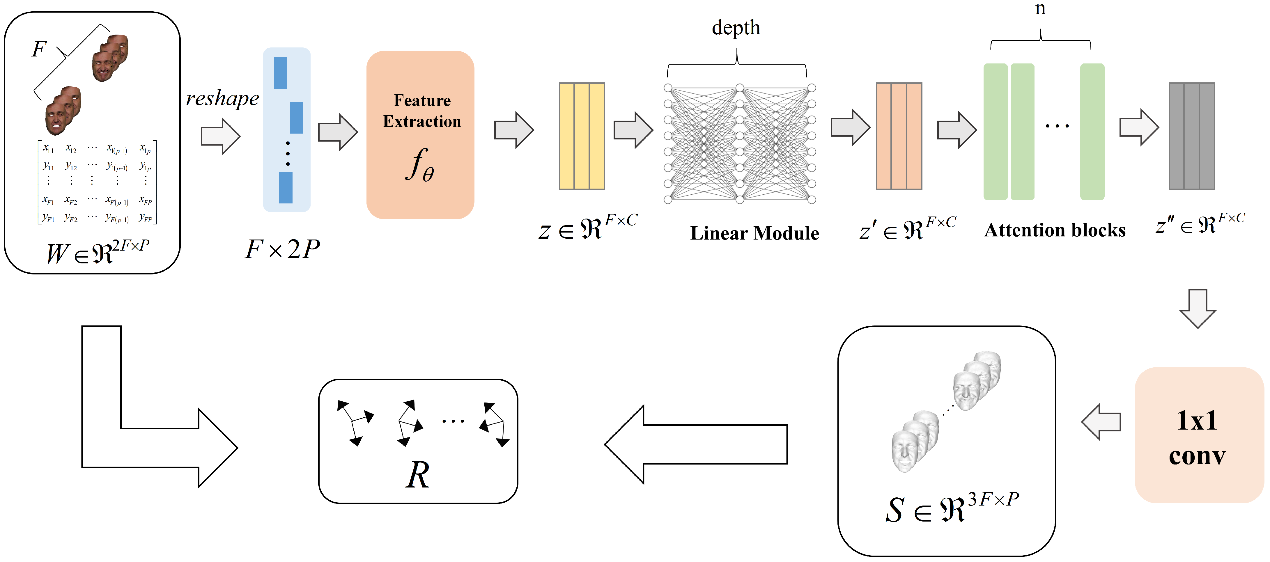
The architecture of the proposed model is illustrated in Figure 1. Initially, the entire measurement matrix serves as input and is transformed into for compatibility with the model. Subsequently, the feature extraction module downscales the input, resulting in the feature representation . To incorporate implicit regularization, a multilayer linear layer module is employed, without activation functions or bias values, to further process the feature representation and derive a lower-rank feature representation .
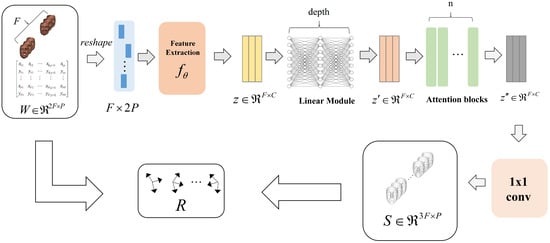
Figure 1.
An overview of the devised neural network architecture, which comprises a feature extraction module, a multilayer linear module, and multiple self-attention modules. The network operates by ingesting the complete measurement matrix as input and subsequently transforming it into a 3D structure. During the training phase, the network is guided by a reprojection loss and an additional temporal constraint.
Recognizing the inherent continuity in the low-dimensional space between adjacent frames, the aforementioned feature representation is fed as a sequential input to a multilayer self-attention module. This allows for the capture of feature relationships between frames and the derivation of a potentially lower-dimensional structure characterized by increased temporal continuity and smoothness. To reduce the parameter count, a 1 × 1 convolution module is employed to decode the output of the self-attention module and map it to a real 3D structure S.
Finally, the rotational component R between the input measurement matrix and the 3D structure S is computed using a simplified OnP solver. Importantly, it should be noted that the entire reconstruction process relies solely on self-supervision and does not necessitate actual camera motion information or supervised training with non-rigid shapes. Consequently, the proposed model enables unsupervised non-rigid shape reconstruction.
3.3. Feature Extraction Module
The feature extraction module plays a crucial role in downscaling the input measurement matrix. Let the input measurement matrix be denoted as , and the output of the feature extraction module is represented as , which can be expressed as:
Network Input: Regarding the input of the network, the measurement matrix can be reshaped into a feature tensor , where F represents the number of frames and denotes the number of channels. After this transformation, the feature representation can be fed into the convolutional layer.
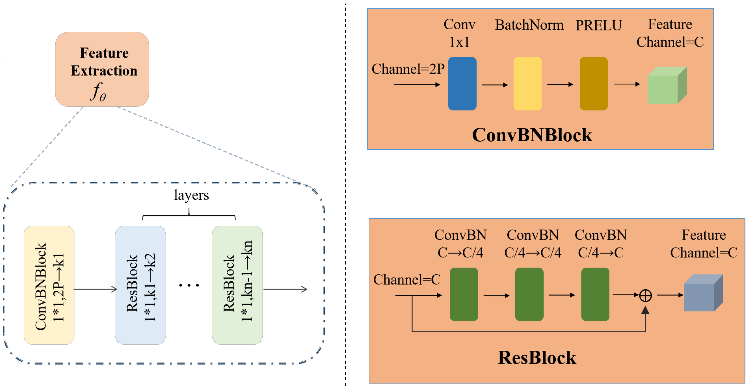
Network Structure: The structure of the network is illustrated in Figure 2 and comprises a ConvBNBlock module and layers of ResBlock modules. This design follows a classical architecture incorporating convolutional layers, batch normalization, and activation functions. By utilizing a 1 × 1 convolutional kernel, the network compresses the number of channels from to C. This design not only alters the input and output channel dimensions but also preserves the shape of the feature tensor while effectively reducing the number of parameters. The ResBlock is a network module based on residual learning, which mitigates the problem of degradation in neural networks and facilitates the design of deeper network structures. It takes a tensor with C channels as input and processes it through three ConvBNBlock modules to obtain a new feature representation. Finally, the input and output data are directly summed, enabling the injection of input information into subsequent layers of the network. This approach promotes better gradient propagation within the network, facilitating the learning of residual information between the input and output. As a result, it optimizes the model parameters and enhances network performance.
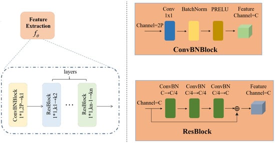
Figure 2.
The Feature Extraction Module involves incorporating a ConvBNBlock and a set of ResBlocks. In the context of this module, the notation signifies the transformation of a feature map with an input channel of c through a convolutional kernel of dimensions to generate an output with d channels.
3.4. Multilayer Linear Module
Based on a related study [12], it has been observed that the learning process of gradient descent in multilayer linear networks can lead to the occurrence of minimum rank solutions. Taking this finding into consideration, our approach incorporates multiple additional linear layers , with random initialization to explore a broader feature representation space. Typically, neural network architectures often rely on a single fully connected layer for feature aggregation. However, multiple fully connected layers, combined with activation functions and biases, are commonly used to achieve nonlinear transformations and enable more complex model representation capabilities. In contrast, our linear transformation module does not employ any nonlinear activation functions between the multilayer fully connected layers. This design choice is motivated by the fact that the linear transformation module aims, not for simple feature aggregation, but for implicit regularization through weight optimization. Through iterative optimization of these layers, our objective is to achieve implicit regularization, leading to improved output of the latent variables.
Following the linear transformation module, the learned latent variable typically exhibits a reduced numerical representation compared to the original latent variable , which has not undergone linear transformation. This reduction in numerical representation helps mitigate overfitting and enhances the model’s generalization ability. Consequently, our model can automatically learn representations with lower effective dimensions, effectively capturing essential features and structures within the data.
3.5. Multiple Self-Attention Module
In a previous study conducted by Deng et al. [11], an approach was introduced to regulate the subspace concatenation structure. This was achieved by incorporating a single layer of self-attention blocks, as opposed to self-expression layers. In contrast to this approach, the current study adopts a distinct strategy for managing latent variables within low-dimensional spaces. Multiple layers of self-attention blocks dedicated to feature extraction and encoding are employed. The integration of these self-attention blocks in a stacked manner facilitates the gradual extraction and encoding of feature information from the input sequence. Consequently, the model establishes a hierarchical structure, allowing for the progressive comprehension of semantic and contextual cues within the sequence. This, in turn, enhances the model’s ability to discern deformation and motion features in non-rigid objects, ultimately leading to a more profound and seamless representation in the potential space.
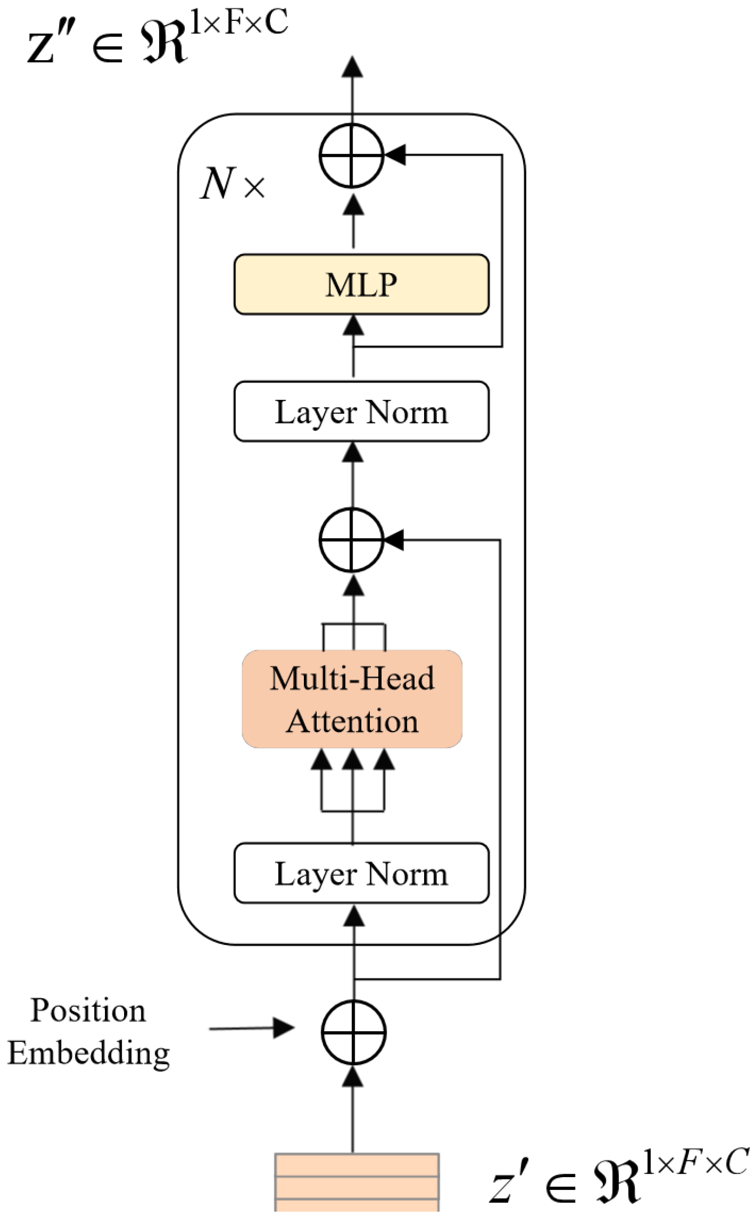
The self-attention block adopts a design similar to the Encoder module within the Transformer model, as depicted in Figure 3. It encompasses two primary modules: a multi-head self-attention mechanism and a multi-layer perceptron block. Preceding these modules, LayerNorm is applied for normalization, and subsequently, residual connections are integrated to ensure the coherent and consistent flow of information. The multi-head self-attention mechanism operates by concurrently modeling information across various locations within the representation subspace. It conducts scaled dot product attention in parallel and consolidates the results of h attention heads, as represented by the following expressions:
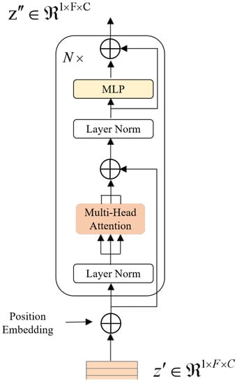
Figure 3.
The figure illustrates the structure of a single attention block within the neural network architecture. This block treats individual frames as sequence tokens, enabling the network to capture intricate relationships between frames. It operates as a fundamental building block for feature extraction and encoding, contributing to the network’s ability to progressively comprehend the semantic and contextual information within the input sequence.
In this context, “Attention” denotes scaled dot product attention. It involves the mapping of the input query matrix Q, key matrix K, and value matrix V to produce the output attention matrix. Here, . To maintain gradient stability, appropriate normalization is applied to the dot product attention. As a result, the output expression for scaled dot product attention can be defined as:
In the above expression, d denotes the dimension C of the input feature, N denotes the length F of the sequence, and Q, K, and V are computed from the input feature representation through linear transformations , i.e.,
Prior to handling the input feature , the encoding of its position is undertaken. A fixed position encoding method is utilized for this purpose:
Here, represents the position in the sequence, denotes the even dimension, and denotes the odd dimension (i.e., ). The input, embedded with position encoding, is then passed through N Encoder modules to obtain a new feature representation . Ultimately, this representation is decoded using a 1 × 1 convolution module to transform it into a tangible 3D structure S.
3.6. Rotation Estimation
The deformation of non-rigid body shapes can sometimes be mistaken as camera motion, potentially compromising the quality of the reconstruction. To tackle this issue, a straightforward and efficient method is introduced for recovering camera motion without requiring additional neural network modules. This problem is approached as a classical mathematical challenge referred to as the Orthogonal Procrustes problem (OnP problem), which is widely used in the estimation and matching of rotation matrices. The formulation is as follows:
To address this problem, the following steps are taken:
- Each frame, denoted as frame i, is initially transformed into a least squares problem. It is then solved to obtain .
- As the previous solution does not incorporate the orthogonality constraint of , a projection of onto an orthogonal matrix is performed utilizing the SVD decomposition method. This process is illustrated by . The outcome of this operation is represented as the rotation matrix .
It is worth highlighting that this basic OnP solver might not perform optimally when dealing with coplanar 3D points. Nevertheless, it is important to emphasize that coplanarity is a seldom-seen phenomenon in real dynamic scenes, and during experiments, coplanarity has not been encountered. Through the adoption of this simple yet efficient method, accurate camera motion recovery is achieved, leading to an enhancement in the overall reconstruction quality. This approach circumvents the requirement for intricate neural network architectures, ensuring model interpretability and computational efficiency.
3.7. Loss Function
To enable unsupervised training of the network, this paper introduces a differentiable energy function E. This function facilitates gradient backpropagation and can be efficiently implemented and solved within modern neural network frameworks.The form is as follows:
The loss function is designed to constrain the reprojection error of the matrix. It measures the agreement between the 2D projection of the 3D structure estimated by the neural network and the given 2D feature points. This is achieved by utilizing the rotation matrix obtained from the rotation estimation module. The loss function is expressed as:
The loss function captures the level of deformation between adjacent frames, promoting temporal smoothness and enhancing the continuity and stability of the reconstruction results. The expression of the loss function is as follows:
In the equation above, denotes the Huber loss, while the coefficients and are employed to regulate the relative influence of each loss function on the ultimate structural outcome. Notably, this method operates independently of any extra a priori constraints, apart from ensuring deformation control between neighboring frames to promote temporal consistency. This attribute significantly enhances the scalability of the approach. The formulated loss function effectively directs the network’s training procedure, enabling it to acquire more robust and precise 3D reconstruction results.
4. Experimental Evaluation
4.1. Experimental Details
4.1.1. Datasets and Evaluation Metrics
Datasets: The experimental evaluation covers three different dataset types to comprehensively assess the performance and robustness of the method. First, widely used dense datasets containing samples with ground truth 3D shapes were utilized. One of these datasets is the Actor Mocap dataset, which offers actual facial data and corresponding 3D structural information. Additionally, synthetic facial datasets known as Synthetic Faces were employed, a common choice for testing and comparing NRSfM algorithm performance. Furthermore, real Kinect camera sequence datasets were incorporated to provide a more realistic representation of data in real-world application scenarios.
Secondly, relatively sparse datasets with realistic 3D geometries but fewer sample points were included. These datasets comprise the Expressions dataset and the Pants dataset. Due to the data’s sparsity, tackling these datasets presents a challenge for the approach.
Finally, real video sequence datasets, closely resembling real-world situations, were incorporated. This diverse range of datasets enables a comprehensive evaluation of the method’s performance in various scenarios. The deliberate selection of these datasets ensures the method’s adaptability and practicality, enhancing the representativeness and comparability of the experimental results.
Evaluation metrics: The performance of the algorithm on a dataset with real 3D structure is evaluated using the Normalized Mean 3D Error metric. The calculation for this metric is as follows:
In the equation, represents the real 3D structure of the reconstructed object, while represents the predicted 3D structure after aligning to the final 3D structure. This error metric quantifies the difference in distance between the reconstructed result and the ground truth. A smaller error value indicates that the reconstructed result is closer to the ground truth, implying higher accuracy of the algorithm.
4.1.2. Implementation Details
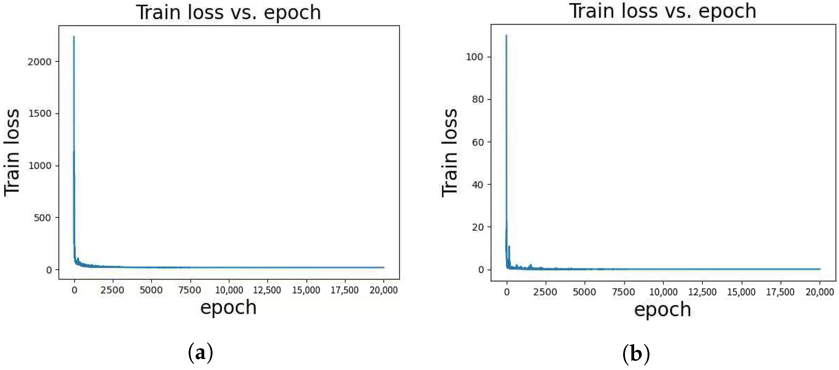
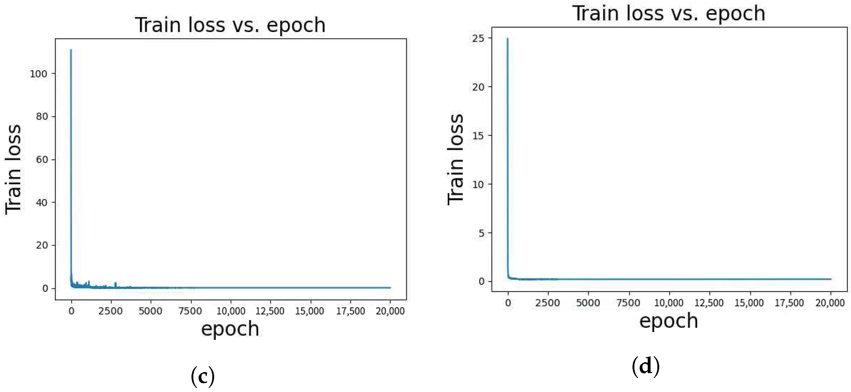
The implementation of the method is based on PyTorch version 1.12.0 with Python 3.8, CUDA 11.3, and cuDNN 8.3.2. The optimization process utilized the AdamW optimizer with an initial learning rate of 0.001 and amsgrad = True. During the training process, the number of layers in the feature extraction module remained fixed at 2, and the depth in the linear module was set to 8. A range of values for the number of N in the self-attention layer module was explored, spanning from 3 to 8. The dimension C of the potential feature representation was determined according to the specific characteristics of each dataset. In most cases, C was set to 256. However, for the Kinect dataset, C was set to 512, and for the Pants dataset, it was set to 128. To balance the loss terms, a weight coefficient of 40 was assigned to the loss term , while a weight coefficient of 1 was assigned to the loss term . The training process comprised 20,000 epochs to ensure convergence and model refinement. A learning rate scheduler was applied with a step size of 400 and a reduction factor of 0.95. Additionally, Figure 4 presents the training loss curves.
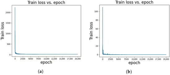
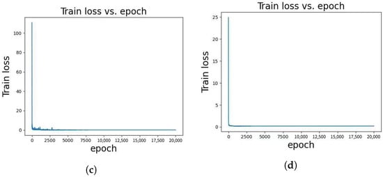
Figure 4.
(a) displays the training loss curve for the paper dataset, showing the evolution of the loss function during training on this dataset. (b) presents the training loss curve for the seq3 dataset, demonstrating how the loss changes as the model is trained on this dataset. (c) visualizes the training loss curve for the seq4 dataset, illustrating the loss dynamics during training on this dataset. Finally, (d) showcases the training loss curve for the Pants dataset, providing a view of the loss variation during training on this specific dataset.
4.2. Result Evaluation
4.2.1. Quantitative Results Evaluation
Synthetic Faces: The Synthetic Face dataset comprises two sequences, namely, syn3 and syn4, each featuring distinct camera trajectories. These sequences encompass 99 frames and include a total of 28,000 points. In the evaluation of the Synthetic Face dataset, a comparison was conducted between the 3D reconstruction framework employed and classical traditional methods such as VA [8] and CMDR [39]. Additionally, an assessment was made of newer traditional methods, including GM [9], JM [19], SMSR [21], PPTA [40], and EM-FEM [7], along with neural network methods like N-NRSfM [6], RONN [41], NTP [38], and DST-NRSFM [42]. Furthermore, comparisons were carried out with other relevant methods. The results of this comprehensive analysis for all the algorithms are presented in Table 1.

Table 1.
Comparison results for on the Synthetic Face sequences dataset reveal that the method proposed in this study exhibits the lowest error among the evaluated approaches, which include VA, CMDR, GM, JM, SMSR, PPTA, EM-FEM, N-NRSfM, RONN, NTP, and DST-NRSFM.
Actor Mocap: The Actor Motion Capture dataset comprises 100 frames, encompassing a total of 36,349 points. To gauge the effectiveness of the method on this dataset, a comparative evaluation was conducted against FML [43], SMSR [21], CMDR [39], RONN [41], N-NRSFM [6], and DST-NRSFM [42]. The outcomes, as shown in Table 2, reveal the superior performance and accuracy achieved by the proposed method. These findings underscore the efficacy of the approach, particularly when applied to the Actor Motion Capture dataset.
Table 2.
Comparing results on the Actor Mocap dataset, this study’s method is benchmarked against FML, SMSR, CMDR, RONN, N-NRSFM, and DST-NRSFM.
Expressions: The Expression dataset, characterized by its relative sparsity, consists of 384 frames and 997 points. In this study, a comparative analysis of this dataset was conducted involving several methods, namely, CSF2 [44], KSTA [17], GMLI [45], N-NRSFM [6], RONN [41], and DST-NRSFM [42]. The conclusive experimental results are presented in Table 3.
Table 3.
Assessing results on the Expressions dataset, this study’s method is compared against CSF2, KSTA, GMLI, N-NRSFM, RONN, and DST-NRSFM.
Pants: The Pants dataset exhibits a relatively sparse nature, comprising a total of 291 frames and 2859 points. In this study, an assessment of various methods on this dataset was conducted, encompassing KSTA [17], BMM [20], PPTA [40], and DST-NRSFM [42]. The outcomes of these comparative experiments are detailed in Table 4.Through a comprehensive analysis and comparison of the experimental results presented in both Table 3 and Table 4, it becomes evident that, despite the inherent sparsity of both the Expressions and Pants datasets, significant improvements in accuracy and robustness are achieved using the proposed method.
Table 4.
Regarding results on the Pants dataset, comparisons were made with KSTA, BMM, PPTA, and DST-NRSFM.
Kinect Sequence: The Kinect sequence dataset consists of two subsets: the Paper dataset and the T-shirt dataset, encompassing 193 frames with 58,000 points and 313 frames with 77,000 points, respectively. In this study, a comparison was made with MP [46], DSTA [47], GM [9], JM [19], N-NRSFM [6], and DST-NRSFM [42], and the detailed results can be found in Table 5. Upon analyzing the experimental results, it was observed that the method demonstrated slightly inferior performance compared to certain previous research findings in terms of reconstruction accuracy on the Kinect sequence dataset. Specifically, Kinect sequences tend to exhibit larger deformations, more critical points, and simpler camera trajectories compared to facial sequences. Additionally, due to limitations in the device’s graphics memory, the highly dense Kinect sequence dataset had to be compressed into a lower-dimensional space. However, this compression process may result in information loss, thus limiting the potential performance gains of the approach. Notwithstanding these limitations, the method still achieved substantial reconstruction results on the Kinect sequence dataset. This underscores the robustness of the approach in handling sequences characterized by significant deformations and large data sizes.
Table 5.
For results on the Kinect Paper and T-shirt sequences dataset, comparisons were conducted with MP, DSTA, GM, JM, N-NRSFM, and DST-NRSFM.
4.2.2. Qualitative Results Evaluation
Experiments were conducted on several real sequence datasets, each presenting unique challenges and characteristics. These datasets include the Back dataset (comprising 150 frames and 20,474 points), the Cardiac Surgery sequence (consisting of 201 frames and 55,115 points), and the Real Face dataset (encompassing 120 frames and 28,332 points). These datasets are sourced from real-world scenarios involving non-rigid object deformations, showcasing a spectrum of motion amplitudes and complexities. It is crucial to emphasize that the absence of ground truth 3D shapes in these real sequence datasets renders quantitative analysis of the results unfeasible. Nevertheless, the method employed exhibits commendable performance in terms of qualitative outcomes, as visually demonstrated in Figure 5. A visual examination of the images vividly portrays intricate non-rigid object deformations and dynamic transformations. The Back dataset elegantly captures the nuanced motion of the human back, while the Cardiac Surgery sequence meticulously records changes occurring within the heart during surgical procedures. Similarly, the Real Face dataset provides insight into the dynamic nature of facial expressions and morphological variations. These intricate non-rigid changes are adeptly captured and faithfully restored in terms of object motion and shape, showcasing the effectiveness in addressing real-world NRSFM challenges.
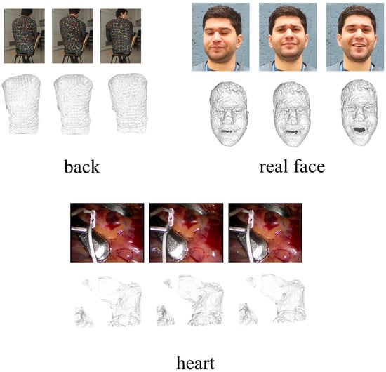
Figure 5.
This figure provides a comprehensive visualization of the reconstruction results obtained from datasets devoid of ground truth values. The datasets in focus encompass the Back dataset, Real Face dataset, and Heart dataset. Within the figure, the original images are situated above, while the corresponding reconstruction results are showcased below. The primary aim of this visual representation is to offer a precise and elaborate depiction of the reconstruction process’s performance and accuracy concerning these datasets, especially considering the absence of ground truth values.
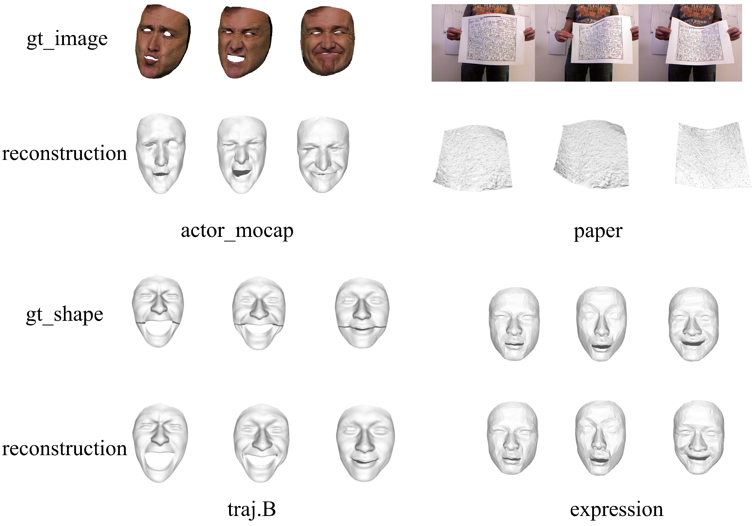
By experimenting with real sequence datasets, the effective simulation of non-rigid object deformation in real-world scenarios becomes possible. This is crucial in validating the practicality and adaptability of the proposed method. Furthermore, qualitative results for four additional datasets: Actor Mocap, Expressions, Traj.B, and Paper, are analyzed, and these results are depicted in Figure 6, providing further insights into the method’s performance.
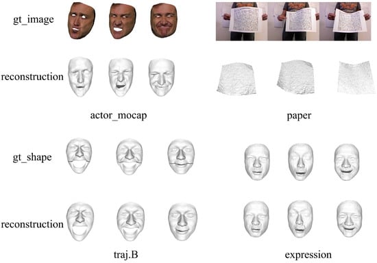
Figure 6.
This figure provides a visual representation of the qualitative analysis of the four datasets previously subjected to quantitative assessment, namely, Actor Mocap, Paper, Traj.B, and Expressions. In the case of the Actor Mocap and Paper datasets, the original images are accompanied by the corresponding reconstruction results displayed beneath each image. Conversely, the Traj.B and Expressions datasets exclusively offer ground truth obj format files, with their respective reconstruction results presented below.
4.3. Module Analysis
4.3.1. Multilayer Linear Module Evaluation
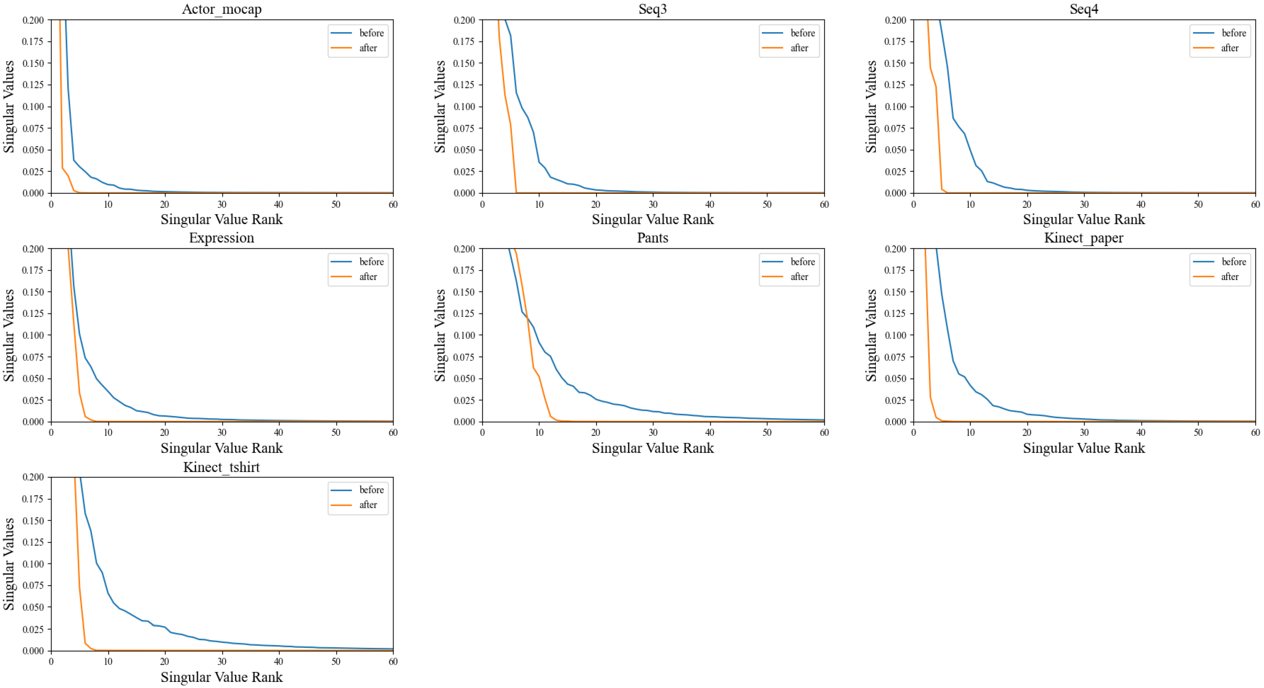
To impose implicit regularization on the acquired feature representation, a linear module is integrated, devoid of activation functions or bias terms. This linear module’s role is to diminish the rank of the feature representation, consequently introducing dimensionality constraints to the potential space. Employing a methodology elucidated in a prior study [12], the rank of the covariance matrix linked with the feature representation is computed both before and after the application of the linear module. This calculation serves as an indicator of the dimensionality of the acquired potential space. The experimental results are depicted in Figure 7.
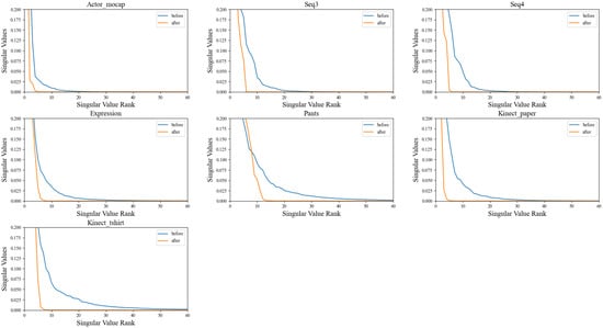
Figure 7.
A comparison of the rank of covariance matrices corresponding to feature representations before and after passing through multilayer linear modules is depicted in the figure. The illustration highlights the influence of multilayer linear modules on the dimensionality of feature representations. It achieves this by comparing the rank of covariance matrices at two critical junctures in the processing pipeline: before the feature input to the modules and after the feature output from the modules.
From the observations in Figure 7, it is evident that the rank of the covariance matrix is significantly decreased after processing with the linear module. The rank of the covariance matrix of the latent variables reflects the linear correlation among them. Hence, a lower rank indicates a higher correlation between each sample in the batch, implying that the data lie in a lower-dimensional space. This outcome aligns with expectations, notably showcasing implicit regularization without the imposition of additional constraints, achieved solely through the introduction of the linear module.
To further validate the effectiveness of the linear module, ablation experiments are performed. The linear module is removed, and the network is retrained. Subsequently, the of the new model on each dataset is computed, serving as the baseline result. Detailed outcomes of these ablation experiments are showcased in Table 6.
Table 6.
Ablation experiment results of obtained from multilayer linear module variations across different datasets.
The effects of linear modules can be further elucidated to provide a deeper understanding of them. The introduction of linear modules, devoid of activation functions and bias terms, yields several phenomena that contribute to the reduction of the rank of the feature representation and the constraint of data within a lower-dimensional potential space. These phenomena can be explained as follows:
- Implicit low-rank representation: The incorporation of linear modules can be viewed as an inherent constraint for attaining a low-rank representation of the features. This reduction in the rank of the feature representation serves to constrain the linear correlations among features, thereby facilitating a more efficient data representation within a lower-dimensional potential space.
- Feature dimensionality reduction and denoising: The role of the linear module can be likened to the procedures of dimensionality reduction and denoising. By reducing the dimensionality of the feature representation, superfluous details and noise are discarded, thereby bolstering the model’s capacity to capture crucial information within the data. Consequently, this enhances the model’s robustness and its ability to generalize effectively.
- Solution space of the optimization problem: The introduction of linear modules has the potential to alter the solution space of the optimization problem. These modules impose constraints on the rank of the feature representation, guiding the optimization problem to be solved within a more simplified solution space. This alteration leads to improved convergence and stability during the training process.
- Tightness of data representation: The reduction of the rank in the feature representation encourages a more compact modeling of the data in a representative feature space. This aids in reducing the redundancy of the representation and extracting more meaningful features, ultimately enhancing the accuracy and interpretability of the reconstruction results.
4.3.2. Multiple Self-Attention Module Evaluation
A multi-attention module design is incorporated to sequentially extract and encode feature information from the input sequence, with the objective of creating a more meaningful and smooth potential space. The T-SNE algorithm is utilized to reduce and represent the feature representations both before (Figure 8) and after processing by the self-attention modules (Figure 9). In these visualizations, each point on the graph corresponds to a frame within the sequence, and its color signifies its temporal order. Ideally, these points should exhibit a continuous trajectory in accordance with their temporal sequence.
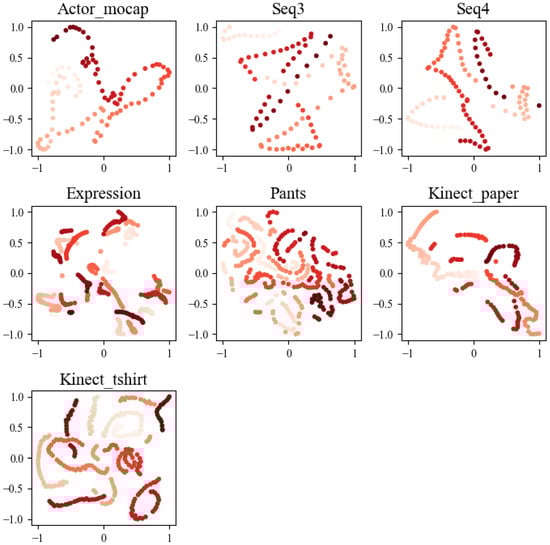
Figure 8.
The visualization results depict the outcome of T-SNE dimensionality reduction, transforming the feature vector into a 2D latent space before passing through the self-attention layer. Each point represents a frame within the sequence, and the color corresponds to its temporal order. These visualizations serve to provide a clear representation of how the data is distributed in this lower-dimensional latent space.
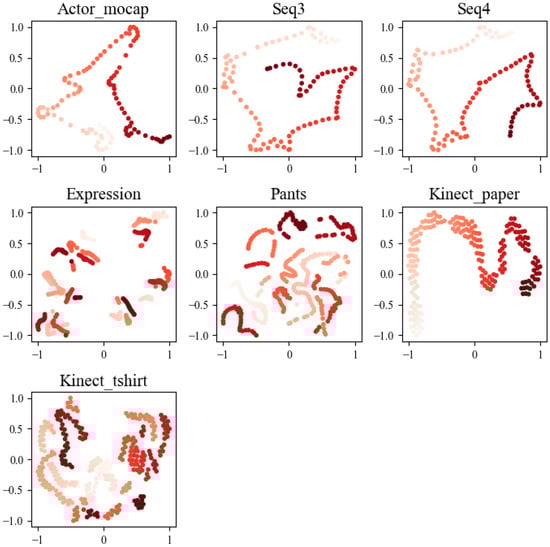
Figure 9.
The visualization results depict the outcome of T-SNE dimensionality reduction for the feature vector after passing through the self-attention layer. Each point on the graph represents a frame within the sequence, with color coding indicating its temporal order. These visualizations are instrumental in elucidating how data points are distributed in a 2D latent space following processing by the self-attention modules.
After analyzing the visualization results, it becomes evident that the feature representation, following its interaction with the self-attention module, exhibits a more coherent and well-defined trajectory structure. This observation underscores the module’s effectiveness in capturing the intricate motion and deformation characteristics inherent to non-rigid objects when encoding sequential features. Consequently, the potential space demonstrates more meaningful and smoother properties. In contrast, the unprocessed feature representation showcases scattered or fragmented trajectories within the graph. This stark difference further reaffirms the positive impact of the self-attention module in the approach, enhancing the representation of sequential features and facilitating the accurate modeling of the structural complexities involved in motion recovery for non-rigid objects.
Moreover, ablation experiments were performed, involving the removal of the self-attention module and subsequent retraining of the network to establish the baseline model, termed Baseline-A. The comparison of results, as depicted in Table 7, reveals a noteworthy increase in errors for the baseline model across all datasets. This outcome signifies that the network struggles to acquire a proficient feature representation when devoid of the self-attention module, leading to a marked deterioration in model performance. Such findings emphasize the pivotal role and effectiveness of the self-attention module within this approach.
Table 7.
Ablation experiment results of obtained from multiple self-attention module variations across different datasets.
4.3.3. Loss Function Evaluation
In addition to the strong constraint of reprojection loss in the NRSFM problem, the energy function proposed here includes a dedicated temporal smoothing term. This term specifically focuses on controlling the level of deformation between neighboring frames, enhancing the temporal coherence and smoothness of reconstructed sequences. Notably, some related studies, such as N-NRSFM [6] and DST-NRSFM [42], have explored the incorporation of an extra spatial smoothing loss term to promote shape smoothness. While this has the potential to further improve reconstruction performance, it also introduces added complexity to the network optimization process and relies on the availability of shape templates provided by the dataset.
To assess the impact of the time-smoothing loss in the network architecture, ablation experiments were conducted. A baseline model, referred to as Baseline-B, was trained using solely reprojection errors as the training objective. Subsequently, the performance of this baseline model was compared with the method under consideration.
The results presented in Table 8 unequivocally reveal the enhanced performance of the method in comparison to the baseline model concerning reconstruction error across most datasets. Nevertheless, it is important to note that the introduction of the time-smoothing loss term slightly elevates the reconstruction error on the Traj.B dataset. Specifically, when the model is exclusively trained with reprojection error, it attains an error of 0.017, outperforming the error of 0.019 achieved when the time-smoothing loss term is included. This observation suggests that for datasets characterized by relatively lower levels of deformation, like Traj.B, the proposed method can yield satisfactory results through training solely with the reprojection error.
Table 8.
Ablation experiment results of obtained from temporal constrain variations across different datasets.
The influence of the time-smoothing loss term is somewhat limited when applied to datasets with minimal deformation. However, its significance becomes more pronounced in datasets with substantial deformation, as exemplified by the Kinect dataset. In these scenarios, a marked improvement in results is evident. The incorporation of the time-smoothing loss term plays a pivotal role in augmenting the temporal coherence and continuity of the reconstructed non-rigid object motion. Consequently, this enhancement results in a more precise and visually pleasing reconstruction.
These findings imply that the effectiveness of the time-smoothing loss term in the energy function is influenced by the level of deformation present in the dataset. When the dataset exhibits less deformation, training with reprojection error alone can already yield satisfactory results. However, for datasets with more pronounced deformation, the incorporation of the time-smoothing loss term becomes crucial for achieving significant improvements in reconstruction accuracy.
5. Conclusions
In summary, this innovative neural network approach addresses the challenging problem of dense NRSFM. By leveraging multiple self-attention layers and temporal smoothness constraints, the method transforms 2D sequence images into high-dimensional 3D structures, achieving implicit regularization through a novel linear layer.
The results demonstrate the method’s effectiveness in handling dense NRSFM problems, outperforming existing approaches on various benchmark datasets. Accurate 3D shape recovery for non-rigid objects is achieved, contributing significantly to the field of computer vision. Importantly, it is noted that excessively long input sequences may lead to method ineffectiveness due to the exponential increase in parameters caused by self-attention mechanisms.
As a potential avenue for future research, exploring the use of image sequences as input, instead of measurement matrices, can facilitate the development of an end-to-end pipeline for generating 3D structures directly from images. This approach offers exciting possibilities for further exploration.
Author Contributions
Conceptualization, Y.W., W.H. and M.J.; methodology, Y.W., W.H. and D.X.; software, D.X.; validation, Y.W., W.H. and M.J.; formal analysis, Y.W. and D.X.; investigation, D.X. and X.Y.; data curation, D.X. and X.Y.; writing—original draft preparation, D.X. and W.H.; writing—review and editing, Y.W., W.H. and D.X.; visualization, Y.W. and D.X.; supervision, Y.W. and W.H. All authors have read and agreed to the published version of the manuscript.
Funding
This research is supported by the Natural Science Foundation of Zhejiang Province (LZ20F020003, LZ21F020003, LSZ19F010001, LY17F020003), and the National Natural Science Foundation of China (61272311, 61672466).
Institutional Review Board Statement
Not applicable.
Informed Consent Statement
Not applicable.
Data Availability Statement
The data are not publicly available due to privacy.
Conflicts of Interest
The authors declare no conflict of interest.
References
- Wang, C.; Lucey, S. Paul: Procrustean autoencoder for unsupervised lifting. In Proceedings of the IEEE/CVF Conference on Computer Vision and Pattern Recognition, Online, 19–25 June 2021; pp. 434–443. [Google Scholar]
- Russell, C.; Fayad, J.; Agapito, L. Dense non-rigid structure from motion. In Proceedings of the 2012 Second International Conference on 3D Imaging, Modeling, Processing, Visualization & Transmission, Li’ege, Belgium, 3–5 December 2012; pp. 509–516. [Google Scholar]
- Golyanik, V.; Stricker, D. Dense batch non-rigid structure from motion in a second. In Proceedings of the 2017 IEEE Winter Conference on Applications of Computer Vision (WACV), Santa Rosa, CA, USA, 24–31 March 2017; pp. 254–263. [Google Scholar]
- Kumar, S.; Van Gool, L. Organic priors in non-rigid structure from motion. In Proceedings of the European Conference on Computer Vision, Tel Aviv, Israel, 23–27 October 2022; Springer: Berlin/Heidelberg, Germany, 2022; pp. 71–88. [Google Scholar]
- Song, J.; Patel, M.; Jasour, A.; Ghaffari, M. A closed-form uncertainty propagation in non-rigid structure from motion. IEEE Robot. Autom. Lett. 2022, 7, 6479–6486. [Google Scholar] [CrossRef]
- Sidhu, V.; Tretschk, E.; Golyanik, V.; Agudo, A.; Theobalt, C. Neural dense non-rigid structure from motion with latent space constraints. In Proceedings of the Computer Vision–ECCV 2020: 16th European Conference, Glasgow, UK, 23–28 August 2020; Part XVI 16. Springer: Berlin/Heidelberg, Germany, 2020; pp. 204–222. [Google Scholar]
- Agudo, A.; Montiel, J.; Agapito, L.; Calvo, B. Online Dense Non-Rigid 3D Shape and Camera Motion Recovery. In Proceedings of the BMVC, Nottingham, UK, 1–5 September 2014. [Google Scholar]
- Garg, R.; Roussos, A.; Agapito, L. Dense variational reconstruction of non-rigid surfaces from monocular video. In Proceedings of the IEEE Conference on Computer Vision and Pattern Recognition, Portland, OR, USA, 23–27 June 2013; pp. 1272–1279. [Google Scholar]
- Kumar, S.; Cherian, A.; Dai, Y.; Li, H. Scalable dense non-rigid structure-from-motion: A grassmannian perspective. In Proceedings of the IEEE Conference on Computer Vision and Pattern Recognition, Salt Lake City, UT, USA, 18–22 June 2018; pp. 254–263. [Google Scholar]
- Tomasi, C.; Kanade, T. Shape and motion from image streams: A factorization method. Proc. Natl. Acad. Sci. USA 1993, 90, 9795–9802. [Google Scholar] [CrossRef]
- Deng, H.; Zhang, T.; Dai, Y.; Shi, J.; Zhong, Y.; Li, H. Deep Non-rigid Structure-from-Motion: A Sequence-to-Sequence Translation Perspective. arXiv 2022, arXiv:2204.04730. [Google Scholar]
- Jing, L.; Zbontar, J. Implicit rank-minimizing autoencoder. Adv. Neural Inf. Process. Syst. 2020, 33, 14736–14746. [Google Scholar]
- Bregler, C.; Hertzmann, A.; Biermann, H. Recovering non-rigid 3D shape from image streams. In Proceedings of the IEEE Conference on Computer Vision and Pattern Recognition, CVPR 2000 (Cat. No. PR00662), Hilton Head, SC, USA, 13–15 June 2000; Volume 2, pp. 690–696. [Google Scholar]
- Akhter, I.; Sheikh, Y.; Khan, S.; Kanade, T. Nonrigid structure from motion in trajectory space. In Proceedings of the Advances in Neural Information Processing Systems 21 (NIPS 2008), Vancouver, BC, Canada, 8–10 December 2008; Volume 21. [Google Scholar]
- Torresani, L.; Hertzmann, A.; Bregler, C. Nonrigid structure-from-motion: Estimating shape and motion with hierarchical priors. IEEE Trans. Pattern Anal. Mach. Intell. 2008, 30, 878–892. [Google Scholar] [CrossRef]
- Rabaud, V.; Belongie, S. Re-thinking non-rigid structure from motion. In Proceedings of the 2008 IEEE Conference on Computer Vision and Pattern Recognition, Anchorage, AK, USA, 23–28 June 2008; pp. 1–8. [Google Scholar]
- Gotardo, P.F.; Martinez, A.M. Kernel non-rigid structure from motion. In Proceedings of the 2011 International Conference on Computer Vision, Barcelona, Spain, 6–13 November 2011; pp. 802–809. [Google Scholar]
- Hamsici, O.C.; Gotardo, P.F.; Martinez, A.M. Learning spatially-smooth mappings in non-rigid structure from motion. In Proceedings of the Computer Vision–ECCV 2012: 12th European Conference on Computer Vision, Florence, Italy, 7–13 October 2012; Part IV 12. Springer: Berlin/Heidelberg, Germany, 2012; pp. 260–273. [Google Scholar]
- Kumar, S. Jumping manifolds: Geometry aware dense non-rigid structure from motion. In Proceedings of the IEEE/CVF Conference on Computer Vision and Pattern Recognition, Long Beach, CA, USA, 15–20 June 2019; pp. 5346–5355. [Google Scholar]
- Dai, Y.; Li, H.; He, M. A simple prior-free method for non-rigid structure-from-motion factorization. Int. J. Comput. Vis. 2014, 107, 101–122. [Google Scholar] [CrossRef]
- Ansari, M.D.; Golyanik, V.; Stricker, D. Scalable dense monocular surface reconstruction. In Proceedings of the 2017 International Conference on 3D Vision (3DV), Qingdao, China, 10–12 October 2017; pp. 78–87. [Google Scholar]
- Lee, M.; Cho, J.; Choi, C.H.; Oh, S. Procrustean normal distribution for non-rigid structure from motion. In Proceedings of the IEEE Conference on Computer Vision and Pattern Recognition, Portland, OR, USA, 23–27 June 2013; pp. 1280–1287. [Google Scholar]
- Gower, J.C. Generalized procrustes analysis. Psychometrika 1975, 40, 33–51. [Google Scholar] [CrossRef]
- Lee, M.; Choi, C.H.; Oh, S. A procrustean Markov process for non-rigid structure recovery. In Proceedings of the IEEE Conference on Computer Vision and Pattern Recognition, Columbus, OH, USA, 23–28 June 2014; pp. 1550–1557. [Google Scholar]
- Kong, C.; Lucey, S. Deep non-rigid structure from motion. In Proceedings of the IEEE/CVF International Conference on Computer Vision, Seoul, Republic of Korea, 27 October–2 November 2019; pp. 1558–1567. [Google Scholar]
- Papyan, V.; Romano, Y.; Elad, M. Convolutional neural networks analyzed via convolutional sparse coding. J. Mach. Learn. Res. 2017, 18, 2887–2938. [Google Scholar]
- Novotny, D.; Ravi, N.; Graham, B.; Neverova, N.; Vedaldi, A. C3dpo: Canonical 3d pose networks for non-rigid structure from motion. In Proceedings of the IEEE/CVF International Conference on Computer Vision, Seoul, Republic of Korea, 27 October–2 November 2019; pp. 7688–7697. [Google Scholar]
- Cha, G.; Lee, M.; Oh, S. Unsupervised 3d reconstruction networks. In Proceedings of the IEEE/CVF International Conference on Computer Vision, Seoul, Republic of Korea, 27 October–2 November 2019; pp. 3849–3858. [Google Scholar]
- Park, S.; Lee, M.; Kwak, N. Procrustean regression networks: Learning 3d structure of non-rigid objects from 2d annotations. In Proceedings of the European Conference on Computer Vision, Online, 23–28 August 2020; Springer: Berlin/Heidelberg, Germany, 2020; pp. 1–18. [Google Scholar]
- Kong, C.; Lucey, S. Deep non-rigid structure from motion with missing data. IEEE Trans. Pattern Anal. Mach. Intell. 2020, 43, 4365–4377. [Google Scholar] [CrossRef] [PubMed]
- Wang, C.; Lin, C.H.; Lucey, S. Deep nrsfm++: Towards unsupervised 2d-3d lifting in the wild. In Proceedings of the 2020 International Conference on 3D Vision (3DV), Fukuoka, Japan, 25–28 November 2020; pp. 12–22. [Google Scholar]
- Ma, Z.; Li, K.; Li, Y. Self-supervised method for 3D human pose estimation with consistent shape and viewpoint factorization. Appl. Intell. 2023, 53, 3864–3876. [Google Scholar] [CrossRef]
- Zeng, H.; Dai, Y.; Yu, X.; Wang, X.; Yang, Y. PR-RRN: Pairwise-regularized residual-recursive networks for non-rigid structure-from-motion. In Proceedings of the IEEE/CVF International Conference on Computer Vision, Montreal, QC, Canada, 10–17 October 2021; pp. 5600–5609. [Google Scholar]
- Chen, C.H.; Tyagi, A.; Agrawal, A.; Drover, D.; Mv, R.; Stojanov, S.; Rehg, J.M. Unsupervised 3d pose estimation with geometric self-supervision. In Proceedings of the IEEE/CVF Conference on Computer Vision and Pattern Recognition, Long Beach, CA, USA, 16–20 June 2019; pp. 5714–5724. [Google Scholar]
- Drover, D.; MV, R.; Chen, C.H.; Agrawal, A.; Tyagi, A.; Phuoc Huynh, C. Can 3d pose be learned from 2d projections alone? In Proceedings of the European Conference on Computer Vision (ECCV) Workshops, Munich, Germany, 8–14 September 2018. [Google Scholar]
- Kudo, Y.; Ogaki, K.; Matsui, Y.; Odagiri, Y. Unsupervised adversarial learning of 3d human pose from 2d joint locations. arXiv 2018, arXiv:1803.08244. [Google Scholar]
- Wandt, B.; Rosenhahn, B. Repnet: Weakly supervised training of an adversarial reprojection network for 3d human pose estimation. In Proceedings of the IEEE/CVF Conference on Computer Vision and Pattern Recognition, Long Beach, CA, USA, 16–20 June 2019; pp. 7782–7791. [Google Scholar]
- Wang, C.; Li, X.; Pontes, J.K.; Lucey, S. Neural prior for trajectory estimation. In Proceedings of the IEEE/CVF Conference on Computer Vision and Pattern Recognition, New Orleans, LA, USA, 19–24 June 2022; pp. 6532–6542. [Google Scholar]
- Golyanik, V.; Jonas, A.; Stricker, D. Consolidating segmentwise non-rigid structure from motion. In Proceedings of the 2019 16th International Conference on Machine Vision Applications (MVA), Tokyo, Japan, 27–31 May 2019; pp. 1–6. [Google Scholar]
- Agudo, A.; Moreno-Noguer, F. A scalable, efficient, and accurate solution to non-rigid structure from motion. Comput. Vis. Image Underst. 2018, 167, 121–133. [Google Scholar] [CrossRef]
- Wang, Y.; Peng, X.; Huang, W.; Wang, M. A convolutional neural network for nonrigid structure from motion. Int. J. Digit. Multimed. Broadcast. 2022, 2022, 3582037. [Google Scholar] [CrossRef]
- Wang, Y.; Wang, M.; Huang, W.; Ye, X.; Jiang, M. Deep Spatial-Temporal Neural Network for Dense Non-Rigid Structure from Motion. Mathematics 2022, 10, 3794. [Google Scholar] [CrossRef]
- Tewari, A.; Bernard, F.; Garrido, P.; Bharaj, G.; Elgharib, M.; Seidel, H.P.; Pérez, P.; Zollhofer, M.; Theobalt, C. Fml: Face model learning from videos. In Proceedings of the IEEE/CVF Conference on Computer Vision and Pattern Recognition, Long Beach, CA, USA, 16–20 June 2019; pp. 10812–10822. [Google Scholar]
- Gotardo, P.F.; Martinez, A.M. Non-rigid structure from motion with complementary rank-3 spaces. In Proceedings of the CVPR, Colorado Springs, CO, USA, 20–25 June 2011; pp. 3065–3072. [Google Scholar]
- Agudo, A.; Moreno-Noguer, F. Global model with local interpretation for dynamic shape reconstruction. In Proceedings of the 2017 IEEE Winter Conference on Applications of Computer Vision (WACV), Santa Rosa, CA, USA, 24–31 March 2017; pp. 264–272. [Google Scholar]
- Paladini, M.; Del Bue, A.; Xavier, J.; Agapito, L.; Stošić, M.; Dodig, M. Optimal metric projections for deformable and articulated structure-from-motion. Int. J. Comput. Vis. 2012, 96, 252–276. [Google Scholar] [CrossRef]
- Dai, Y.; Deng, H.; He, M. Dense non-rigid structure-from-motion made easy—A spatial-temporal smoothness based solution. In Proceedings of the 2017 IEEE International Conference on Image Processing (ICIP), Beijing, China, 17–20 September 2017; pp. 4532–4536. [Google Scholar]


Disclaimer/Publisher’s Note: The statements, opinions and data contained in all publications are solely those of the individual author(s) and contributor(s) and not of MDPI and/or the editor(s). MDPI and/or the editor(s) disclaim responsibility for any injury to people or property resulting from any ideas, methods, instructions or products referred to in the content. |
© 2023 by the authors. Licensee MDPI, Basel, Switzerland. This article is an open access article distributed under the terms and conditions of the Creative Commons Attribution (CC BY) license (https://creativecommons.org/licenses/by/4.0/).