
ADQE: Obtain Better Deep Learning Models by Evaluating the Augmented Data Quality Using Information Entropy


Abstract
:1. Introduction
- In this paper, we design and implement a data enhancement quality evaluation method, which can optimize and generate large-scale, high-quality data sets by disassembling and balancing the quality dimensions of data sets.
- This paper discusses the choice of mathematical tools for statistical analysis of data dimensions, and determines that information entropy is more suitable than other methods for evaluating the information content of data.
- This paper extensively evaluates the proposed method on various data augmentation techniques, datasets, and models. There is a strong correlation between the experimental results of the deep learning model and the evaluation results of the method, which shows that the method can improve the performance of the model on related tasks by evaluating the data enhancement quality.
2. Methods
2.1. Preliminaries
2.1.1. Deep Learning
2.1.2. Data Augmentation
2.1.3. Benefits of Data Augmentation
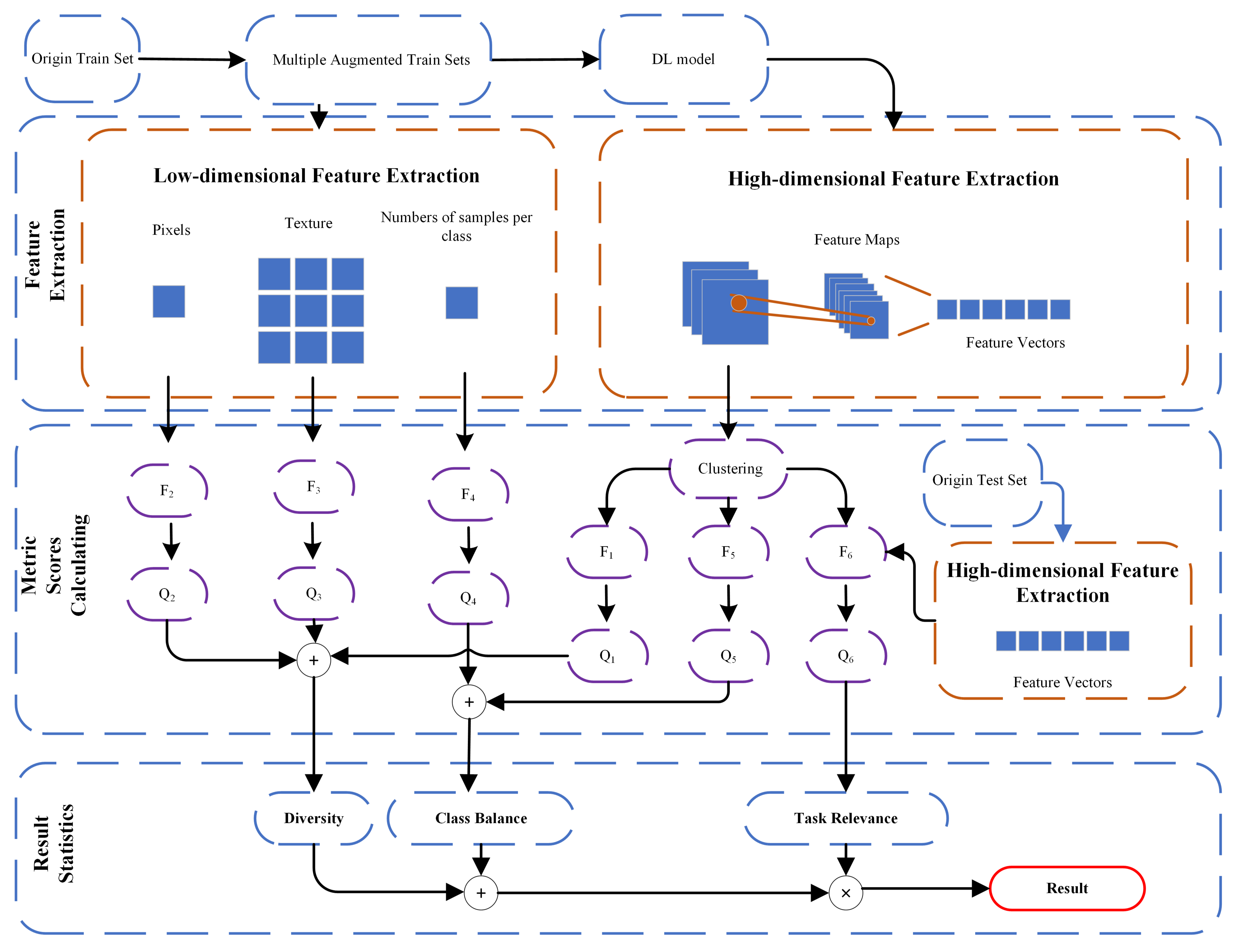
2.2. The Overall Framework
| Algorithm 1: Calculation of all augmented datasets evaluations. |
Data: The collection of augmented datasets , A test dataset , DL model Result: the quality metric of the augmented dataset Q |
 |
2.3. Feature Extraction
2.3.1. Feature Selection
2.3.2. Clustering
2.4. Metric Scores Calculating
2.4.1. Diversity
| Algorithm 2: Rapid calculation of diversity by clustering. |
Data: A training dataset , dataset size , DL model Result: Diversity Metric Scores |
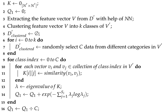 |
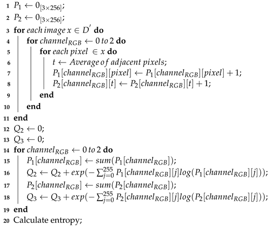
| Algorithm 3: The calculation of image datasets’ color and brightness space. |
Data: A training dataset Result: Diversity Metric Scores and |
 |
2.4.2. Class Balance
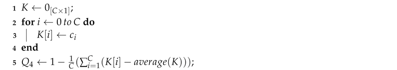
| Algorithm 4: The calculation of quantity balance between classes. |
Data: A training dataset , The number of classes C Result: Class Balance Metric Scores |
 |
| Algorithm 5: The calculation of features balance between classes. |
Data: A training dataset Result: Class Balance Metric Scores |
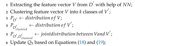 |
2.4.3. Task Relevance
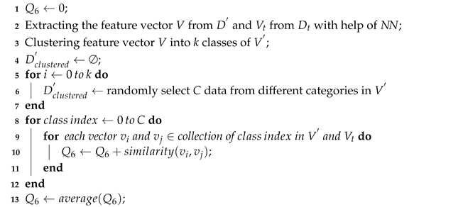
| Algorithm 6: Rapid calculation of task relevance by clustering. |
Data: A training dataset , dataset size , The number of classes C, A test dataset , test dataset size , DL model Result: Task Relevance Metric Scores |
 |
2.5. Result Statistics
3. Experimental
3.1. Datasets and Data Augmentation
3.2. Baseline
3.3. Evaluation Index
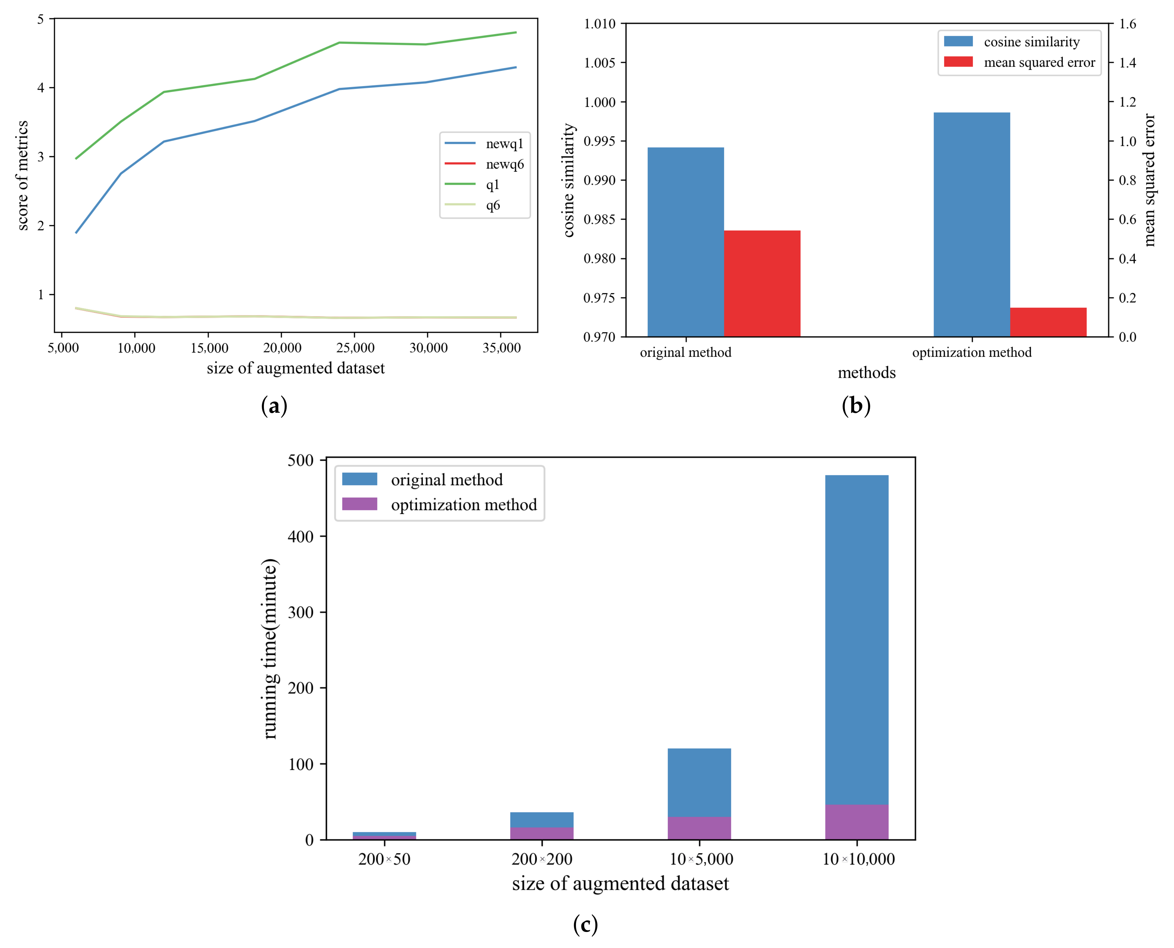
3.4. Ablation Study
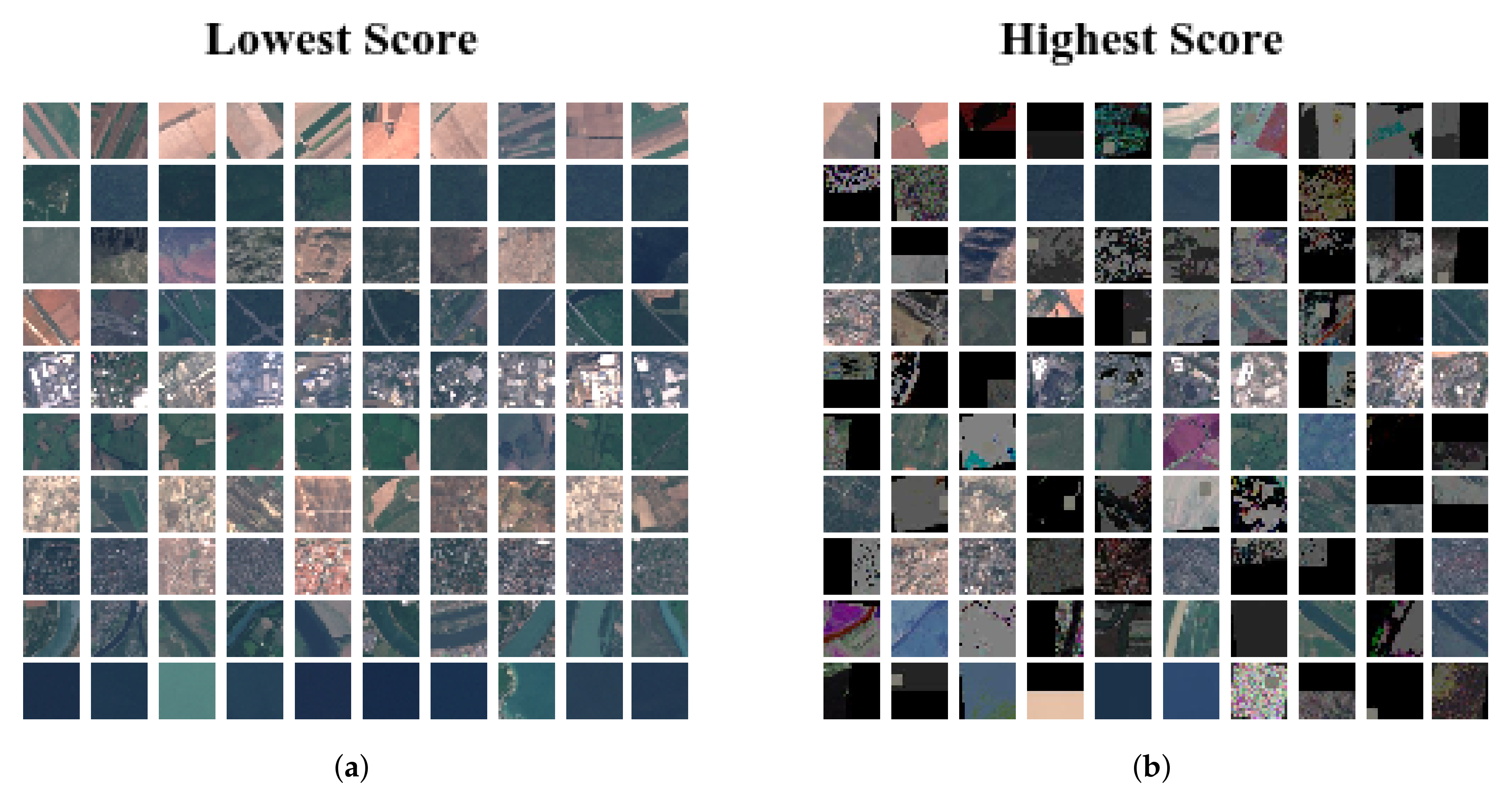
3.5. Case Study
4. Results and Discussion
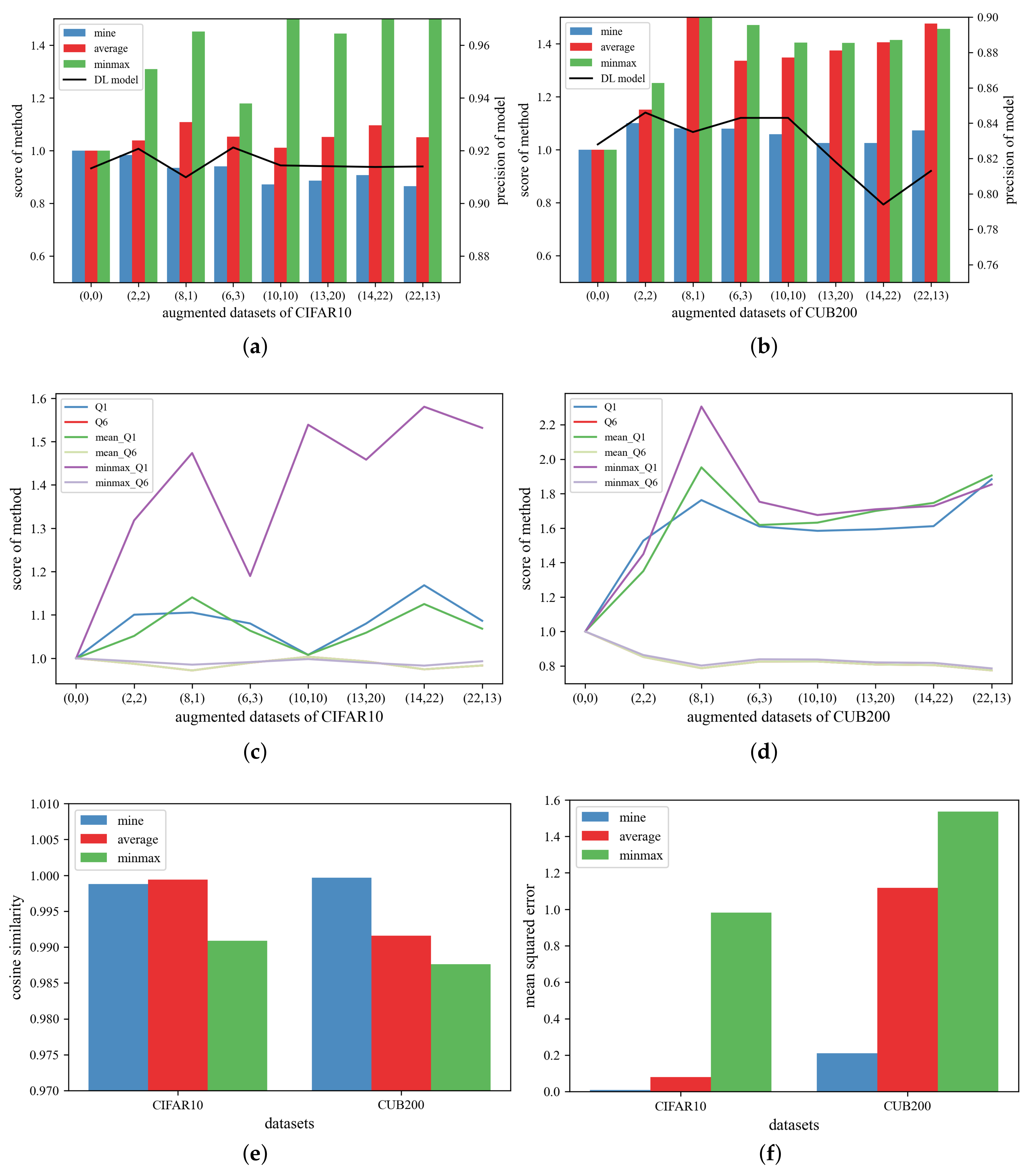
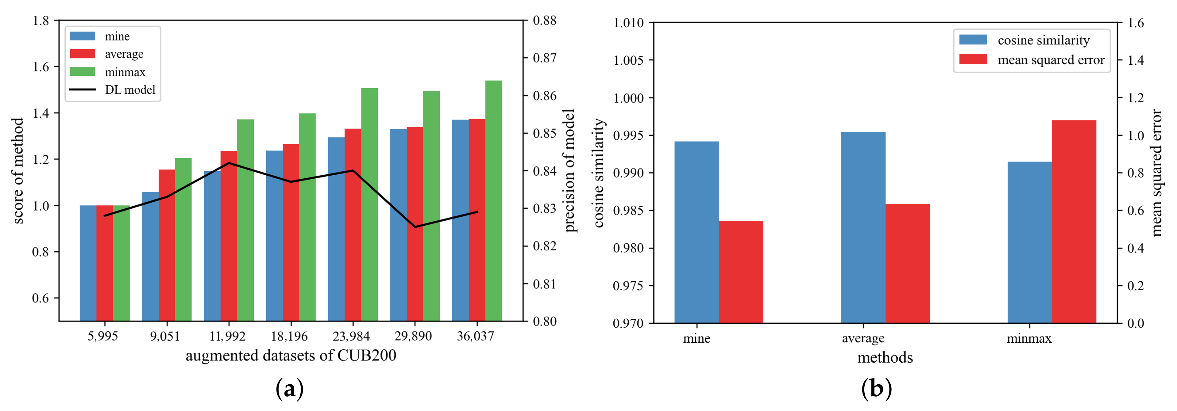
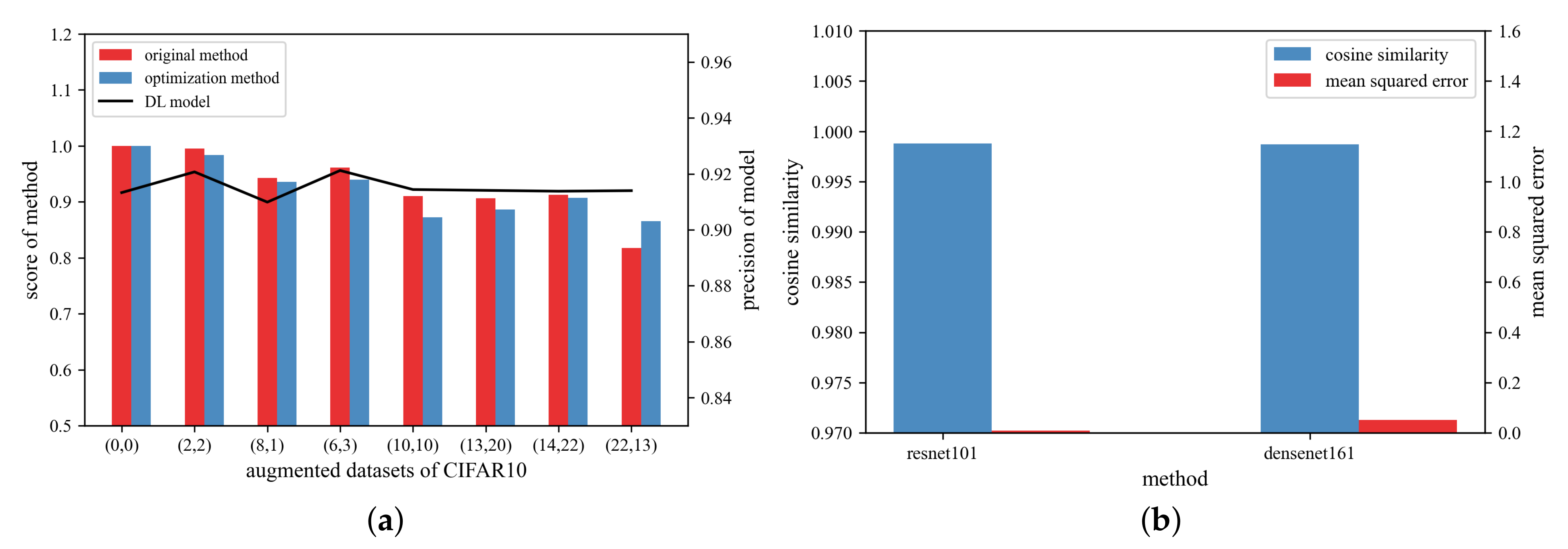
4.1. Results of Comparative Experiments
4.2. Results of Ablation Experiments
4.3. Applicability and Potential Applications
5. Conclusions
Author Contributions
Funding
Data Availability Statement
Acknowledgments
Conflicts of Interest
References
- Zhang, T.; Chen, J.; Li, F.; Zhang, K.; Lv, H.; He, S.; Xu, E. Intelligent fault diagnosis of machines with small & imbalanced data: A state-of-the-art review and possible extensions. ISA Trans. 2022, 119, 152–171. [Google Scholar] [PubMed]
- Chlap, P.; Min, H.; Vandenberg, N.; Dowling, J.; Holloway, L.; Haworth, A. A review of medical image data augmentation techniques for deep learning applications. J. Med. Imaging Radiat. Oncol. 2021, 65, 545–563. [Google Scholar] [CrossRef] [PubMed]
- Silver, D.; Hubert, T.; Schrittwieser, J.; Antonoglou, I.; Lai, M.; Guez, A.; Lanctot, M.; Sifre, L.; Kumaran, D.; Graepel, T.; et al. A general reinforcement learning algorithm that masters chess, shogi, and Go through self-play. Science 2018, 362, 1140–1144. [Google Scholar] [CrossRef] [PubMed]
- Hao, X.; Liu, L.; Yang, R.; Yin, L.; Zhang, L.; Li, X. A Review of Data Augmentation Methods of Remote Sensing Image Target Recognition. Remote Sens. 2023, 15, 827. [Google Scholar] [CrossRef]
- Chen, Y.; Yang, X.H.; Wei, Z.; Heidari, A.A.; Zheng, N.; Li, Z.; Chen, H.; Hu, H.; Zhou, Q.; Guan, Q. Generative adversarial networks in medical image augmentation: A review. Comput. Biol. Med. 2022, 144, 105382. [Google Scholar] [CrossRef]
- Yang, J.; Guo, X.; Li, Y.; Marinello, F.; Ercisli, S.; Zhang, Z. A survey of few-shot learning in smart agriculture: Developments, applications, and challenges. Plant Methods 2022, 18, 28. [Google Scholar] [CrossRef]
- Maslej-Krešňáková, V.; Sarnovskỳ, M.; Jacková, J. Use of Data Augmentation Techniques in Detection of Antisocial Behavior Using Deep Learning Methods. Future Internet 2022, 14, 260. [Google Scholar] [CrossRef]
- Shorten, C.; Khoshgoftaar, T.M.; Furht, B. Text data augmentation for deep learning. J. Big Data 2021, 8, 101. [Google Scholar] [CrossRef]
- Gong, C.; Wang, D.; Li, M.; Chandra, V.; Liu, Q. Keepaugment: A simple information-preserving data augmentation approach. In Proceedings of the IEEE/CVF Conference on Computer Vision and Pattern Recognition, Nashville, TN, USA, 20–25 June 2021; pp. 1055–1064. [Google Scholar]
- Iwana, B.K.; Uchida, S. An empirical survey of data augmentation for time series classification with neural networks. PLoS ONE 2021, 16, e0254841. [Google Scholar] [CrossRef]
- Zhou, X.; Hu, Y.; Wu, J.; Liang, W.; Ma, J.; Jin, Q. Distribution bias aware collaborative generative adversarial network for imbalanced deep learning in industrial IoT. IEEE Trans. Ind. Inform. 2022, 19, 570–580. [Google Scholar] [CrossRef]
- Bishop, C.M. Training with noise is equivalent to Tikhonov regularization. Neural Comput. 1995, 7, 108–116. [Google Scholar] [CrossRef]
- Hernández-García, A.; König, P. Data augmentation instead of explicit regularization. arXiv 2018, arXiv:1806.03852. [Google Scholar]
- Carratino, L.; Cissé, M.; Jenatton, R.; Vert, J.P. On mixup regularization. arXiv 2020, arXiv:2006.06049. [Google Scholar]
- Shen, R.; Bubeck, S.; Gunasekar, S. Data augmentation as feature manipulation. In Proceedings of the International Conference on Machine Learning, Baltimore, MD, USA, 17–23 July 2022; pp. 19773–19808. [Google Scholar]
- Ilse, M.; Tomczak, J.M.; Forré, P. Selecting data augmentation for simulating interventions. In Proceedings of the International Conference on Machine Learning, Virtual Event, 18–24 July 2021; pp. 4555–4562. [Google Scholar]
- Allen-Zhu, Z.; Li, Y. Feature purification: How adversarial training performs robust deep learning. In Proceedings of the 2021 IEEE 62nd Annual Symposium on Foundations of Computer Science (FOCS), Denver, CO, USA, 7–10 February 2022; pp. 977–988. [Google Scholar]
- Kong, Q.; Chang, X. Rough set model based on variable universe. CAAI Trans. Intell. Technol. 2022, 7, 503–511. [Google Scholar] [CrossRef]
- Zhao, H.; Ma, L. Several rough set models in quotient space. CAAI Trans. Intell. Technol. 2022, 7, 69–80. [Google Scholar] [CrossRef]
- Kusunoki, Y.; Błaszczyński, J.; Inuiguchi, M.; Słowiński, R. Empirical risk minimization for dominance-based rough set approaches. Inf. Sci. 2021, 567, 395–417. [Google Scholar] [CrossRef]
- Chen, S.; Dobriban, E.; Lee, J.H. A group-theoretic framework for data augmentation. J. Mach. Learn. Res. 2020, 21, 9885–9955. [Google Scholar]
- Mei, S.; Misiakiewicz, T.; Montanari, A. Learning with invariances in random features and kernel models. In Proceedings of the Conference on Learning Theory, Boulder, CO, USA, 15–19 August 2021; pp. 3351–3418. [Google Scholar]
- Wand, Y.; Wang, R.Y. Anchoring data quality dimensions in ontological foundations. Commun. ACM 1996, 39, 86–95. [Google Scholar] [CrossRef]
- Abdullah, M.Z.; Arshah, R.A. A review of data quality assessment: Data quality dimensions from user’s perspective. Adv. Sci. Lett. 2018, 24, 7824–7829. [Google Scholar] [CrossRef]
- Firmani, D.; Mecella, M.; Scannapieco, M.; Batini, C. On the meaningfulness of “big data quality”. Data Sci. Eng. 2016, 1, 6–20. [Google Scholar] [CrossRef]
- Jarwar, M.A.; Chong, I. Web objects based contextual data quality assessment model for semantic data application. Appl. Sci. 2020, 10, 2181. [Google Scholar] [CrossRef]
- Sim, K.; Yang, J.; Lu, W.; Gao, X. MaD-DLS: Mean and deviation of deep and local similarity for image quality assessment. IEEE Trans. Multimed. 2020, 23, 4037–4048. [Google Scholar] [CrossRef]
- Senaratne, H.; Mobasheri, A.; Ali, A.L.; Capineri, C.; Haklay, M. A review of volunteered geographic information quality assessment methods. Int. J. Geogr. Inf. Sci. 2017, 31, 139–167. [Google Scholar] [CrossRef]
- Chen, H.; Chen, J.; Ding, J. Data evaluation and enhancement for quality improvement of machine learning. IEEE Trans. Reliab. 2021, 70, 831–847. [Google Scholar] [CrossRef]
- Gosain, A.; Saha, A.; Singh, D. Measuring harmfulness of class imbalance by data complexity measures in oversampling methods. Int. J. Intell. Eng. Inform. 2019, 7, 203–230. [Google Scholar] [CrossRef]
- Bellinger, C.; Sharma, S.; Japkowicz, N.; Zaïane, O.R. Framework for extreme imbalance classification: SWIM—Sampling with the majority class. Knowl. Inf. Syst. 2020, 62, 841–866. [Google Scholar] [CrossRef]
- Li, A.; Zhang, L.; Qian, J.; Xiao, X.; Li, X.Y.; Xie, Y. TODQA: Efficient task-oriented data quality assessment. In Proceedings of the 2019 15th International Conference on Mobile Ad-Hoc and Sensor Networks (MSN), Shenzhen, China, 11–13 December 2019; pp. 81–88. [Google Scholar]
- Delgado-Bonal, A.; Marshak, A. Approximate entropy and sample entropy: A comprehensive tutorial. Entropy 2019, 21, 541. [Google Scholar] [CrossRef]
- Li, Y.; Chao, X.; Ercisli, S. Disturbed-entropy: A simple data quality assessment approach. ICT Express 2022, 8, 309–312. [Google Scholar] [CrossRef]
- Liu, L.; Miao, S.; Liu, B. On nonlinear complexity and Shannon’s entropy of finite length random sequences. Entropy 2015, 17, 1936–1945. [Google Scholar] [CrossRef]
- He, K.; Zhang, X.; Ren, S.; Sun, J. Deep residual learning for image recognition. In Proceedings of the IEEE Conference on Computer Vision and Pattern Recognition, Las Vegas, NV, USA, 27–30 June 2016; pp. 770–778. [Google Scholar]
- Sarfraz, S.; Sharma, V.; Stiefelhagen, R. Efficient parameter-free clustering using first neighbor relations. In Proceedings of the IEEE/CVF Conference on Computer Vision and Pattern Recognition, Long Beach, CA, USA, 15–20 June 2019; pp. 8934–8943. [Google Scholar]
- Friedman, D.; Dieng, A.B. The Vendi Score: A Diversity Evaluation Metric for Machine Learning. arXiv 2022, arXiv:2210.02410. [Google Scholar]
- Mishra, S.P.; Sarkar, U.; Taraphder, S.; Datta, S.; Swain, D.P.; Saikhom, R.; Panda, S.; Laishram, M. Multivariate Statistical Data Analysis- Principal Component Analysis (PCA). Int. J. Livest. Res. 2017, 7, 60–78. [Google Scholar]
- Geirhos, R.; Rubisch, P.; Michaelis, C.; Bethge, M.; Wichmann, F.A.; Brendel, W. ImageNet-trained CNNs are biased towards texture; increasing shape bias improves accuracy and robustness. arXiv 2018, arXiv:1811.12231. [Google Scholar]
- Lore, K.G.; Akintayo, A.; Sarkar, S. LLNet: A deep autoencoder approach to natural low-light image enhancement. Pattern Recognit. 2017, 61, 650–662. [Google Scholar] [CrossRef]
- Yang, Y.; Xu, Z. Rethinking the value of labels for improving class-imbalanced learning. Adv. Neural Inf. Process. Syst. 2020, 33, 19290–19301. [Google Scholar]
- Lin, T.Y.; Goyal, P.; Girshick, R.; He, K.; Dollár, P. Focal loss for dense object detection. In Proceedings of the IEEE International Conference on Computer Vision, Venice, Italy, 22–29 October 2017; pp. 2980–2988. [Google Scholar]
- Xu, Y.; Lu, Y. Adaptive weighted fusion: A novel fusion approach for image classification. Neurocomputing 2015, 168, 566–574. [Google Scholar] [CrossRef]
- Ahmad, S.; Pal, R.; Ganivada, A. Rank level fusion of multimodal biometrics using genetic algorithm. Multimed. Tools Appl. 2022, 81, 40931–40958. [Google Scholar] [CrossRef]
- Nawaz, S.; Calefati, A.; Caraffini, M.; Landro, N.; Gallo, I. Are these birds similar: Learning branched networks for fine-grained representations. In Proceedings of the 2019 International Conference on Image and Vision Computing New Zealand (IVCNZ), Dunedin, New Zealand, 2–4 December 2019; pp. 1–5. [Google Scholar]
- Cubuk, E.D.; Zoph, B.; Shlens, J.; Le, Q.V. Randaugment: Practical automated data augmentation with a reduced search space. In Proceedings of the IEEE/CVF Conference on Computer Vision and Pattern Recognition Workshops, Seattle, WA, USA, 14–19 June 2020; pp. 702–703. [Google Scholar]
- Salimans, T.; Goodfellow, I.; Zaremba, W.; Cheung, V.; Radford, A.; Chen, X. Improved techniques for training gans. In Proceedings of the 30th International Conference on Neural Information Processing Systems, Barcelona, Spain, 5–10 December 2016; pp. 2234–2242. [Google Scholar]


| Mathematical Notation | Description |
|---|---|
| X, Y | The data and labels of the dataset, as well as the input and output space of the model. X and Y represent the original training dataset. and represent the augmented training dataset. and represent the test dataset. |
| x, y | The x denotes an input data and the y denotes a label for the data. The x and y represent the original training dataset. The and represent the augmented training dataset. The and represent the test dataset. |
| P, p | Both represent a probability function that describes the distribution of the sample space. |
| R | It represents the risk function. Its subscripts represent the computational ideas used, empirical and expectation, respectively. |
| Q | It represents a collection of data augmentation quality metrics. Each counts the different dimensions of the data. |
| It represents the pixel of the image data. | |
| D | D denotes the dataset. D represents the original training dataset. represents the augmented training dataset. represents the test dataset. |
| C, | C represents the number of classes in the dataset and represents the number of samples in the ith classes of the training dataset. |
| N | It represents the number of samples in the dataset. N represents the original training dataset. represents the augmented training dataset. represents the test dataset. |
| Quality Metrics | Full Name | Category |
|---|---|---|
| diversity of features | diversity | |
| diversity of textures | ||
| diversity of brightness | ||
| balance of number between class | class balance | |
| balance of features between class | ||
| task relevance | task relevance |
| Baseline | Metrics | Formula |
|---|---|---|
| mean criteria | ||
| minmax criteria | ||
| Dataset | Model | Hyperparameters |
|---|---|---|
| CIFAR10 | densenet161 | Epochs = 90, Init lr = 0.1 divide by 5 at 40th, 60th, 80th, Batchsize = 256, Weight decay = 5 , momentum = 0.9 |
| CUB200 | NtsNet | Epochs = 50, Lr = 0.001, Batchsize = 16, Weight decay = 1 , Momentum = 0.9 |
| Fusion of Quality Metrics | Formula | ||||
|---|---|---|---|---|---|
| 0.9999 * | 0.1357 | 0.9997 | 1.4841 | ||
| 0.9805 | 5.6027 | 0.9721 | 16.5365 | ||
| 0.9727 | 9.7748 | 0.9916 | 98.9535 | ||
| 0.9977 | 0.5363 | 0.9995 | 1.8736 |
| Metrics | ||||||
|---|---|---|---|---|---|---|
| 1 | ||||||
| −0.05 | 1 | |||||
| −0.29 | 0.76 * | 1 | ||||
| 0.81 * | 0.10 | −0.10 | 1 | |||
| −0.19 | 0.62 * | 0.81 * | −0.14 | 1 | ||
| −0.92 ** | 0.02 | 0.24 | −0.57 | 0.07 | 1 |
| Metrics | ||||||
|---|---|---|---|---|---|---|
| 1 | ||||||
| −0.23 | 1 | |||||
| −0.71 * | 0.73 * | 1 | ||||
| 0.76 * | 0.11 | −0.24 | 1 | |||
| −0.71 * | 0.79 * | 0.95 ** | −0.19 | 1 | ||
| −0.97 ** | 0.36 | 0.79 * | −0.66 | 0.8 * | 1 |
Disclaimer/Publisher’s Note: The statements, opinions and data contained in all publications are solely those of the individual author(s) and contributor(s) and not of MDPI and/or the editor(s). MDPI and/or the editor(s) disclaim responsibility for any injury to people or property resulting from any ideas, methods, instructions or products referred to in the content. |
© 2023 by the authors. Licensee MDPI, Basel, Switzerland. This article is an open access article distributed under the terms and conditions of the Creative Commons Attribution (CC BY) license (https://creativecommons.org/licenses/by/4.0/).
Share and Cite
Cui, X.; Li, Y.; Xie, Z.; Liu, H.; Yang, S.; Mou, C. ADQE: Obtain Better Deep Learning Models by Evaluating the Augmented Data Quality Using Information Entropy. Electronics 2023, 12, 4077. https://doi.org/10.3390/electronics12194077
Cui X, Li Y, Xie Z, Liu H, Yang S, Mou C. ADQE: Obtain Better Deep Learning Models by Evaluating the Augmented Data Quality Using Information Entropy. Electronics. 2023; 12(19):4077. https://doi.org/10.3390/electronics12194077
Chicago/Turabian StyleCui, Xiaohui, Yu Li, Zheng Xie, Hanzhang Liu, Shijie Yang, and Chao Mou. 2023. "ADQE: Obtain Better Deep Learning Models by Evaluating the Augmented Data Quality Using Information Entropy" Electronics 12, no. 19: 4077. https://doi.org/10.3390/electronics12194077
APA StyleCui, X., Li, Y., Xie, Z., Liu, H., Yang, S., & Mou, C. (2023). ADQE: Obtain Better Deep Learning Models by Evaluating the Augmented Data Quality Using Information Entropy. Electronics, 12(19), 4077. https://doi.org/10.3390/electronics12194077