Siamese Trackers Based on Deep Features for Visual Tracking

Abstract

Visual object tracking poses challenges due to deformation of target object appearance, fast motion, brightness change, blocking due to obstacles, etc. In this paper, a Siamese network that is configured using a convolutional neural network is proposed to improve tracking accuracy and robustness. Object tracking accuracy is dependent on features that can well represent objects. Thus, we designed a convolutional neural network structure that can preserve feature information that is produced in the previous layer to extract spatial and semantic information. Features are extracted from the target object and search area using a Siamese network, and the extracted feature map is input into the region proposal network, where fast Fourier-transform convolution is applied. The feature map produces a probability score for the presence of an object region and an object in a region, where the similarities are high to search the target. The network was trained with a video dataset called ImageNet Large Scale Visual Recognition Challenge. In the experiment, quantitative and qualitative evaluations were conducted using the object-tracking benchmark dataset. The evaluation results indicated competitive results for some video attributes through various experiments. By conducting experiments, the proposed method achieved competitive results for some video attributes, with a success metric of 0.632 and a precision metric of 0.856 as quantitative values.

1. Introduction

Visual object tracking (VOT) is one of the popular research subjects in the computer vision field due to the advantages that can be applied to visual-based application programs, such as factory automation monitoring, autonomous driving, intruder monitoring, and drone work [1,2,3,4]. VOT is regarded as the most challenging and fundamental field because it has to steadily search and track a specific target in video frames. The general VOT process serves to track a target object using a bounding box, which is given in the first frame [5,6,7]. However, information that is obtained from the first frame is not sufficient to track a target object that is present in all frames. With a lack of feature information, object tracking is likely to fail [8,9]. Thus, high-level feature extraction is needed to represent objects well.

Although studies on object tracking have been conducted over the past decade, object tracking is still difficult due to many shortcomings in videos that capture the real world, such as shape conversion, illumination variation, and occlusion. The success of object tracking is dependent on how the information representing objects can robustly represent objects against various problems. Because of this, various approaches have been proposed to solve these problems in object tracking. The existing appearance-model-based tracking method employs a creation or identification model to separate the foreground and background [10].

This method depends on features created using hand-crafted methods. There are related drawbacks, such as not being able to exhibit the key information of the target object or not responding to a change in appearance robustly. To solve these problems, robust features that can represent the attributes of the target object should be extracted, and an appearance model needs to be created. The appearance model created through this process searches for a target in the image frame region and removes the external noise elements.

The two categories in this study are a generative method that focuses on appearance model creation and a discriminative method. In the generative method, the appearance of the target object is configured through the statistical model using object region information estimated from the previous frame. To maintain appearance information, studies on sparse representation and cellular automata have been conducted [11,12]. In contrast, the discriminative method aims to train a classifier that distinguishes objects and surrounding backgrounds. Studies on support vector machines and multiple instance learning have been conducted for classification [13,14]. However, since such methods employ hand-crafted features such as color histograms, poor information is only extracted, which cannot effectively respond to various changes in environments contained in videos.

Deep learning has shown outstanding results in the field of computer vision by introducing powerful algorithms that can automatically extract and learn complex patterns and features from visual data. By applying deep learning, various advantages can be obtained, such as improved accuracy and robustness through the learning and extraction of hierarchical representations of visual features from large datasets. Additionally, deep-learning models learn end-to-end mappings from raw inputs to outputs, greatly reducing complexity and making the models easy to implement. Deep learning also has scalability, making it suitable for applications beyond computer vision, such as the medical field [15,16]. This scalability allows for the efficient processing of large amounts of data, leveraging the parallel processing capabilities of deep-learning models. As a result, models can be developed to handle increasingly complex tasks and data in various domains.

Recent study methods have focused on deep features based on deep learning, shifting from existing hand-crafted methods. Deep features can be mainly obtained using a convolutional neural network (CNN). Features based on CNNs exhibit good performances in a wide range of visual recognition tasks. Since high-level information can be extracted through the multilayers in a CNN, it is gaining ground as a key method that can overcome the limitations of the tracking algorithm applied via the hand-crafted method. A CNN is trained using a large amount of image data and numerous object class types. Features extracted with a CNN show good performances in representing high-level information and distinguishing objects in various categories. Thus, it is important to use deep features extracted from a CNN for VOT applications.

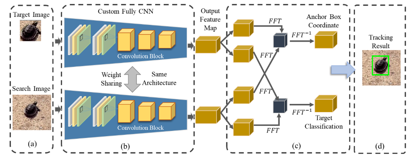
In this paper, unique features of the target object and search region are extracted using a CNN and are used in the object-tracking algorithm by comparing similarities. The tracking problem is regarded as a method to search specific objects inside an image through a similarity comparison rather than considering this as a problem to classify target objects. Image similarity involves a task to compare features of the target object and features of objects that are present in the image plane. Existing CNNs have focused on generalization performance to classify a large number of classes in many types. Because of this, it has caused a low performance for object location identification. Thus, a customized CNN, in which all layers are convolutional, is produced by removing a fully connected layer to preserve object location information. For the similarity comparison, a customized CNN is configured as a Siamese network consisting of a Y-shaped branch network. Since this network is composed of the same weight and shape, similar features are extracted if similar images are input. These features are then input into a fast Fourier-transform (FFT) layer, thus performing a similarity comparison. A region proposal network (RPN) is used to infer a region where the target object is present from the region with the highest similarity.

The main contributions of this paper are as follows. First, we propose a method to increase the robustness of the tracking algorithm by applying FFT to capture global frequency information of the feature map, which can reduce sensitivity to image distortions and noise. Second, we employ a method to leverage the hierarchical characteristics of a Fully Deep CNN, which can effectively utilize both spatially detailed and semantic information. Third, we suggest a region regression technique that examines feature maps generated from various layers and uses deep convolution features and an RPN.

The present paper is organized as follows. In Section 2, studies on VOT are summarized. Section 3 describes a fully convolutional Siamese network for object tracking, while Section 4 describes the experimental results of the proposed tracking algorithm and performance comparison. Lastly, Section 5 presents the conclusion of this study and future research.

2. Related Studies

2.1. Tracking Algorithm Based on Correlation Filter

A correlation filter that is applied to VOT creates an appearance model using features extracted through hand-crafted filters. This appearance model is trained while renewing appearance weights in the partial region of the object obtained in each video frame. Keen attention has been paid to this process due to the high computation efficiency as a result of using FFT. To guarantee the speed of the algorithm, the minimum output sum of the squared error methodology that learns a minimum output sum of a squared error filter on the luminance channel was studied [17]. Furthermore, extended studies to improve the tracking accuracy have been proposed using context learning and a kernelized correlation filter [18,19]. Generally, a correlation filter that exhibits strong signals generates a correlation peak in each interested patch of the frame and produces a low response in the background region. A spatially regularized discriminative correlation filter (SRDCF) tracker imposes constraints on the correlation filter coefficients according to locations using a spatial regularization component in training to induce boundary effects [20]. The MCCTH-Staple tracker combined various types of features and configured various experts through DCF, thus independently tracking the target object with each expert [21]. Channel and spatial reliability concepts were applied to discriminative correlation filter (DCF) tracking, and the spatial reliability map was used for the filter adjustment in the partial region of the target object [22]. Improved kernelized correlation filters employ multichannel features, and they are the most widely used filters because of their overall outstanding performance and high frame-per-second rate [23].

2.2. Tracking Algorithm Based on CNN

CNNs have been used to obtain technical features, being validated in various works as an emerging network with excellent capability in computer vision and pattern recognition, such as image and video classification and object recognition [24,25]. It is important to use features that can be obtained from each convolution layer in the CNN for VOT. Visual representation plays the role of the key element in object tracking. Existing tracking algorithms employ a large number of hand-crafted features to represent a partial space and target shape, such as a color histogram [26,27].

More recently, studies on the application of CNNs’ deep features in tracking algorithms have been conducted. A deep-learning tracker that used a multilayer auto-encoder network was proposed [28]. DeepTrack consists of two-layer CNN classifiers using binary samples, while model updates are conducted via fine adjustment online [29]. Studies on the use of neural networks that learn a target-specific saliency map for tracking have also been conducted [30,31]. A tracking algorithm that adopted hierarchical features that were individually output from the convolution layer in the network was proposed to guarantee the tracking accuracy and robustness of VOT [32].

3. Proposed Method

In this section, the proposed tracking algorithm is described, as shown in Figure 1. The target object and search region images are used for the network input. The main features are extracted from the target object and search region in the Fully Deep CNN. This network is a Siamese network consisting of a Y-shaped branch network. Each feature passes through an FFT layer included in the RPN, thus classifying objects and calculating the bounding box center coordinates.

3.1. Siamese Network with CNN for Feature Extraction

Studies using features obtained with a CNN have been positioned as the key important element in the computer vision area. It is important to use features obtained with a CNN for robust VOT. In a standard CNN, features are extracted using a convolutional layer, and results are produced in a fully connected layer. However, there is a limitation in the fully connected layer from the VOT viewpoint. It is a problem of the disappearance of spatial location information.

Figure 2 shows that spatial information is maintained when only a convolutional layer is used. It is effective to use a fully connected layer because generalization should be performed inside the same class in a simple-class classification problem, and variables such as location information should not change. However, the purpose of VOT is not to infer a specific class but, rather, to infer the location of the target object that is present in a video frame. Thus, it is not appropriate to use a fully connected layer where location information disappears. In this paper, a customized network in which the fully connected layer is removed is developed. By deeply stacking convolutional layers, spatial information is maintained, and semantic information is used, as shown in Figure 2. To configure a deep convolutional layer, a convolutional block consisting of 1 × 1 and 3 × 3 filters was applied. The input feature map was compressed using a 1 × 1 filter, and the feature map was expanded using a 3 × 3 filter. A high-level feature map could be obtained because more convolutional layers could be stacked, even if the same number of parameters was used, by applying a convolutional block.

Figure 3 shows the feature map produced in the visualized convolutional layer. Figure 3a shows the input image, and 3b–d show the output results using the same layer and filter. The figures demonstrate that the output feature map, after passing through the convolutional layer, represented the location information and feature owned by the object. In this paper, a custom-tailored CNN was configured with a Siamese network for feature extraction.

Siamese networks are a type of deep-learning architecture specialized in tasks related to comparing the similarity between two pairs of input data. In particular, it serves as a core method in data-comparison-based applications, such as face recognition and signature verification systems. The fundamental concept of Siamese networks involves training the network on pairs of datapoints to learn a similarity metric between two inputs. A Siamese network encompasses four main features. Firstly, two pairs of data are input to the network in the form of pairs. If the input data type is an image, the reference image and the image to be compared are configured as a pair and fed into the network. Secondly, all parameters of the network are shared with each other. A Siamese network consists of a Y-shaped branch network with two identical structures, as shown in Figure 4. Since a Siamese network employs the same CNN, it is characterized by parameter and weight sharing. Although data pairs are input individually, the same parameters are used throughout the process. Thirdly, data features are extracted through the same network. The structure used for feature extraction may vary depending on the architectural layer that constitutes the network. If similar images are input, a similar feature map is produced. Images pass through the network to extract more detailed features. Lastly, a distance function is utilized to measure the similarity between the features of the extracted data. It quantifies the degree of similarity or distance between features of data pairs extracted from the network. General neural networks train a method to predict multiple classes, whereas a Siamese network can train the comparison of similarity between two images. The proposed architecture of the Siamese network is shown in Figure 5.

Figure 5 shows the network structure used to solve the tracking problem. It was designed by stacking a convolutional block consisting of convolutional layers that included kernels measuring 1 × 1 and 3 × 3 in size to increase the number of kernels that extracted features. The final output feature map in the tracking object region measured 18 × 18 × 256 in size, and the final output feature map in the search region measured 34 × 34 × 256 in size.

Meanwhile, Figure 6 shows the visualized heat map measuring image similarity using the output feature map. The brighter the section, the higher the similarity. This result verifies that the target object region could be approximated. However, we needed to obtain high-level information, such as coordinates, using a feature map to infer an accurate region.

3.2. Region Proposal Network for Estimating Object Area and Coordinates

In Faster R-CNN, an RPN (region proposal network) [33] is introduced to predict bounding box coordinates around objects present in an image. The RPN takes as input a feature map generated via passing the image through a convolutional neural network (CNN). This feature map encodes structural features and spatial information related to target objects. For the object region, feature maps of the target object and search region, which are finally produced in a Siamese network, are used.

Figure 7 shows the anchor box structure that infers coordinates in an RPN. An anchor box is arranged in every cell of the feature map. The number of anchor boxes can be arbitrarily set. It can be advantageous to infer more accurate object regions if the number of anchor boxes whose sizes are different increases. Conversely, as the number of anchor boxes increases, so does the number of computations.

The primary function of the RPN is to predict anchor box coordinates through regression and determine whether an object is present within each anchor box. Each anchor box is defined by four values: center X, center Y, width, and height. The number of anchor boxes varies based on the chosen box scale and aspect ratio. For instance, with a scale of three and an aspect ratio of two, six anchor boxes are generated. Each anchor box is placed individually in each cell of the feature map. Each anchor box is associated with one of three labels. A positive number indicates that there is significant area overlap between the object and the anchor box. A negative number indicates little or no overlap with the object, and −1 is data that do not fall into either the positive or negative categories. Data with −1 labels are ignored during the training process of the RPN to avoid interference.

The RPN performs binary classification to determine whether each anchor box contains an object or not. This classification yields probabilities ranging from 0 to 1. Boxes with probabilities close to 0 are classified as background, while those approaching 1 are considered to contain a substantial portion of an object.

The object existence in the anchor box and the inference of boxes are conducted in the converted frequency domain using FFT. The advantages of applying FFT in convolution are as follows. Firstly, in terms of computational speed, FFT-based convolution exhibits higher computational efficiency compared to traditional spatial domain convolution. This efficiency is particularly pronounced when processing large input data or kernels. While the computational complexity of conventional convolution is $O\left(N^2\right)$, FFT-based convolution reduces it to $O(N\log N)$. Here, N denotes the size of the input data or feature map. Secondly, FFT-based convolution excels in handling large kernels. As the kernel size increases, the computational cost of conventional convolution escalates. In contrast, FFT-based convolution maintains a relatively consistent performance, making it advantageous for operations involving large kernels. Consequently, performance gains can be achieved by integrating both conventional and FFT-based convolutions. Lastly, from the perspective of convolution theory, convolution is equated in the spatial domain to multiplication in the frequency domain. This equivalence offers the advantage of easily modifying and applying algorithms. The convolution in the spatial domain can be simply represented by the Hadamard product in the frequency domain that is obtained through FFT. It is converted into a frequency domain by applying FFT to the feature map of the target object and search region. In the feature map, which is used to determine whether an object is present in the anchor box region, FFT is applied as represented in Equations (1) and (2). In the feature map, which is used to infer the center coordinates of the anchor box, FFT is applied as represented in Equations (3) and (4).

$$T_{cls}\left(u,v\right)=FFT\left(t_{cls}\left(x,y\right)\right)$$

(1)

$$S_{cls}\left(u,v\right)=FFT\left(s_{cls}\left(x,y\right)\right)$$

(2)

$$T_{anch}\left(u,v\right)=FFT\left(t_{anch}\left(x,y\right)\right)$$

(3)

$$S_{anch}\left(u,v\right)=FFT\left(s_{anch}\left(x,y\right)\right)$$

(4)

In these equations, $cls$ refers to the object classification, and $anch$ refers to the anchor box. $t$ and $s$ refer to the feature maps of the target object and search region, respectively. $x$ and $y$ refer to the location of each cell in the feature map. $u$ and $v$ refer to the coordinates in the frequency domain. $T$ and $S$ refer to the feature maps, which are represented in the frequency domain.

Figure 8 shows the FFT convolution process. To multiply each component in two feature maps, the size should be the same. However, the feature map of the target object is smaller than the feature map of the search region. Thus, it is necessary to match the size of the feature map of the target object with the size of the feature map of the search region. The reference region of the feature map is located at the edge of the upper end on the left side. For the other regions, zero padding is applied. Zero padding refers to filling the space with a zero. By filling it with a zero, it does not influence the FFT calculation and increases the resolution of the frequency domain. The input feature map and kernel that are converted into the frequency domain are calculated using the Hadamard product, as represented in Equations (5) and (6). This process offers more advantages in calculation speed than standard convolution because the product is conducted between the elements, which is different from that of standard convolution.

$$O_{cls}\left(u,v\right)=T_{cls}(u,v)⨀S_{cls}(u,v)$$

(5)

$$O_{anch}\left(u,v\right)=T_{anch}(u,v)⨀S_{anch}(u,v)$$

(6)

In Equations (5) and (6), $⨀$ refers to the Hadamard product, which acquires $O_{cls}\left(u,v\right)$ for object classification and $O_{anch}\left(u,v\right)$ for anchor box inference as the output. Each output is restored to the spatial domain by applying $InverseFFT$ to each output. The restored final output includes the $x,y,width,height$ of each anchor box and a probability for object classification.

4. Experiments

4.1. Experiment Environment

The hardware specifications used in the experiment are described in the following. For the CPU, Intel Core i7 8 Generation 8700K and, for the GPU, NVIDIA TITAN X pascal 12GB were used. The proposed algorithm was implemented using PyTorch version 1.8. In this study, the ILSVRC2015 VID dataset [34] was used for training the tracking network as training data. ILSVRC VID is a dataset constructed for the object detection field. It is an expanded version of the ILSVRC dataset used for image classification and object detection. Unlike classification datasets, ILSVRC VID consists of video sequences and frame data and is specialized and suitable for object-tracking tasks. To quantitatively evaluate the algorithm, the object-tracking benchmark (OTB) dataset [35] was used. The ILSVRC 2017 VID dataset was divided into training and validation sets that consisted of 3862 video snippets and 555 video snippets, respectively. For the network training, extracted images with one frame were used, with the number of frames that made up each video being different.

The object region could be acquired using the annotation that was assigned for each frame. The annotation was composed of the bounding box coordinates (xmin, ymin, xmax, ymax) and frame size. The OTB dataset, which was used to quantitatively evaluate the tracking algorithm, consisted of around 100 video datasets, including 11 different attributes such as illumination variation (IV), scale variation (SV), and occlusion (OCC). The detailed attributes are presented in

Table 1. Description of attributes contained in the videos of the OTB dataset.

Attribute	Description
Background Clutter (BC)	Color or texture created similar to the object
Deformation (DEF)	Non-rigid deformation of the object
Fast Motion (FM)	Fast motion of the object detected
In-Plane Rotation (IPR)	Object rotation detected in the image
Illumination Variation (IV)	Illumination variation in the target object region
Low Resolution (LR)	The low resolution of the object
Motion Blur (MB)	Motion blur occurred in the target object
Occlusion (OCC)	Occlusion generated in the target object region
Out-of-Plane Rotation (OPR)	Object rotation detected outside the image
Out-of-View (OV)	Some regions of the object moved outside the image
Scale Variation (SV)	Scale variation in the tracking object

. A video contained one or more attributes. The evaluation was conducted in this study using OTB-100, which consisted of 100 video datasets, and OTB-50, which consisted of 50 video datasets containing videos that were relatively difficult to track. The OTB dataset also included an annotation. The target object region was initialized using the annotation of the first frame in the video for the qualitative evaluation. The annotation was not used in the tracking process but was used as the ground truth when conducting the performance evaluation.

4.2. Network Training

The ILSVRC 2015 dataset was used to train the proposed Siamese network. A pair of two images that were arbitrarily extracted from the dataset was used for the network input. Each image was extracted from the same video, which was used as the target object and search region. The sequence order was ignored in the image extraction process because the training was conducted through the similarity comparison of the objects in the network. The images used in learning were passed through preprocessing and then employed in the network training along with the normalized anchor box coordinate labels and object classification labels.

Figure 9 shows the pair of preprocessed learning images. Figure 9a,b show the original and preprocessed images of the target object, while Figure 9c,d show the original image of the search region and the final image after completing preprocessing, respectively. They were reconfigured so that the center point in the object region is positioned in the center of the image. The target image and search region were converted into dimensions of 127 × 127 and 255 × 255 in size, respectively, for the network input. In the size conversion, the margin was cut while maintaining the image ratio to preserve the shape of the object. Preprocessed images were reprocessed because the coordinates in the region where the object was located changed according to the conversion ratio, thus producing the anchor box coordinate labels. The classification label was used to determine whether the target object existed inside the anchor box. If the object existed, a one (otherwise a zero or −1) was assigned. The object’s existence was determined by the intersection result between the created anchor box region and the object region specified in the annotation of the training image.

The intersection over union (IOU) was used to calculate the intersection ratio. If the IOU was more than 60%, it was determined that the object existed by assigning a one to the anchor box. If the IOU was less than 50%, it was determined that the object did not exist in the anchor box by assigning a zero to the anchor box. If the IOU was between 50% and 60%, it was determined that the object’s existence was unclear. In that case, a − 1 was assigned so as not to affect the weight training. The number of classification labels was created, which was the same as the number of anchor boxes.

The loss function used in the network training had two types, namely the SmoothL1Loss function used to estimate the anchor box coordinate and the cross-entropy function used to classify objects. Equation (7) presents the SmoothL1Loss equation. In this equation, β refers to the hyperparameter, which is generally defined as one.

$${Smooth}_{L_1}=\left\{\begin{array}{c}\frac{0.5{\left(x_n-y_n\right)}^2}{\beta }, if \left|x_n-y_n\right|<\beta \\ \left|x_n-y_n\right|-0.5\times \beta , otherwise\end{array}\right.$$

(7)

In Equation (7), if the $\left|x_n-y_n\right|$ value is smaller than the $\mathsf{\beta }$ term, a square term is used. Otherwise, the following L1 term is used. Due to this characteristic, it is less sensitive to abnormal values, and gradient exploding can be prevented. Equation (8) presents the cross-entropy function.

$$\genfrac{}{}{0pt}{}{{loss}_{cls}=-log\left(\frac{\mathrm{e}\mathrm{x}\mathrm{p}\left(x\left[class\right]\right)}{\sum _j\mathrm{e}\mathrm{x}\mathrm{p}\left(x\left[j\right]\right)}\right)}{=-x\left[class\right]+log\left({\sum }_j\mathrm{e}\mathrm{x}\mathrm{p}\left(x\right[j])\right)}$$

(8)

The final loss function is calculated by summing Equations (7) and (8), which are aggregately represented in Equation (9).

$${loss}_{total}={Smooth}_{L_1}+{loss}_{cls}$$

(9)

4.3. Quantitative Evaluation Metrics

In this paper, the performance evaluation of the proposed tracking algorithm was conducted using the OTB-50 and OTB-100 benchmark datasets that contained different video attributes. OTB-50 and OTB-100 consisted of 50 and 100 types of videos, respectively. The number of frames in each video was different, and in the evaluation of the proposed algorithm, precision and success plots were used. The precision plot calculated a difference in the center coordinates from the ground truth (GT) coordinates manually obtained in the annotation of the frame and predicted object region(PR). The higher the index, the more robust the algorithm tracking without drifting. The success plot referred to the index that showed an intersection ratio of bounding boxes that surrounded the object region. The intersection ratio was calculated as shown in Figure 10.

The intersection ratio was calculated using the GT coordinates that were manually obtained in the annotation of the frame and predicted region coordinates. As shown in Figure 10, GT refers to a bounding box region consisting of GT coordinates, and PR refers to a bounding box region of the object produced via tracking with the user’s tracking algorithm. Equation (10) is used to calculate the intersection ratio.

$$IoU\left(GT,PR\right)=\frac{Area(GT\cap PR)}{Area(GT\cup PR)}$$

(10)

The denominator of Equation (10) is the union region of GT and PR in Figure 10b. The numerator is the intersection region of GT and ST in Figure 10a. To express the performance rank, the area under the curve was used.

4.4. Experiment Results

In this paper, two quantitative evaluation indices of precision and success plots were used to evaluate the performance of the tracking algorithm. The performance verification of the proposed algorithm was conducted using the BACF [8], MCCTH-Staple [19], and CSRDCF-LP [20] tracking algorithms. The colors in the produced bar graph consisted, in order, of red, yellow-green, sky blue, and purple from the first to fourth ranks.

Figure 11 shows the performance evaluation results using the OTB-50 benchmark dataset. The proposed algorithm achieved a 0.581 success score and a 0.811 precision score, which were the highest scores.

Table 2. Quantitative evaluation results of proposed tracking algorithm using OTB-50 dataset.

Metrics		Proposed	MCCTH- Staple	BACF	CSRDCF-LP
Total	Success	0.581	0.549	0.550	0.502
	Precision	0.811	0.713	0.757	0.662
IPR	Success	0.521	0.514	0.540	0.462
	Precision	0.745	0.683	0.748	0.607
OCC	Success	0.567	0.552	0.516	0.464
	Precision	0.821	0.715	0.708	0.608
OV	Success	0.560	0.491	0.483	0.435
	Precision	0.804	0.671	0.704	0.624
IV	Success	0.566	0.549	0.587	0.466
	Precision	0.766	0.724	0.792	0.607
LR	Success	0.535	0.571	0.437	0.486
	Precision	0.879	0.834	0.695	0.711
BC	Success	0.572	0.517	0.585	0.445
	Precision	0.772	0.679	0.797	0.575
FM	Success	0.578	0.524	0.534	0.536
	Precision	0.770	0.646	0.749	0.693
MB	Success	0.578	0.492	0.542	0.535
	Precision	0.791	0.625	0.756	0.692
SV	Success	0.577	0.525	0.506	0.470
	Precision	0.801	0.680	0.710	0.622
DEF	Success	0.530	0.530	0.514	0.493
	Precision	0.753	0.692	0.710	0.688
OPR	Success	0.543	0.536	0.518	0.432
	Precision	0.780	0.694	0.719	0.562

presents individual results of 11 attributes. The highest value is expressed in bold font. The proposed algorithm exhibited better results in the OCC, OV, FM, MB, SV, DEF, and OPR attributes than those of the comparable algorithms. However, it showed a worse performance in the IPR, IV, and BC attributes, given by a 0.535 success score in the LR attribute, which was lower than that of MCCTH-Staple. However, it did achieve a 0.879 precision score, which was the best result. These results indicated that the error of the intersection ratio between the GT and the predicted box was relatively higher than those of other algorithms, whereas the GT and center point error were lower. It can be deduced that the tracking success rate of the proposed algorithm was high.

Figure 12 shows the performance evaluation results using the OTB-100 benchmark dataset. The proposed algorithm achieved a 0.632 success score and a 0.856 precision score, which were the highest scores.

Table 3. Quantitative evaluation results of proposed tracking algorithm using OTB-100 dataset.

Metrics		Proposed	MCCTH- Staple	BACF	CSRDCF-LP
Total	Success	0.632	0.616	0.602	0.585
	Precision	0.856	0.799	0.817	0.764
IPR	Success	0.559	0.565	0.567	0.534
	Precision	0.791	0.754	0.792	0.716
OCC	Success	0.618	0.595	0.560	0.527
	Precision	0.843	0.756	0.756	0.671
OV	Success	0.604	0.529	0.529	0.508
	Precision	0.830	0.730	0.740	0.685
IV	Success	0.638	0.592	0.627	0.564
	Precision	0.829	0.755	0.830	0.721
LR	Success	0.514	0.572	0.446	0.495
	Precision	0.880	0.851	0.729	0.743
BC	Success	0.629	0.610	0.646	0.553
	Precision	0.843	0.788	0.863	0.715
FM	Success	0.619	0.580	0.572	0.593
	Precision	0.814	0.713	0.782	0.759
MB	Success	0.631	0.570	0.584	0.584
	Precision	0.823	0.705	0.777	0.732
SV	Success	0.599	0.585	0.538	0.537
	Precision	0.817	0.766	0.764	0.710
DEF	Success	0.591	0.586	0.555	0.544
	Precision	0.818	0.779	0.777	0.747
OPR	Success	0.598	0.585	0.566	0.524
	Precision	0.831	0.769	0.788	0.694

presents the scores for each attribute. The proposed algorithm exhibited higher scores in the OCC, OV, FM, MB, SV, DEF, and OPR attributes, showing the robustness of the algorithm. It also showed a weakness in the BC attribute, which was also shown using OTB-50. However, it showed strength in both the success score for the IV attribute and the precision score for the LR attribute.

The highest success scores were found to be 0.578 for the FM attribute using OTB-50 and 0.638 for the IV attribute using OTB-100. The highest precision scores were found to be 0.879 and 0.880 for the same LR attribute in both datasets. Figure 13 shows the tracking results of the highest-scoring attributes using OTB-50 and OTB-100. In the figure, the green box indicates the GT region, and the red box indicates the object region extracted using the proposed algorithm. Figure 13a depicts the FM attribute results, in which the target object that appeared in frame Nos. 10 and 11 moved fast, with the moving distance being long between the continuous frames. In this process, this figure showed that a blur phenomenon occurred, but the object region was well-preserved and tracked.

Figure 13b shows the IV attribute results. Although illumination variation occurred over the entire target object and partial region due to shade, the proposed algorithm tracked a target object region similar to that of the GT region. Figure 13c shows the LR attribution results. This figure depicts that the object regions of frame 1530 and 1904 were smaller than the initialized object region in frame No. 0. Although errors occurred in the intersection region, the object was well-tracked without a drift phenomenon.

Meanwhile, Figure 14 shows the qualitative evaluation results of the proposed algorithm. Figure 14a verifies that both the proposed and compared algorithms were robust in sequences with partial deformation and mild occlusion. Figure 14b,c show that object deformation was more severe than that of Figure 14a. However, the proposed tracking algorithm (red box) responded more robustly compared to comparable algorithms, in which tracking failed or the intersection ratio error was larger. Figure 14d shows the blocking of the object with a specific obstacle. Only the proposed algorithm and the BACF algorithm tracked the target object continuously, but tracking failed with the other algorithms in the No. 78 frame when the target object passed through the obstacle.

Tracking failure results of the proposed algorithm are shown in Figure 15. Example video sequences of failure results are Biker and Birds. The target object area was initialized using the object area given in frame 0 of Biker and Birds. In the case of Biker, the helmet part of the object was set as the initial area, and in the case of Birds, the body part of the bird was selected.

In the Biker sequence, object tracking proceeded normally until frame 66, but the shape of the object rapidly changed in the process of moving to frame 80. In the com-parison algorithm, object drift results were shown, and tracking failed, but the proposed algorithm showed continuous tracking results. However, the area of the bounding box extended to the green upper body area, not the helmet area, resulting in lower overlap accuracy. During the process of inferring the object’s region, the candidate region’s range was expanded between frames 66 and 79, leading to an erroneous detection.

The Birds sequence showed correct inference in situations where objects appeared, but tracking failed because the object was obscured by clouds from frames 129 to 183. As a result, even if the object reappeared in frame 184, it was judged that the position of the candidate area designated an area other than the object, causing retracking to fail. This phenomenon could be addressed by resetting the starting position via retrieving the object’s position if it is missed in the future using an algorithm such as a sliding window.

5. Conclusions

In this paper, an algorithm for object tracking was proposed for two items, namely success and precision plots, using a Siamese network that was trained with the ILSVRC 2015 dataset. The CNN that made up the Siamese network was developed from convolutional layers to maintain spatial information. The feature maps of the target object and search region, which included spatial and semantic information, were commonly used in the RPN, where the Siamese network and FFT convolution were contained for tracking. In this study, tracking was conducted, as well as inferring the object region in regions with a high object similarity. The evaluation results indicated competitive results for some video attributes based on various experiments. However, the proposed algorithm exhibited a limitation in the in-plane rotation and background clutter attributes. To address this limitation, future studies should be conducted to enhance tracking performance by extracting only the necessary information required for object tracking within a small region. Specifically, we plan to investigate a novel feature map selection method using graph concepts to choose discriminative features while discarding noisy or irrelevant ones and to analyze the interrelationship of information surrounding objects. This future study aims to further improve tracking performance and overcome the challenges faced in the current study.