
Comparison of Multi-Object Control Methods Using Multi-Objective Optimization


Faculty of Electrical Engineering, Gdynia Maritime University, 81-225 Gdynia, Poland
Electronics 2023, 12(20), 4198; https://doi.org/10.3390/electronics12204198
Submission received: 15 September 2023
/
Revised: 6 October 2023
/
Accepted: 8 October 2023
/
Published: 10 October 2023
(This article belongs to the Section Systems & Control Engineering)
Abstract
:The aim of this work is to obtain multi-objective linear programming algorithms that can be used to solve the global problem of multi-object safety control processes in order to minimize the risk of collisions. In multi-objective linear optimization models, satisfactory trade-off assesses and resolves the conflict between different control objectives. A comparison of single-, bi-, and tri-objective linear programming algorithms allows us to adapt the appropriate optimization method to the conditions of the control process. An important outcome of the present research is the demonstration of the greater effectiveness of bi- and tri-objective optimization compared to single-objective optimization, reflecting the compromises taken into account when choosing between objects and achieving a minimum risk of collision when passing them.

1. Introduction
Modern control theory requires a number of tools to optimize objects and processes for application in a wide range of fields, including technology, economics, management, and earth sciences. In the creation of these tools, a distinction must be made between single- and multi-objective optimization as well as dynamic and static optimization.
Static optimization includes heuristic and deterministic methods. Among the deterministic static optimization methods, linear programming is of great practical importance, especially in relation to multi-object control.
1.1. State of Knowledge
In recent years, the following studies have focused on multi-object optimization, using a multi-objective approach related to various control tasks.
The first group of studies concerns single-object control with a multi-objective optimization function.
Pardalos and Hearn in [1], using multi-objective linear programming, identified a continuum of possibilities when solving the optimization problem defined via a finite number of linear constraints in the optimization problem. Ideal point methods were used to determine the weights of the objective function using pairwise comparison methods in order to find a compromise.
Khodadadi et al. in [2] completed a multi-objective chaos game optimization task with leader selection functionality applied to eight real-world multi-objective engineering design challenges.
The task of optimizing energy generation using tri-objective linear programming was presented in [3] by Chena et al. Three criteria were taken into account: maximizing the energy produced, minimizing costs, and minimizing carbon dioxide emissions. The researchers showed that this problem can also be solved with bi-objective linear programming—maximizing the energy-to-cost ratio and minimizing carbon dioxide emissions.
Gunantara in [4] described two methods of multi-objective optimization—the Pareto method, which yields a dominant solution, and the scalarization method, which creates multi-objective functions that, in one solution, include equal weights, rank order centroid weights, and rank-sum weights.
Yilmaz and Sen in [5] solved various multi-objective optimization problems requiring the optimization of four or more often conflicting objectives. One of these was a multi-objective optimization problem in order to determine the number of fish using a special electric fish-optimization algorithm.
The application of the particle–moth swarm algorithm to the optimization of multi-objective—bi-objective and tri-objective—engineering tasks was presented by Sharifi et al. in [6].
Another application of the golden jackal particle swarm method for the multi-objective optimization of energy emissions was described by Snasel et al. in [7].
Rudloff et al. in [8] presented the generalization of the self–dual parametric simplex algorithm, and Lohne et al. described in [9] the problem of projecting a set of linear nonlinearities onto a subspace as a polyhedral projection, which is equivalent to multi-objective linear programming.
Yap in [10] and Halffmann et al. in [11] analyzed a comprehensive review of the literature on algorithmic approaches to multi-objective-mixed integer optimization problems.
In [12], Stidsen et al. solved the problem of two-objective-mixed integer programming.
This second group of studies concerns multi-object control with a single-objective optimization function.
Mobus in [13] presented the problem of multi-objective car optimization when minimizing the safe distance between cars and maximizing the car’s speed while driving in congested traffic.
Rosa and Khajavirad in [14] employed relaxed scaled linear programming for joint multi-object alignment in order to create consistent partial maps of all pairs within a collection of objects. The proposed multi-object linear programming relaxations are superior to popular relaxations in terms of both recovery and tightness.
Jiang et al. in [15] framed a linear programming task based on the multi-object tracking process as a multi-track search problem using video streams. This approach had lower optimization computational complexity than the dynamic programming previously used.
The third group of studies concerns multi-object control with a multi-objective optimization function.
Fu et al. in [16] developed a model for mobile crowd-sensing services using multi-object coalition game formation task allocation and multi-objective particle swarm optimization, which takes into account the multiple task interests of publishers, users, and platforms.
Caramia in [17] generalized the problem of multi-objective optimization by stating that this optimization is often necessitated by a combination of conflicting goals defined by one decision maker or multiple groups of decision makers. This is when we enter game theory: that is, when the goals are not shared among a few uncooperative decision makers. The computational solution to such a problem involves reformulating it into several problems with one goal.
Based on an analysis of the literature, it can be concluded that multi-objective optimization methods for multi-objective processes allow control tasks to be solved, which are becoming more and more complex and are increasingly necessary in practice.
1.2. Study Objectives
Since there have been few analyses in the literature regarding this third approach to optimize tasks, the task of multi-objective multi-object optimization is the aim of this paper.
The aim of this research study is to provide a reference for multi-objective optimization methods that can control the processes conducted by a group of many moving objects.
The scientific goal is to assess the sensitivity of tri-objective, bi-objective, and single-objective optimization in a group of multi-object safe controls in relation to changes in environmental conditions.
An experimental comparative analysis of the safe trajectory of the object using different optimization goals and environmental conditions was conducted with respect to the control process.
The innovative features of the presented comparative analysis of multi-objective optimization methods are as follows:
- The reference to multi-object control processes;
- The formation of various possible optimization goals reflecting the properties of the actual control process;
- A comparison of the sensitivity of individual multi-objective optimization algorithms in various environmental conditions.
1.3. Article Content
First, a model of the multi-object control process was presented. The following sections describe multi-objective optimization methods. Simulation studies provided safe trajectories for the object during non-cooperative and cooperative movements using an example scenario of a real navigation situation. The conclusions include an analysis of the research results and scope for further research.
2. Model of a Multi-Object Control Process
The models of multi-object control processes often concern the movement of non-autonomous and autonomous land, sea, and air vehicles. This includes maritime autonomous surface ships (MASSs).
Figure 1 shows the structure of the multi-object control system, including possible methods for multi-objective optimization regarding the safe trajectory of an object’s movement.
The movement of Object 0 moving with speed V0 and course ψ0 passing Object j and moving with speed Vj and course ψj is presented in Figure 2.
The task of the safe control Object 0 in relation to the encountered Object j is to change its course or speed so that the smallest approach distance Dj,min is greater than the safe distance Ds, meeting the ambient conditions and maintaining consistency with access to collision laws (COLREG):
The constraints of these variables come down to the area of permissible maneuvers, which are shown in Figure 3 and marked in green. They were created using semicircles with radii equal to the speed of the objects after excluding areas of prohibited maneuvers, which are marked in salmon. The areas of prohibited maneuvers are limited by tangents to the circles with a radius of the safe passing distance Ds around the position of each object. The resultant prohibited maneuver area was created by adding all the squares for each object.
These areas can be limited using the following straight lines:
- For Object 0:
- For Object j:
The values of the equation coefficients (ai, bi, ci) are calculated based on their dependence on the motion parameters and the proximity elements of objects identified using the Anticollision Radar Plotting Aid (ARPA) system.
In the set of permissible maneuvers shown in green in Figure 3, there are infinite safety maneuvering solutions, but there is only one that is optimal for the largest projection of velocity vector V0 in relation to the direction of the target movement of Object 0.
The basic task of optimizing the safe movement of Object 0 with the minimum loss of distance d or obtaining the shortest travel time t to the destination when passing the encountered Object j, depends on the maximum value of the x01 component of velocity vector V0: . The optimization problem, when formulated in this way, can be solved via linear programming.
3. Multi-Objective Optimization Methods
Generally, the multi-objective linear programming optimization task involves minimizing or maximizing multiple K linear objective functions:
while meeting the following L limitations:
To solve linear programming tasks, the Simplex method is most often used in software, such as Matlab as a linprog program, Scilab as a linpro program, and Excel as a solver program [18,19,20].
3.1. Single-Objective Linear Programming
Assuming the simplest multi-object control model, in which Object 0 passes each Object j at a safe distance Ds and the encountered objects do not maneuver—i.e., they keep their speed Vj and course ψj at a constant value—the optimization criterion, which minimizes object path d, takes the form of single-objective linear programming:
3.2. Bi-Objective Linear Programming
Assuming a multi-object collision-risk model, in which Object 0 attempts to minimize the risk of collision rj and other objects that interfere with it (i.e., do not cooperate), the optimization criterion takes the form of bi-objective linear programming:
However, if Object j cooperates by avoiding collisions, it can be determined using the following bi-objective linear programming task:
3.3. Tri-Objective Linear Programming
Utilizing the simplest multi-object control model, in which first the control of Object 0 is calculated in order to minimize road losses when passing Object j, the control that does not cooperate with the movement of Object 0 (i.e., extending its safe path) is assigned to Object j, and finally, the optimal control of Object 0 is determined from the total set of controls over Object j, assuming the task of tri-objective linear programming:
However, when Object j cooperates, the optimization task takes the form of tri-objective linear programming:
4. Multi-Objective Optimization Algorithms
The appropriate models presented in Section 3 were used to develop appropriate multi-objective optimization algorithms for safe multi-object control, and they are shown in Figure 4.
The general structure of the multi-objective optimization algorithm requires one of the following five algorithms to be selected:
- Single-objective linear programming algorithm s-oLP;
- Bi-objective linear programming non-cooperative algorithm b-oLP_nc;
- Bi-objective linear programming cooperative algorithm b-oLP_c;
- Tri-objective linear programming non-cooperative algorithm s-oLP_nc;
- Tri-objective linear programming cooperative algorithm s-oLP_c.
4.1. Single-Objective Linear Programming Algorithm S-oLP
In order to solve the problem of optimizing the safe multi-objective control of Object 0’s traffic, a single-objective linear programming algorithm, s-oLP, was developed, identifying an optimal solution to the problem using objective function (14) and taking into account constraints (4)–(9).
The result of this optimization was the optimal and safe trajectory of Object 0, ensuring the safe passage of the encountered Object j at a distance no less than the previously determined value of Ds, which depends on visibility conditions at sea. Usually, in accordance with the rules of COLREGs, to obtain adequate visibility at sea, Ds = 0.1 1.0 nm is assumed, and for restricted visibility at sea, Ds = 1.0 3.0 nm is assumed. Moreover, it is expected that the encountered Object j does not move abnormally; i.e., it moves with a constant course and speed.
To determine the entire course of Object 0’s movement, the calculation of a single course or speed maneuver is repeated for subsequent stages of the cruise. In this way, a multi-stage decision-making process is created, which results in the safe trajectory of the object from the initial moment to the time when Object 0 safely passes Object j when encountered.
4.2. Bi-Objective Linear Programming Non-Cooperative Algorithm B-oLP_nc
In order to solve the problem of optimizing the safe multi-objective control of Object 0’s traffic, a bi-objective linear programming algorithm, b-oLP_nc, was developed, which identified an optimal solution to the problem using objective function (15) and taking into account constraints (4)–(9).
This optimization made it possible to determine the optimal and safe trajectory of Object 0 with the minimum risk of collision, taking into account that Object j is encountered non-cooperatively, resulting from a subjective incorrect assessment of the navigation situation, i.e., maximizing the risk of collision.
4.3. Bi-Objective Linear Programming Cooperative Algorithm B-oLP_c
In order to solve the problem of optimizing the safe multi-objective control of Object 0’s traffic, the bi-objective linear programming algorithm b-oLP_c was developed, which identified an optimal solution to the problem using objective function (16) and taking into account constraints (4)–(9).
Such an optimization made it possible to determine the optimal and safe trajectory of Object 0 with minimal risk of collision, taking into account Object j, when encountered cooperatively, as justified by the COLREG rules.
4.4. Tri-Objective Linear Programming Non-Cooperative Algorithm T-oLP_nc
In order to solve the problem of optimizing Object 0’s traffic with safe multi-objective control, the tri-objective linear programming algorithm t-oLP_nc was developed, which found an optimal solution to the problem of objective function (17) while taking into account constraints (4)–(9).
In this optimization, the optimal control of Object 0 was first determined using the current courses and speeds of Object j, ensuring minimum path losses to safely pass other objects. Then, it was assumed that Object j could be encountered unjustifiably due to an incorrect assessment of the navigation situation, interfering with Object 0’s traffic and striving to maximize its path losses in order to safely pass other objects. Finally, for all the controls of Object j that maximize Object 0’s path losses to safely pass other objects, a control that minimized path losses was determined.
4.5. Tri-Objective Linear Programming Cooperative Algorithm T-oLP_c
In order to solve the problem of optimizing the safe multi-objective control of Object 0’s traffic, the tri-objective linear programming algorithm t-oLP_c was developed, which identified the optimal solution to the problem of objective function (18), taking into account constraints (4)–(9).
Here, the optimal control of Object 0 was first determined using the current courses and speeds of Object j, confirming the minimum path losses to safely pass other objects. Then, it was assumed that the encountered Object j could cooperate in accordance with COLREG rules, striving to minimize path losses to safely pass other objects. Next, for all Object j controls that maximized Object 0’s path losses to safely pass other objects, a control that could minimize path losses was determined.
5. Simulation Studies of Algorithms
5.1. Example of a Multi-Object Situation
To test multi-objective multi-object control optimization algorithms, a navigation situation was prepared, showing the movement of Object 0 and j = 14 when encountering other objects. Table 1 contains their motion parameters, which include the following: bearing Nj, distance Dj, speed Vj, and course ψj. These are measured in real time as targets that are automatically tracked by the ARPA anticollision radar system. According to the requirements of the International Maritime Organization (IMO), the ARPA system is required to track 20 objects.
This situation can be visualized, as shown in Figure 5, in the form of velocity vectors, Vj, for the individual Object j considering j = 14.
Simulation tests were carried out with respect to restricted visibility at sea (rv), assuming the required safety passing distance of Ds = 2.0 nm; for good visibility conditions at sea (gv), Ds = 0.5 nm was assumed. The process of calculating the optimal and safe trajectory of Object 0 ended when it passed all types of Object j encountered.
Appropriate graphs from simulation studies of individual multi-object control optimization algorithms were obtained in the Matlab/Simulink version 2023, Optimization Toolbox, lin prog program (License 40508849).
5.2. Safe Object 0 Trajectories
The safety of Object 0’s trajectory, as shown in Figure 6, was determined using the s-oLP algorithm for the optimization of multi-object control with single-objective linear programming software. Calculations were performed for two states of visibility at sea: restricted visibility (rv) and good visibility (gv).
The safety trajectory of Object 0, as shown in Figure 7, was determined using the bi-oLP_nc algorithm for multi-object non-cooperative control optimization with bi-objective linear programming software. Calculations were performed for two states of visibility at sea: restricted visibility (rv) and good visibility (gv).
The safety trajectory of Object 0, as shown in Figure 8, was determined using the bi-oLP_c algorithm for multi-object cooperative control optimization with bi-objective linear programming software. Calculations were performed for two states of visibility at sea: restricted visibility (rv) and good visibility (gv).
The safe trajectory of Object 0, as shown in Figure 9, was determined using the tri-oLP_nc algorithm for multi-object non-cooperative control optimization with tri-objective linear programming software. Calculations were performed for two states of visibility at sea: restricted visibility (rv) and good visibility (gv).
The safe trajectory of Object 0, as shown in Figure 10, was determined using the tri-oLP_nc algorithm for multi-object cooperative control optimization with tri-objective linear programming software. Calculations were performed for two states of visibility at sea: restricted visibility (rv) and good visibility (gv).
The tri-objective linear programming algorithm, as well as the bi-objective linear programming algorithm, in conditions that lacked cooperation between objects led to large deviations d in the safety trajectory of Object 0 but ensured the full safety of object movement, even in the most unexpected situations.
Table 2 shows a comparison of the final deviation e of the optimal and safe Object 0 trajectory from the initial trajectory for each of the five multi-objective optimization algorithms.
In good visibility conditions, the smallest deviation was ensured by the single-objective linear programming algorithm. However, in conditions of limited visibility, the smallest deviation was enabled via the cooperative tri-objective linear programming algorithm.
5.3. Sensitivity Characteristics of Multi-Objective Optimization
In the control theory, two types of sensitivity are distinguished: the sensitivity of a closed object control system and the sensitivity of an optimal object control [21,22].
The sensitivity of the automatic control system, according to Nise [23], is the ratio of the fractional change in function f to the fractional change in parameter x when the fractional change in the parameter approaches zero:
where f and Δf are the function and its change; x and Δx are the function parameter and its change.
This applies to both the sensitivity of the transfer function of the closed control system and the sensitivity of the steady-state follow-up error in the automatic control system alongside changes experienced in the gain value and time constants of the object.
The sensitivity of the optimal control of an object or process is described using the following state equation [23]:
limitations:
and control quality index:
- It is further characterized by the sensitivity function sa of the first sk,a for the kth order of the object model a’s parameters:
- The sensitivity function sx of the first sk,x for the kth order of the optimal object control is as follows:
Using the above definitions of sensitivity, measuring the sensitivity of a multi-objective optimization algorithm is the relative deviation e of the determined trajectory of a safe object from its initial value, as shown in Figure 6:
where se is the sensitivity of deviation e for the safe trajectory from its initial course; and e0 is the deviation for the compromise value of safety distance Ds = 1.0 nm between good and restricted visibility at sea.
Figure 11 shows the sensitivity characteristics for each of the five multi-objective optimization algorithms.
Non-cooperative algorithms have the highest sensitivity to changes in environmental conditions with respect to the object’s safety trajectory. Cooperative algorithms have medium sensitivity, and single-objective optimization algorithms have the lowest sensitivity.
6. Conclusions
The analysis of algorithms for the multi-object optimization of the multi-object control process based on their simulation studies allowed the following conclusions to be formulated:
- The multi-object optimization model enables the mapping of various properties in the actual control process, such as the risk of object collisions, deviation from the object’s trajectory and its course, and the degree of maneuvering cooperation between objects;
- A comparison of optimization results allows the appropriate multi-objective method to be adapted to the conditions of the actual control process;
- Characterizing the sensitivity of individual optimization algorithms allows their resistance to changes in environmental conditions to be assessed that characterize sea states and the degree of visibility at sea.
The further improvement of multi-objective safe control methods in a multi-objective group could focus on the following:
- An analysis of the multi-objective optimization’s sensitivity to the risk of collisions due to inaccuracies in the measured state variables for multi-object control processes;
- Taking into account disturbances in the control process;
- Synthesizing methods for the multi-objective optimization of control processes in the nature of a game.
Funding
This research was funded by the research project “Control algorithms synthesis of autonomous objects”, No. WE/2023/PZ/02, Electrical Engineering Faculty, Gdynia Maritime University, Poland.
Data Availability Statement
This study does not report any data.
Conflicts of Interest
The author declares no conflict of interest.
References
- Pardalos, P.; Hearn, D.W. Multi-Objective Linear Programming. In Multi-Criteria Decision Analysis via Ratio and Difference Judgement; Lootsma, F.A., Ed.; Springer: Boston, MA, USA, 1999; Applied Optimization; Volume 3, pp. 229–257. [Google Scholar] [CrossRef]
- Khodadadi, N.; Abualigah, L.; Al-Tashi, Q.; Mirjalili, S. Multi-objective chaos game optimization. Neural Comput. Appl. 2023, 35, 14973–15004. [Google Scholar] [CrossRef]
- Chen, F.; Huang, G.; Fan, Y. A linearization and parameterization approach to tri-objective linear programming problems for power generation expansion planning. Energy 2015, 87, 240–250. [Google Scholar] [CrossRef]
- Gunantara, N. A review of multi-objective optimization: Methods and its applications. Cogent Eng. 2018, 5, 1502242. [Google Scholar] [CrossRef]
- Yilmaz, S.; Sen, S. Metaheuristic approaches for solving multiobjective optimization problems. In Comprehensive Metaheuristics; Mirjalili, S., Gandomi, A.G., Eds.; Academic Press: Cambridge, MA, USA, 2023; Chapter 2; pp. 21–48. [Google Scholar] [CrossRef]
- Sharifi, M.R.; Akbarifard, S.; Qaderi, K.; Madadi, M.R. A new optimization algorithm to solve multi-objective problems. Sci. Rep. 2021, 11, 20326. [Google Scholar] [CrossRef]
- Snasel, V.; Rizk-Allah, R.M.; Hassanien, A.E. Guided golden jackal optimization using elite-opposition strategy for efficient design of multi-objective engineering problems. Neural Comput. Appl. 2023, 35, 20771–20802. [Google Scholar] [CrossRef]
- Rudloff, B.; Ulus, F.; Vanderbei, R. A parametric simplex algorithm for linear vector optimization problems. Math. Program. 2016, 163, 213–242. [Google Scholar] [CrossRef]
- Löhne, A.; Weißing, B. Equivalence between polyhedral projection, multiple objective linear programming and vector linear programming. Math. Methods Oper. Res. 2016, 84, 411–426. [Google Scholar] [CrossRef]
- Yap, E. A Literature Review of Multi-Objective Programming; Australian Mathematical Sciences Institute: Melborne, Australia, 2010; Volume 6, Available online: https://api.semanticscholar.org/CorpusID:18514208 (accessed on 2 October 2023).
- Halffmann, P.; Schafer, L.E.; Dachert, K.; Klamroth, K.; Ruzika, S. Exact algorithms for multiobjective linear optimization problems with integer variables: A state of the art survey. J. Multi-Criteria Decis. Anal. 2022, 29, 325–445. [Google Scholar] [CrossRef]
- Stidsen, T.; Andersen, K.A.; Dammann, B. A Branch and Bound Algorithm for a Class of Biobjective Mixed Integer Programs. Manag. Sci. 2014, 60, 4. [Google Scholar] [CrossRef]
- Mobus, R. Multi-Object Adaptive Cruise Control. Ph.D. Thesis, Swiss Federal Institute of Technology Zurich, Zurich, Switzerland, 2008. [Google Scholar]
- Rosa, A.; Khajavirad, A. Efficient Joint Object Matching via Linear Programming. Mathematics 2023, 2023, 1–46. [Google Scholar] [CrossRef]
- Jiang, H.; Fels, S.; Little, J.J. A Linear Programming Approach for Multiple Object Tracking. In Proceedings of the 2007 IEEE Conference on Computer Vision and Pattern Recognition, Minneapolis, MN, USA, 17–22 June 2007; pp. 1–8. [Google Scholar] [CrossRef]
- Fu, Y.; Liu, X.; Han, W.; Lu, S.; Chen, J.; Tang, T. Overlapping Coalition Formation Game via Multi-Objective Optimization for Crowdsensing Task Allocation. Electronics 2023, 12, 3454. [Google Scholar] [CrossRef]
- Caramia, M. “Multi-Objective and Multi-Level Optimization: Algorithms and Applications”: Foreword by the Guest Editor. Algorithms 2023, 16, 425. [Google Scholar] [CrossRef]
- Barichard, V.; Ehrgott, M.; Gandibleux, X.; T’Kindt, V. Multiobjective Programming and Goal Programming; Springer: Basel, Switzerland, 2009; ISBN 978-3-540-85645-0. [Google Scholar]
- Antunes, C.H.; Alves, M.J.; Climaco, J. Multiobjective Linear and Integer Programming; Springer: Basel, Switzerland, 2016. [Google Scholar] [CrossRef]
- Luc, D.T. Multiobjective Linear Programming: An Introduction; Springer: Basel, Switzerland, 2016. [Google Scholar] [CrossRef]
- Eslami, M. Theory of Sensitivity in Dynamic Systems; Springer: Berlin/Heidelberg, Germany, 1994; ISBN 978-3-662-01632-9. [Google Scholar]
- Rosenwasser, E.; Yusupov, R. Sensitivity of Automatic Control Systems; CRC Press: Boca Raton, FL, USA, 2000; ISBN 978-0-849-3229293-8. [Google Scholar]
- Nise, N.S. Control Systems Engineering, 8th ed.; John Wiley & Sons Inc.: San Luis Obispo, CA, USA, 2019; ISBN 978-1-119-47422-7. [Google Scholar]
Figure 1.
The control system of multi-object control: ARPA is an Anticollision Radar Plotting Aid measuring motion parameters of the encountered object in the form of its speed and course as well as distance and time; Log and Gyro are devices that measure the speed and heading of an object; LP stands for linear programming.

Figure 2.
Imaging many-moving objects: (Dj, Nj) is the distance and bearing to Object j; (Dj,min, Tj,min) is the smallest distance and time values relative to the object’s approach; Ds is a previously determined value for the safe approach distance of objects in real environmental conditions.
Figure 2.
Imaging many-moving objects: (Dj, Nj) is the distance and bearing to Object j; (Dj,min, Tj,min) is the smallest distance and time values relative to the object’s approach; Ds is a previously determined value for the safe approach distance of objects in real environmental conditions.

Figure 3.
Geometric construction of areas of prohibited maneuvers when (salmon) and areas of permissible maneuvers when maintaining (green).
Figure 3.
Geometric construction of areas of prohibited maneuvers when (salmon) and areas of permissible maneuvers when maintaining (green).

Figure 4.
Diagram of multi-objective optimization algorithms for safe object trajectories.

Figure 5.
Navigational situation of the movement of Object 0 in relation to other encountered j objects.
Figure 5.
Navigational situation of the movement of Object 0 in relation to other encountered j objects.

Figure 6.
Safety trajectories of Object 0 determined using the s-oLP optimization algorithm in conditions of restricted (rv) and good (gv) visibility at sea; e is the final deviation of the optimal and safe trajectory of Object 0 from the initial trajectory.
Figure 6.
Safety trajectories of Object 0 determined using the s-oLP optimization algorithm in conditions of restricted (rv) and good (gv) visibility at sea; e is the final deviation of the optimal and safe trajectory of Object 0 from the initial trajectory.

Figure 7.
Safety trajectories of Object 0 were determined using the b-oLP_nc optimization algorithm in conditions of restricted (rv) and good (gv) visibility at sea.
Figure 7.
Safety trajectories of Object 0 were determined using the b-oLP_nc optimization algorithm in conditions of restricted (rv) and good (gv) visibility at sea.

Figure 8.
Safety trajectories of Object 0 were determined using the b-oLP_c optimization algorithm in conditions of restricted (rv) and good (gv) visibility at sea.
Figure 8.
Safety trajectories of Object 0 were determined using the b-oLP_c optimization algorithm in conditions of restricted (rv) and good (gv) visibility at sea.

Figure 9.
Safety trajectories of Object 0 were determined using the t-oLP_nc optimization algorithm in conditions of restricted (rv) and good (gv) visibility at sea.
Figure 9.
Safety trajectories of Object 0 were determined using the t-oLP_nc optimization algorithm in conditions of restricted (rv) and good (gv) visibility at sea.
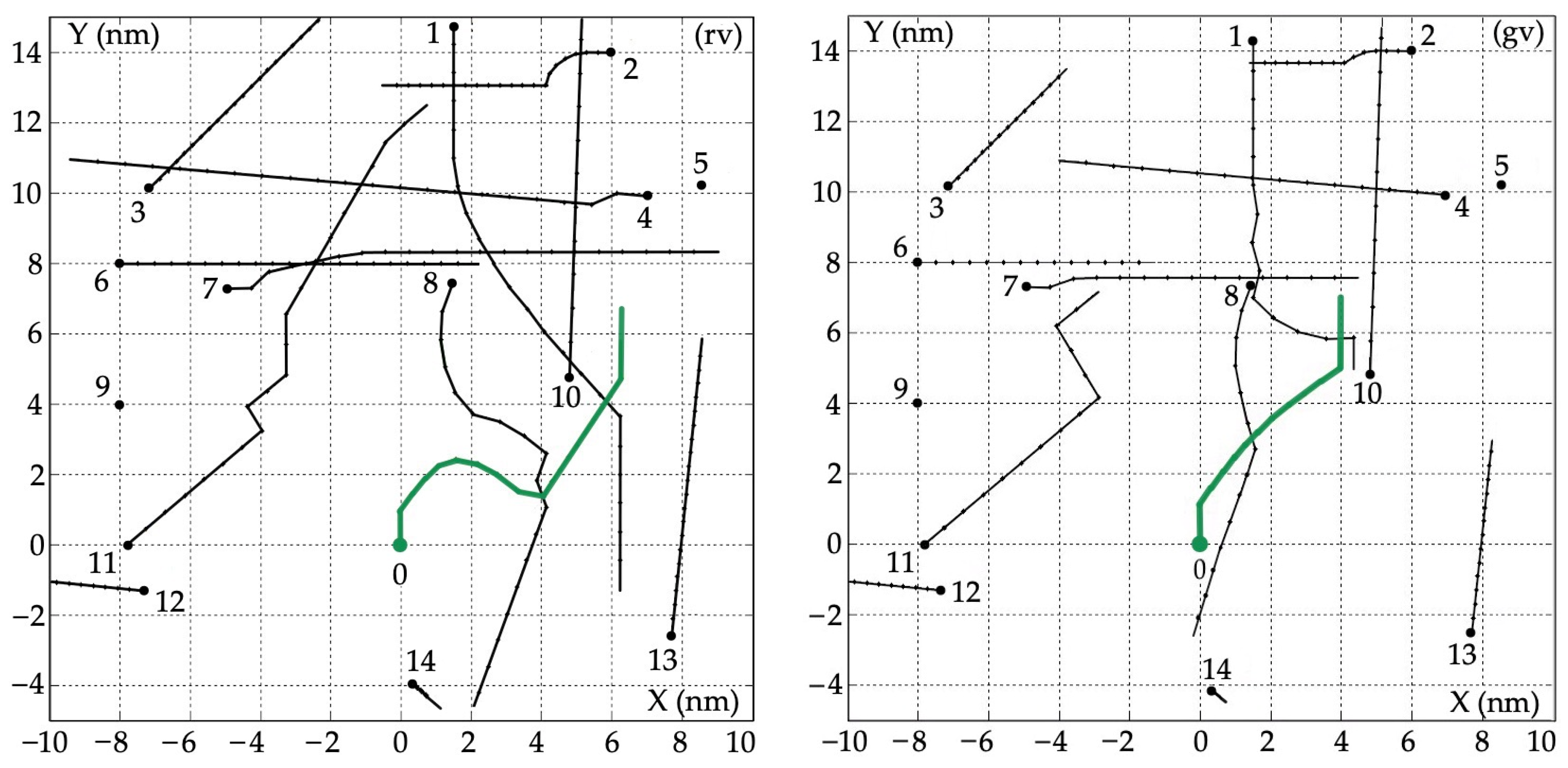
Figure 10.
Safety trajectories of Object 0 were determined using the t-oLP_c optimization algorithm in conditions of restricted (rv) and good (gv) visibility at sea.
Figure 10.
Safety trajectories of Object 0 were determined using the t-oLP_c optimization algorithm in conditions of restricted (rv) and good (gv) visibility at sea.

Figure 11.
Characteristics of the sensitivity of multi-objective optimization algorithms to changes in the sea state and degree of visibility at sea are reflected in the necessity of maintaining a safe passing distance of Ds between objects.
Figure 11.
Characteristics of the sensitivity of multi-objective optimization algorithms to changes in the sea state and degree of visibility at sea are reflected in the necessity of maintaining a safe passing distance of Ds between objects.


Table 1.
Values measured, using the ARPA anticollision system, of the state variables in the process of controlling the movement of Object 0 and fourteen passing objects.
Table 1.
Values measured, using the ARPA anticollision system, of the state variables in the process of controlling the movement of Object 0 and fourteen passing objects.
| Object j | Bearing Nj (deg) | Distance Dj (nm) | Speed Vj (kn) | Course ψj (deg) |
|---|---|---|---|---|
| 0 | - | - | 19.8 | 0 |
| 1 | 7 | 14.4 | 16.1 | 179 |
| 2 | 22 | 15.1 | 6.6 | 271 |
| 3 | 324 | 12.3 | 6.9 | 46 |
| 4 | 36 | 12.2 | 15.4 | 275 |
| 5 | 41 | 13.2 | 0 | 0 |
| 6 | 325 | 8.9 | 13.4 | 89 |
| 7 | 316 | 11.4 | 9.5 | 91 |
| 8 | 12 | 7.7 | 15.9 | 199 |
| 9 | 290 | 9.0 | 0 | 0 |
| 10 | 46 | 6.7 | 19.2 | 3 |
| 11 | 271 | 7.7 | 14.2 | 49 |
| 12 | 261 | 7.6 | 6.8 | 274 |
| 13 | 109 | 8.3 | 8.0 | 7 |
| 14 | 176 | 4.1 | 0.8 | 129 |
Table 2.
Values for the final deviation of the optimal safety trajectory of Object 0 from the initial trajectory.
Table 2.
Values for the final deviation of the optimal safety trajectory of Object 0 from the initial trajectory.
| Algorithm | s-oLP | b-oLP_nc | b-oLP_c | t-oLP_nc | t-oLP_c | |
|---|---|---|---|---|---|---|
| Deviation e (nm) | Restricted Visibility | 3.8 | 6.7 | 5.5 | 6.2 | 3.0 |
| Good Visibility | 2.0 | 3.6 | 3.0 | 4.0 | 2.8 | |
Disclaimer/Publisher’s Note: The statements, opinions and data contained in all publications are solely those of the individual author(s) and contributor(s) and not of MDPI and/or the editor(s). MDPI and/or the editor(s) disclaim responsibility for any injury to people or property resulting from any ideas, methods, instructions or products referred to in the content. |
© 2023 by the author. Licensee MDPI, Basel, Switzerland. This article is an open access article distributed under the terms and conditions of the Creative Commons Attribution (CC BY) license (https://creativecommons.org/licenses/by/4.0/).
Share and Cite
MDPI and ACS Style
Lisowski, J. Comparison of Multi-Object Control Methods Using Multi-Objective Optimization. Electronics 2023, 12, 4198. https://doi.org/10.3390/electronics12204198
AMA Style
Lisowski J. Comparison of Multi-Object Control Methods Using Multi-Objective Optimization. Electronics. 2023; 12(20):4198. https://doi.org/10.3390/electronics12204198
Chicago/Turabian StyleLisowski, Józef. 2023. "Comparison of Multi-Object Control Methods Using Multi-Objective Optimization" Electronics 12, no. 20: 4198. https://doi.org/10.3390/electronics12204198
Note that from the first issue of 2016, this journal uses article numbers instead of page numbers. See further details here.