Abstract
In this paper, we propose an innovative channel-sensitive autoencoder (CSAE)-aided end-to-end deep learning (E2EDL) technique for joint geometric probabilistic shaping. The pretrained conditional generative adversarial network (CGAN) is introduced in the CSAE which performs differentiable substitution of the optical fiber channel model under variable input optical power (IOP) levels. This enables the CSAE-aided E2EDL to design optimal joint geometric probabilistic shaping schemes for optical fiber communication systems at varying IOPs. The results of the proposed CSAE-aided E2EDL technique show that for a dual-polarization 64-Gbaud signal with a transmission distance of 5 × 80 km, when the modulation format is a 64-quadrature amplitude modulation (QAM) or a 128-QAM, the maximum generalized mutual information (GMI) level learned via CSAE-aided E2EDL is 5.9826 or 6.8384 bits/symbol under varying IOPs, respectively. In addition, the pretrained CGAN, as a substitution for optical fiber transmission model, accurately characterizes the distortion of signals with different IOPs, with an average bit error ratio (BER) difference of only 1.83%, an average mean square error (MSE) of 0.0041 and an average K-L divergence of 0.0046. In summary, this paper delivers new insights into the application of E2EDL and demonstrates the feasibility of joint geometric probabilistic shaping-based E2EDL for fiber optic communication systems with varying IOPs.
1. Introduction
Fiber optic communication systems have been extensively used in international internet communications and other areas and are some of the main technological backbones of information technology [1,2,3]. In recent years, deep learning neural networks (DLNNs) have been widely applied to enhance the transmission performance achieved in various aspects of optical fiber communication systems [4,5], which mainly consist of three components: a transmitter, channels and a receiver. At the transmitter, neural networks (NNs) can be used for constellation shaping (CS), which includes geometric shaping (GS) [6] and probabilistic shaping (PS) [7], to promote transmission flexibility. In terms of transmission channels, NNs exhibit strong channel fitting abilities, providing rapid channel simulation [8,9,10,11]. At the receiver, NNs are widely applied for nonlinear equalization and modulation format identification to compensate for signal distortion [12,13,14].
However, separately optimizing different blocks of a communication system does not always yield the optimal transmission performance. End-to-end deep learning (E2EDL), as a derivable neural network structure, is feasible to globally optimize the objective. The utilization of E2EDL allows optimization of the communication system as a whole with better global adaptability to improve the resulting transmission performance [15,16,17].
Many researchers have proposed several excellent network structures for E2EDL-based optical fiber communication system [18,19,20,21,22,23,24,25]. In 2018, Li et al. utilized an autoencoder to achieve GS of nonlinear phase noise channel [23]. In 2020, Cammerer et al. provided optimal GS results for symbol-wise and bit-wise autoencoder under an additive white Gaussian noise (AWGN) channel [20]. In order to achieve a differentiable autoencoder, these studies employed approximate channel models that make it difficult to consider the effects of chromatic dispersion (CD), polarization mode dispersion, and hardware impairments including those caused by splitters/couplers [26,27]. In 2022, Niu et al. implemented GS-based optical fiber E2EDL using an autoencoder with an enhanced Gaussian noise channel, which requires an additional NN to implement the gradient backpropagation process of the channel [18]. Nevertheless, most E2EDL schemes are only applied to GS, instead of joint probabilistic geometric shaping, for optical fiber transmission [18,19,20,21,22,23,24]. In 2022, Vahid et al. proposed an E2EDL-based joint geometric probabilistic shaping scheme under an AWGN channel [25], while this E2EDL is unable to characterize the variable signal impairment levels corresponding to different constellation points under different input optical powers (IOPs). There is a paucity of literature on E2EDL methods supporting combined fiber channel modeling with joint PS and GS under varying IOPs.
Against the above backdrop, in this paper, we present a channel-sensitive autoencoder (CSAE)-aided E2EDL technique for joint geometric probabilistic shaping, in which a pretrained conditional generative adversarial network (CGAN) is embedded to model optical fiber communication systems with varying IOPs. This technique can be used in optical fiber communication systems to optimize transmitter. Our contributions include the employment of a more accurate differentiable channel model that allows the simulation of different IOPs signals using only one NN. We also extend the joint optimization range of the autoencoder to include constellation position, probability, and IOP, for which we propose a power calibration scheme. The results show that for both 64-quadrature amplitude modulation (QAM) and 128-QAM, the CSAE-aided E2EDL technique learns the optimal IOP and constellation shaping scheme to achieve the maximum generalized mutual information (GMI).
The rest of this article is organized as follows. Section 2.1 describes the method of modeling E2E differentiable fiber transmission channel with variable IOPs using CGAN. Section 2.2 describes the structure of the CSAE and design of the power calibration method. Section 3 presents results and analysis involving the CGAN and CSAE. Finally, we provide a summary in Section 4.
2. CSAE-Aided End-to-End Deep Learning Scheme and Theory
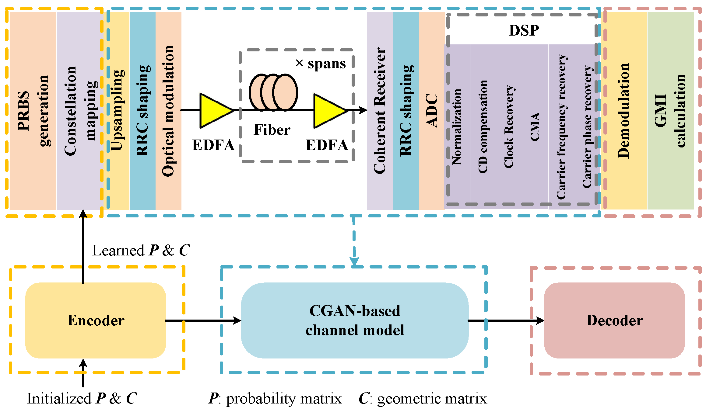
Figure 1 shows the schematic of the E2EDL strategy based on CSAE for the optical fiber communication system. In the actual optical fiber communication system, at the transmitter, the generated pseudorandom binary sequence (PRBS) performs constellation mapping, upsampling and root-raised cosine (RRC) shaping, followed by dual-polarization optical modulation. The channel employs a standard single-mode fiber, and the erbium-doped fiber amplifier (EDFA) is utilized to amplify the transmitting signal. The signal is obtained through a coherent receiver followed by a matched RRC filter, an analog-to-digital conversion (ADC) and a digital signal processing (DSP) module. As shown in Figure 1, in the CSAE-aided E2EDL scheme, the whole optical fiber communication system is mainly implemented as an encoder network, a decoder network and the CGAN-based differentiable channel network. The encoder outputs the learned optimal constellation map, including the probability and constellation coordinates of each constellation point. The CGAN-based differentiable channel network is introduced to substitute the circled part of optical fiber communication system. The decoder is used to convert the received signals into the bit sequences in a log-likelihood form.
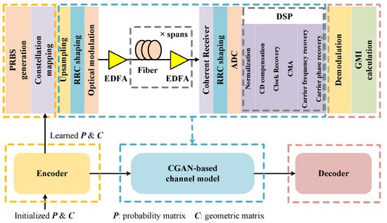
Figure 1.
The schematic of the E2EDL strategy based on CSAE for the optical fiber communication system (PRBS: pseudorandom binary sequence; RRC: root-raised cosine; EDFA: erbium-doped fiber amplifier; ADC: analog-to-digital conversion; CMA: constant modulus algorithm).
2.1. CGAN-Based Differentiable Optical Fiber Transmission Model
A major challenge regarding the E2E optimization of a probability shaping signal is that the entropy of the signal changes during the optimization process, which means that the IOP also changes; this requires the NN to simulate the channel environment under various IOPs. To enable the CSAE to support a continuously changing IOP during iterative training, we design a CGAN-based optical fiber transmission model for substituting a non-differentiable optical fiber channel. This structure supports adding corresponding channel impairment to the signal with a varying IOP level.
Figure 2 shows the structure of CGAN, which consists of a generator and a discriminator. The generator is responsible for substituting the circled part of the optical fiber communication system, which is shown is Figure 1. The discriminators are used to determine the credibility of the generator. Circles in the generator and discriminator represent NN nodes.
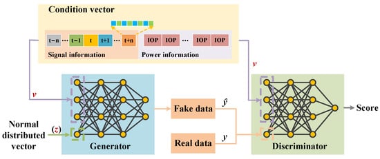
Figure 2.
The Schematic diagram of CGAN.
The condition vector v and a group of normally distributed vectors z constitute the input of the generator. As shown in Figure 2, the condition vector is composed of signal information and power information of IOP. Due to the influence of pulse broadening caused by dispersion, the condition vector should not only consider the signal at the current moment t, but also introduce the signal at n moments before and after the current moment. The signal at each moment contains a four-time upsampled IQ amplitude for a total of eight features. Therefore, the signal characteristic dimensionality is 8 × (2n + 1).
To enable the generator to learn the signal damage induced under different powers, it is necessary to carefully design the IOP characteristic dimensions. When there are fewer dimensions of IOP features, the IOP characteristics are easy to average by batch normalization and difficult to learn with an NN. In contrast, when the IOP characteristic dimensionality is too large, the signal characteristic is difficult to learn. We find that when the IOP dimensionality is the same as the signal dimensionality, the generator can effectively generate channel damage under various powers. By integrating the signal information and power information of IOP, it can be concluded that the characteristic dimensionality of the condition vector is 2 × 8 × (2n + 1). To make the CGAN more robust, the generator also introduces a set of 10-dimensional standard normal distribution vectors z as noise. Different input noises enable the generator to generate diverse data. The fake data generated by the generator and the real data y are alternately input into the discriminator. At the same time, the condition vector v is also input into the discriminator.
The evaluation functions used to update the generator and discriminator can be represented as
where represents the output score of the real data y corresponding to the condition vector v through the discriminator, and denotes the output score of the fake data passing the discriminator.
During the iterative process, the discriminator and the generator are alternately trained. The discriminator is trained to simultaneously minimize and maximize . When tends to ln, the CGAN converges; that is, the Nash equilibrium is realized [9].
Significantly, to ensure that the CGAN can learn the channel noise under different IOPs, the training data samples should come from different IOPs to the greatest extent possible. When the training process of the CGAN is completed, embedding the well-trained generator into the CSAE enables the CSAE to perform E2EDL for optical fiber communication systems. One advantage of the proposed CGAN-based neural network is differentiable and the gradient information is retained. Therefore, the encoder of the CSAE can be directly updated by gradient backpropagation through the CGAN-based differentiable neural network.
2.2. Principles of the Proposed CSAE
This section demonstrates the principles of the CSAE. The CSAE can generate signals under varying IOP and reconstruct them into bit sequences in a log-likelihood form, continuously optimizing the modulation format through E2EDL by maximizing the GMI.
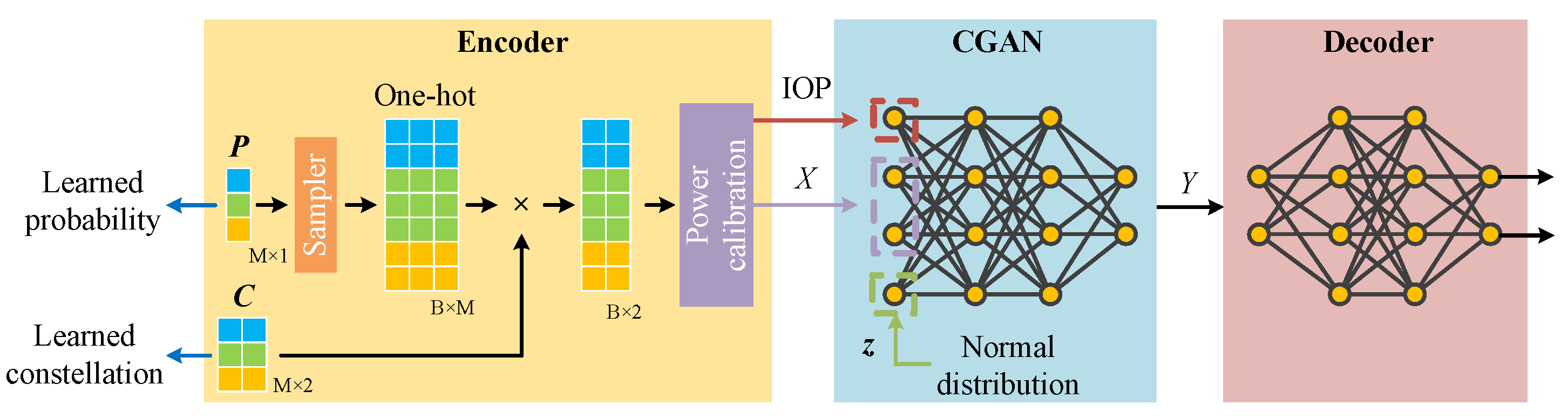
Figure 3 shows the structure of the CSAE, which is composed of an encoder network, a decoder network and the pretrained differentiable CGAN-based channel model. The arrows represent the direction of data flow. The encoder network stores the probability and constellation coordinates of each constellation point in the form of weights for the single fully connected layer. For the M-QAM modulation format, the probability information of the constellation is stored in a weight matrix of size M × 1, and the geometric information of the constellations is stored in a weight matrix of size M × 2.
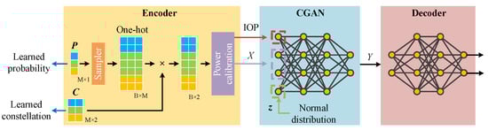
Figure 3.
The Schematic diagram of CSAE.
The sampler in Figure 3 is used to sample the probability matrix and generate the training symbols with batch size B, which stored as a one-hot coding matrix of size B × M [25]. Due to the size limitation of B, the consistency of the probability matrix and the training symbols refers to [28]. Then, the one-hot coding matrix is disordered [25] and multiplied by geometric matrix to obtain the transmitted signals of size B × 2.
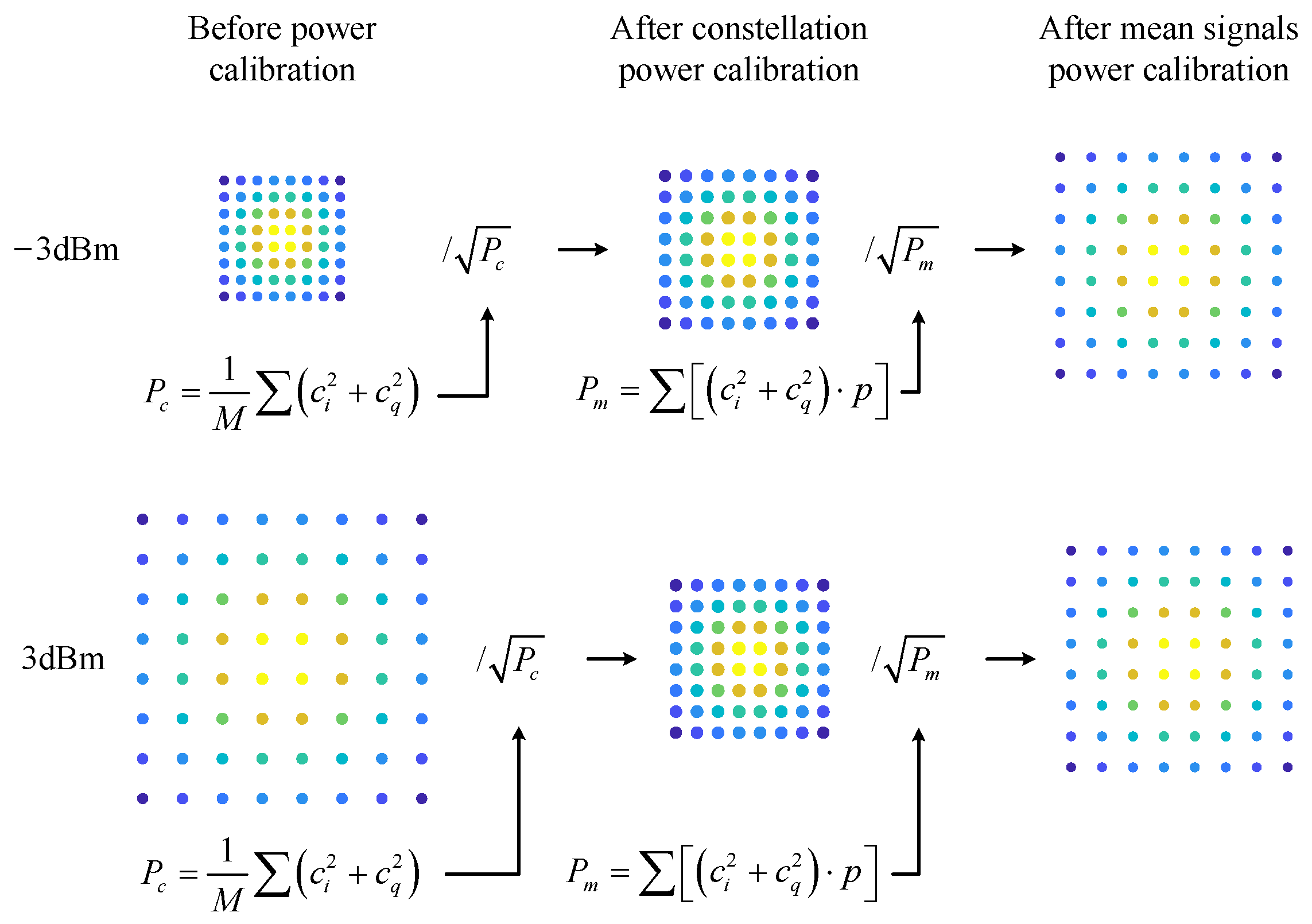
Note that during the training of CGAN in Section 2.1, the signal input into the CGAN is normalized. Since different IOPs lead to a change in the value of the geometric matrix , the transmitted signal amplitude is different. Moreover, the signal amplitude with different probability matrix also changes in order to keep the transmit power constant. In order to correctly match the encoder and CGAN, we propose a power calibration method and realize the transmitted signal normalization as shown in Figure 4. The size of the constellations represents their coordinates, and the color of the points represents their probabilities, with lighter colors indicating higher probabilities. The proposed power calibration process is divided into two steps: constellation power calibration and mean signal power calibration. Firstly, the transmitted signals are divided by . Here, is defined as the constellation power, which is expressed as
where I and Q are elements in geometric matrix , which correspond to the in-phase and quadrature of the constellation, respectively. Note that is logged and used to later generate the condition vector for CGAN. Secondly, the above signals are then divided by , and is called the mean signal power, which is defined as
where p is the element in probability matrix , which corresponds to the probability of the corresponding constellation point.
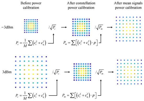
Figure 4.
Diagram of the power calibration process.
The constellation with different IOP values is distributed differently. After power calibration, the constellations are normalized and the normalized signal X is fed into the pretrained CGAN to simulate the transmission impairment under varying IOPs. Note that the normalized signal X is sampled through a sliding window to obtain the signal information of the condition vector v in Figure 2. The power information of condition vector v is the IOP, which is logged in . During CSAE training, the weights of the pretrained CGAN are fixed to accurately model the damaged signals.
The decoder in Figure 3 is composed of three fully connected layers with a trainable parameter , which is used to convert IQ signals into binary bit sequences in a log-likelihood form. The input layer is composed of two features, which come from the output of the CGAN. The hidden layer section is a two-layer 128-dimensional fully connected NN, and the activation function is a Leaky ReLU. The dimensionality of the output layer is , and the sigmoid function is used to distribute the output range in [0,1].
Depending on the requirements, the CSAE can work in two different modes, fixed IOP and adaptive IOP.
2.2.1. Fixed IOP
In the fixed IOP mode, the power information in the condition vector of the CGAN is set as the given IOP. The CSAE-aided E2EDL scheme can be performed and output the corresponding learned geometric matrix and probability matrix at the specified IOP. In this mode, the constellation power is only used for normalization in the power calibration. Therefore, it needs to be detached from gradient back propagation.
2.2.2. Adaptive IOP
In the actual optical fiber communication system, a suitable IOP value would achieve a optimal GMI. In such a context, the adaptive IOP mode is initially designed. In the adaptive IOP mode, the power information in the condition vector of the CGAN is set as the the constellation power . During the gradient back propagation process of CSAE, the loss function updates through . After the training process of CSAE is completed, the corresponding is the optimal IOP. And the corresponding learned geometric matrix and probability matrix at the optimal IOP would be output from the encoder of CSAE.
In the encoder, benefitting from the power calibration, the isometric scaling geometric matrix has no effect on CGAN; hence, we innovatively use this property to implement E2EDL for a varying IOP range.
Considering that GMI reflects the maximum achievable information rate for a bit-metric decoding system [20], we utilize the negative value of GMI as a loss function of the CSAE, which is expressed as Equation (5).
where is the entropy of the constellation; is the kth bit of the binary sequence corresponding to each element in ; is the edge probability of ; represents the posterior probability of when is known; and describes the probability that the decoder can determine = 1 given that , and are known, which can be directly derived by the decoder. The CSAE optimizes parameters and during the process of maximizing GMI. The optimization parameter is the process of PS, and the optimization parameter is the process of GS.
3. Results and Analysis
3.1. Accuracy Analysis of CGAN-Based Differentiable Optical Fiber Transmission Model
In the simulation, we keep the nonlinear coefficient of the optical fiber communication system unchanged and control the nonlinear effect by adjusting the IOP. The system structure is shown in Figure 1. Parameters are referenced to G.652 fiber. The fiber attenuation used in the system is 0.2 dB/km. The dispersion and dispersion slope are 16 ps/nm/km and 0.08 ps/nm/km, respectively. The polarization mode dispersion coefficient between two polarization states is 0.1 ps/km. The effective area and (which impacts the nonlinear effect) are 80 m and 2.6 × 10 m/W, respectively. As for EDFA, we set the noise figure to 3.8 dB and the noise bandwidth to 4 THz. The laser wavelength is 1550 nm, and the linewidth is 100 kHz. The frequency offset of the local oscillatory is 1MHz. The baud rate of the system is 64-Gbaud. The roll-off factor of the root raised cosine filter is set to 0.2. The number of fiber spans is set to five, and the IOP is set from −5 to 5 dBm. The detailed parameters of DSP are as follows: CD compensation is implemented by a frequency-based algorithm. The clock recovery is performed using Gardner’s algorithm. The constant modulus algorithm (CMA) equalizer convergence factor is , the number of taps is 17 and the RRC response with a roll-off factor of 0.2 is used as the initial value of the taps. Carrier frequency recovery (CFR) is implemented based on the fourth power. Carrier phase recovery (CPR) is performed using a pilot-aided algorithm that is insensitive to PS.
The parameters of the CGAN are shown in Table 1.

Table 1.
Parameters of the CGAN.
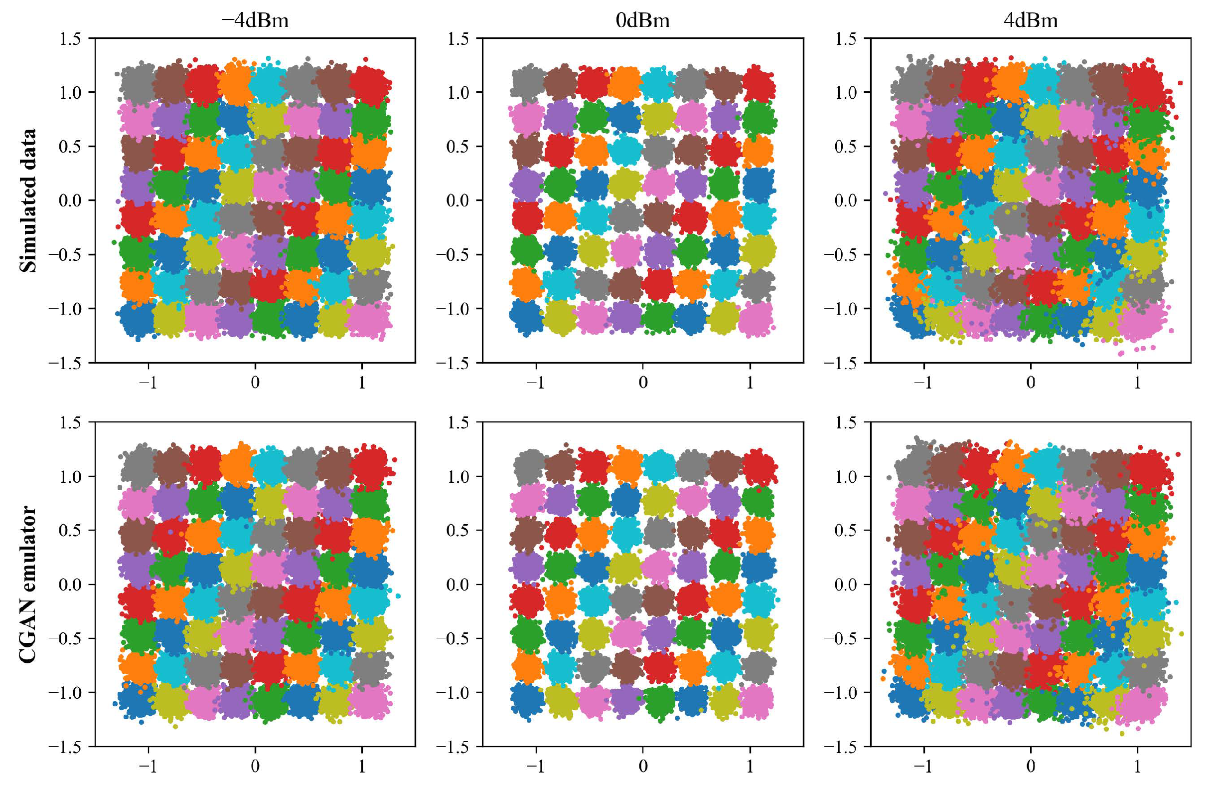
Figure 5 shows the modeling accuracies achieved at different IOPs for a transmission distance of 5 × 80 km. To clearly show the results, we carry out downsampling processing. Adjacent constellation points are distinguished by different colors. For an optical fiber communication system, the received signal is distorted, and the damage becomes more severe as the IOP increases. Comparing the output constellations of the simulation data and the differentiable CGAN emulator, it can be seen that the spatial distributions of the clusters in the two groups of results are highly consistent, which shows that the CGAN has successfully learned the optical fiber transmission damage and proves the effectiveness of the CGAN differentiable model scheme.
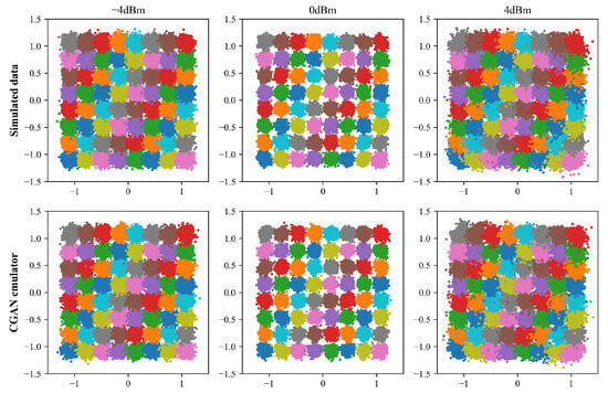
Figure 5.
Constellations of the simulated data and the CGAN emulator output at −4, 0, and 4 dBm IOPs.
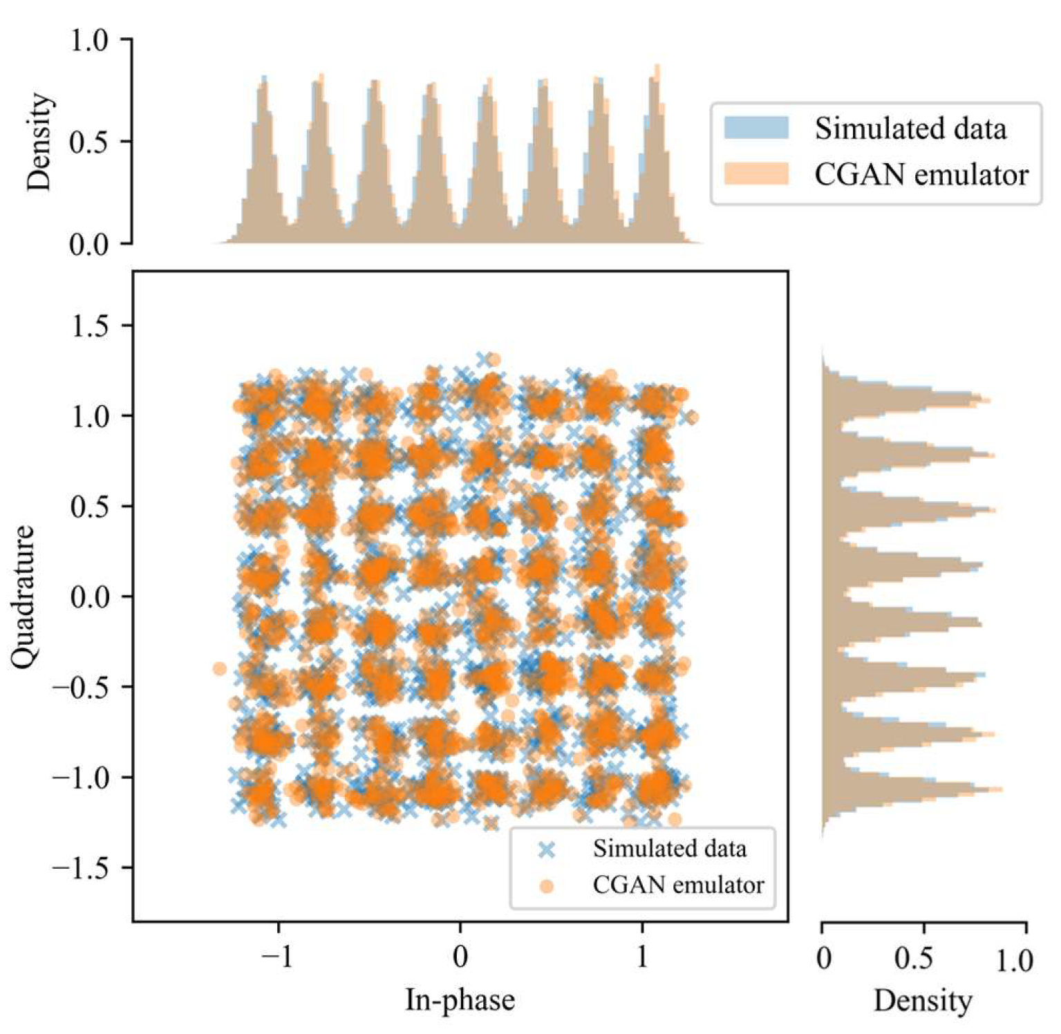
Figure 6 shows the constellation of the simulated data and the CGAN emulator output when the channel parameters are set to 5 × 80 km and 4 dBm and gives their corresponding density distributions of in-phase and quadrature parts. The difference in the distribution of the simulated data and the CGAN emulator is measured by the K-L divergence, which is only 0.0046 on average. The K-L divergence for two discrete distributions and is , where b is the data length. Figure 6 illustrates that the CGAN emulator produces almost the same data distribution as the simulation data.

Figure 6.
Data distribution and kernel density map for the simulated data and the CGAN emulator.
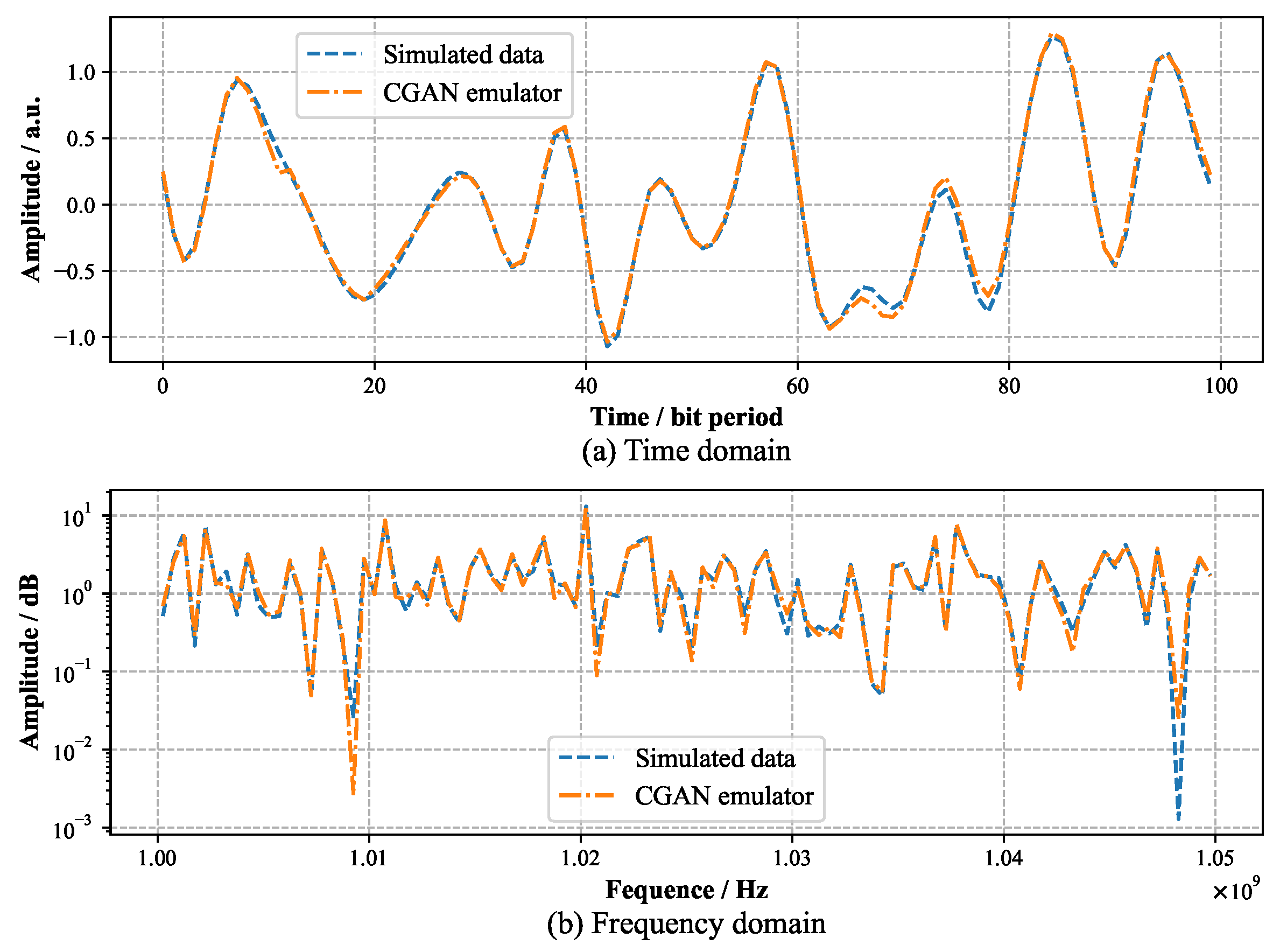
To intuitively prove the accuracy of the CGAN-based optical fiber transmission model, we compare the time domain and frequency domain waveforms of the simulation data and the CGAN output when the IOP is set to 4 dBm as shown in Figure 7. Notably, the outputs of the simulation data and the CGAN emulator in Figure 7a exhibit high similarity, but they are not exactly the same, with a mean square error (MSE) of 0.0041. MSE is expressed as , where b is the data length.
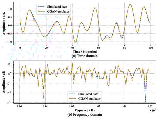
Figure 7.
Comparison between the time domain and frequency domain waveforms of the simulated data and the CGAN emulator.
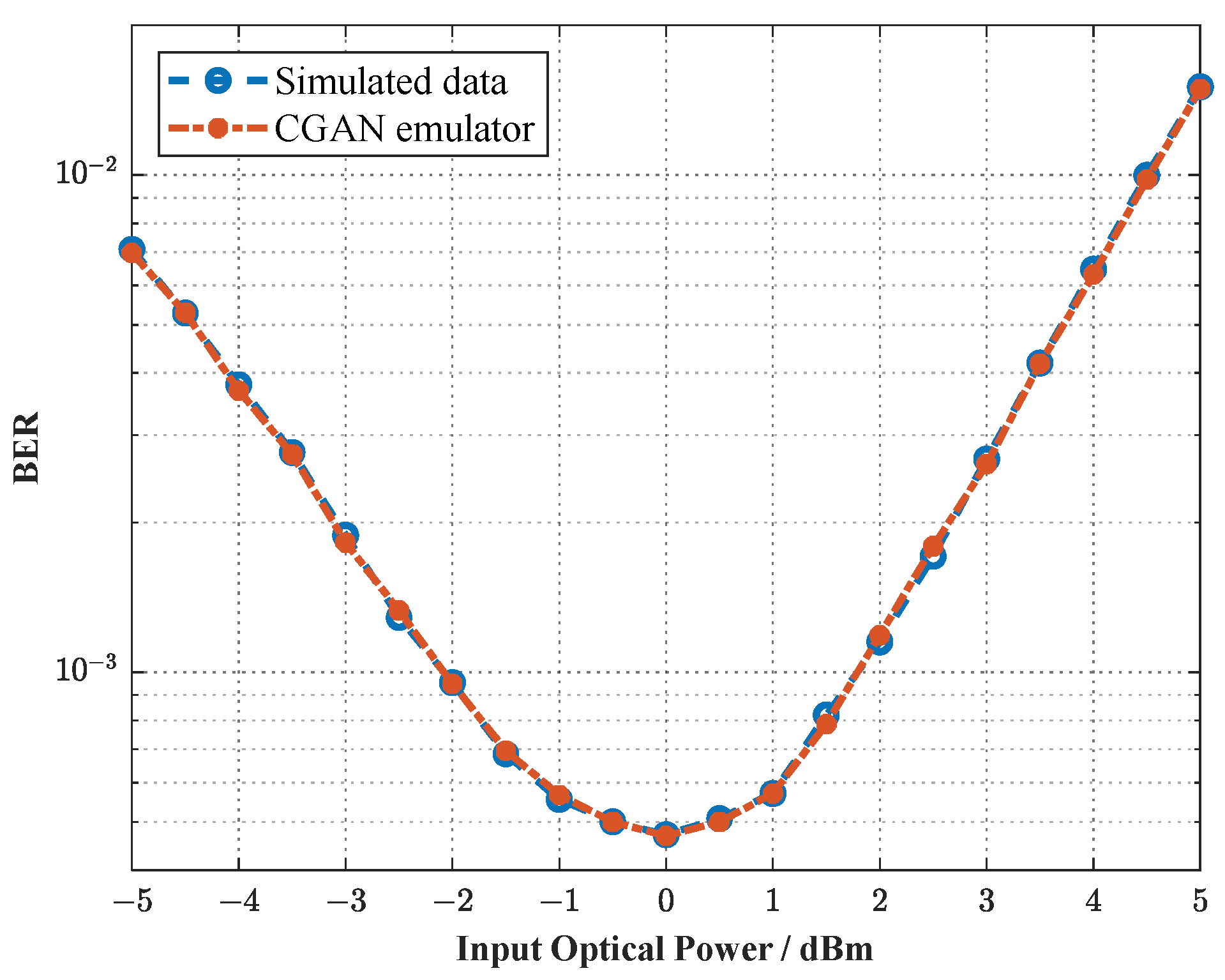
Figure 8 shows the bit error ratio (BER) comparison between the optical fiber communication system and the CGAN-aided reconstruction approach under different IOPs with the same demodulator. The BER performances of both approaches are highly identical, with an average error of only 1.83%, indicating that the CGAN has sufficient capacity to replace the optical fiber communication system. Figure 5, Figure 6, Figure 7 and Figure 8 prove that the established CGAN has strong robustness to channel reconstruction and truly reflects the channel situation.
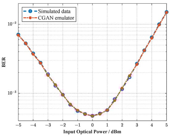
Figure 8.
BER comparison after utilizing the optical fiber transmission system and CGAN under different IOPs.
3.2. Performance Validation of the CSAE
In this section, we use the CSAE to perform E2EDL on the optical fiber communication system in Section 3.1. The parameters of the CSAE are shown in Table 2. Then, we show the optimization results produced by the CSAE working in the adaptive IOP mode and compare them with the results obtained when working in the fixed IOP mode, as shown below.
Table 2.
Parameters of the CSAE.
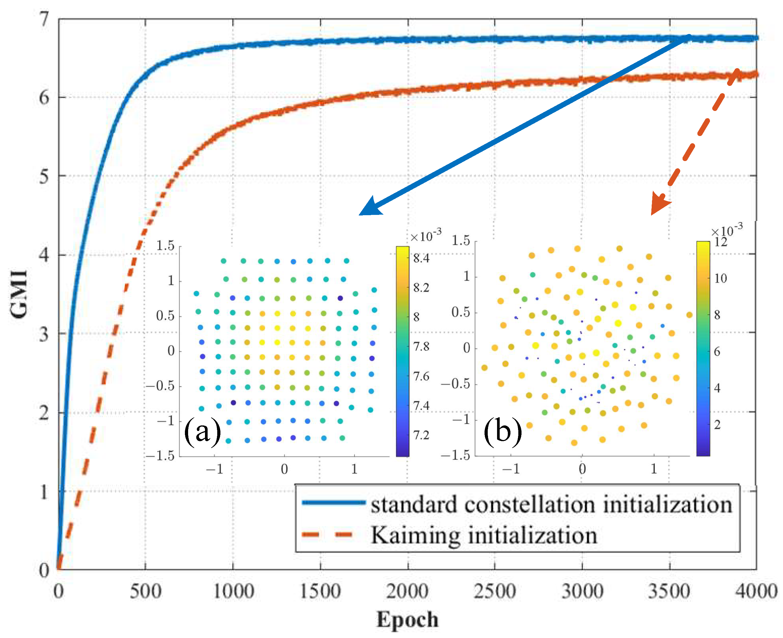
In order for appropriate initialized parameters, including and , to effectively avoid the CSAE falling into a local optimum while speeding up training, appropriate initial conditions need to be set. We find that the convergence of the CSAE is better when the weight matrix is initialized with the standard constellation instead of the common Kaiming initialization [29]. As shown in Figure 9, the CSAE with Kaiming initialization has difficulty converging to the optimum, while using the standard constellation initialization allows rapid convergence of the CSAE. Furthermore, the initial values of the weight matrix are all set to , that is, the initial constellation is evenly distributed.
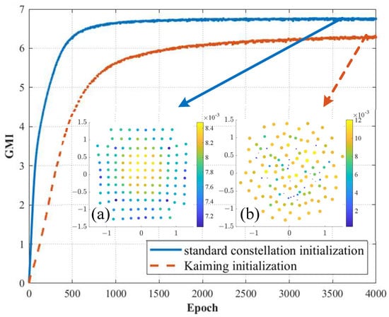
Figure 9.
GMI achieved in each epoch using different initializations when IOP is 2 dBm. (a) Standard constellation initialization; (b) Kaiming initialization.
3.2.1. Fixed IOP Mode
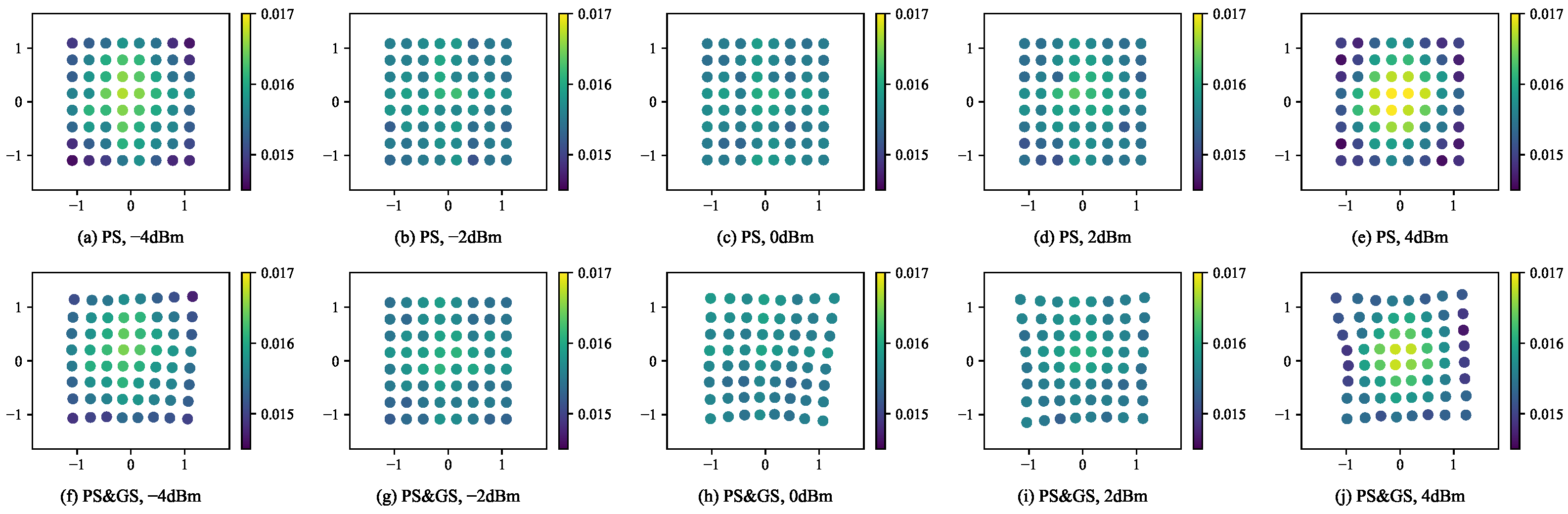
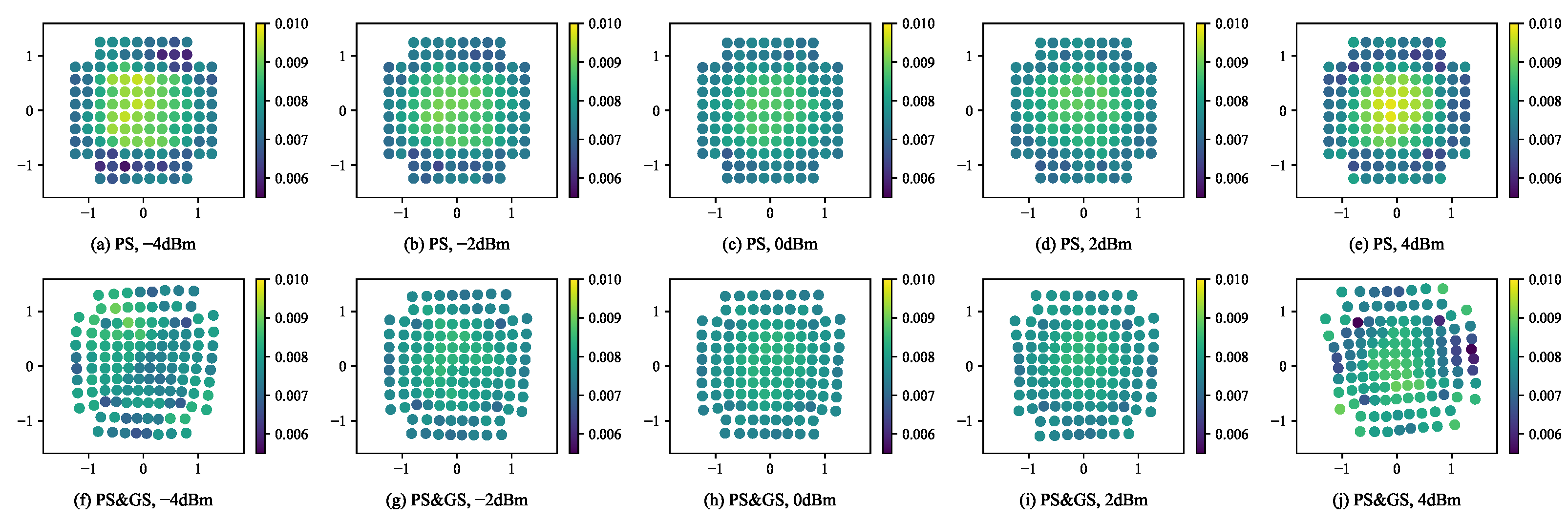
In Figure 10 and Figure 11, the E2EDL results obtained when using only PS and using joint PS and GS with different IOPs are shown. The constellations derived from the two methods are more uniform and have larger entropy when the IOP is 0 dBm. As the IOP increases or decreases, the CSAE uses a more pronounced PS scheme to make the GMI of the E2EDL as large as possible. Since the position of the constellation in the PS-only scheme is fixed, the entropy needs to be sacrificed to achieve a higher degree of shaping to maximize the GMI. In contrast, the constellation with the joint PS and GS scheme can adopt a larger entropy to obtain a higher upper boundary of the GMI. Due to the self-phase modulation (SPM) of the fiber, the phase noise of the signal increases when the IOP is too large. Considering only the case of SPM, the nonlinear Schrödinger equation can be written as , where A is the amplitude of the signal, z is the fiber transmission direction, and is the nonlinear coefficient. The GS scheme designs the distance between the constellation points with high power farther away from each other to reduce the effect of SPM.
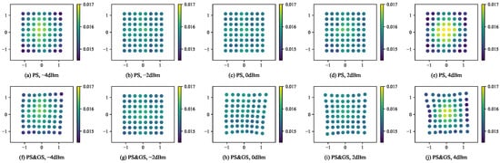
Figure 10.
64-QAM constellations designed by the CSAE under different IOPs (above: PS; below: PS and GS).
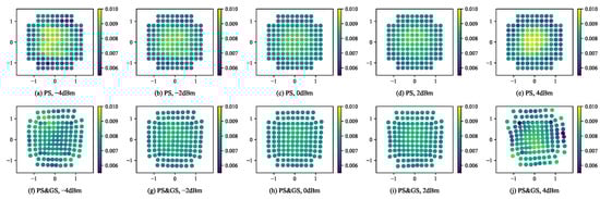
Figure 11.
128-QAM constellations designed by the CSAE under different IOPs (above: PS; below: PS and GS).
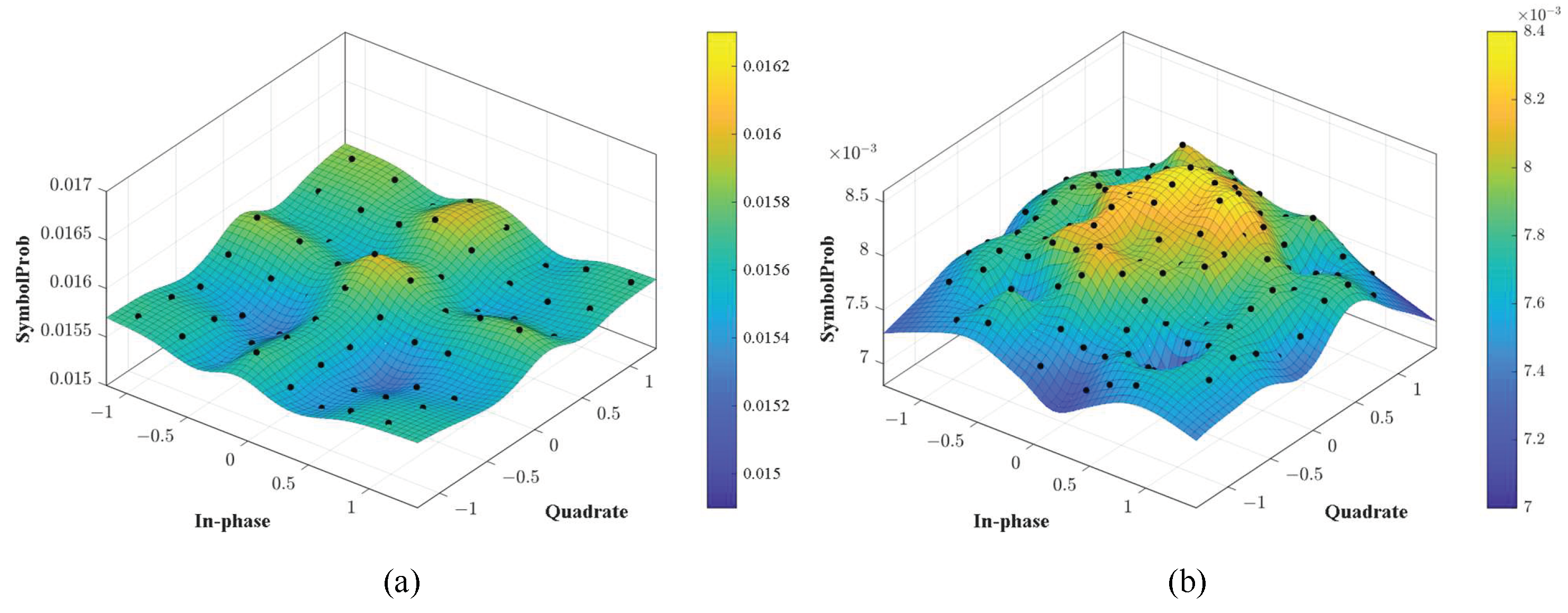
Figure 12 fits the constellation points and probability using only PS as well as joint PS and GS into a distribution when IOP is 5 dBm and compares it with the Maxwell–Boltzmann (M-B) distribution with the same entropy as using PS, which is the optimal distribution in the AWGN channel [30]. The fitting process is performed by thin plate spline interpolation. Using only PS produces a similar degree of shaping as using the M-B distribution, except that the probabilities are higher at high power constellation points. Using joint GS and PS results in less pronounced shaping than when using the M-B distribution, and therefore produces higher entropy as well as a higher upper limit of GMI.
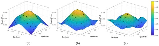
Figure 12.
Comparison of the probability distributions produced by different schemes. (a) Maxwell–Boltzmann distribution; (b) PS only; (c) joint PS and GS.
3.2.2. Adaptive IOP Mode
E2EDL results in optimal joint geometric probability shaping schemes for 64-QAM and 128-QAM as shown in Figure 13. The optimal IOP for 64-QAM is 0.4988 dBm, and the maximum GMI is 5.9826 bits/symbol. In this case, the channel environment is better, so the distribution is closer to uniform, which maximizes the entropy. The optimal 128-QAM transmission power is 0.6559 dBm, and the maximum GMI is 6.8384. As the modulation order increases, the degree of probabilistic shaping becomes more pronounced to maximize the GMI. The distribution derived from E2EDL differs from the M-B distribution that is widely used in AWGN channels. The constellation points with low power obtain higher probabilities, as do the constellation points in the surrounding area, which are less likely to be misjudged.

Figure 13.
Optimal shaping schemes. (a) Distribution map obtained by interpolation for 64-QAM; (b) distribution map obtained by interpolation for 128-QAM.
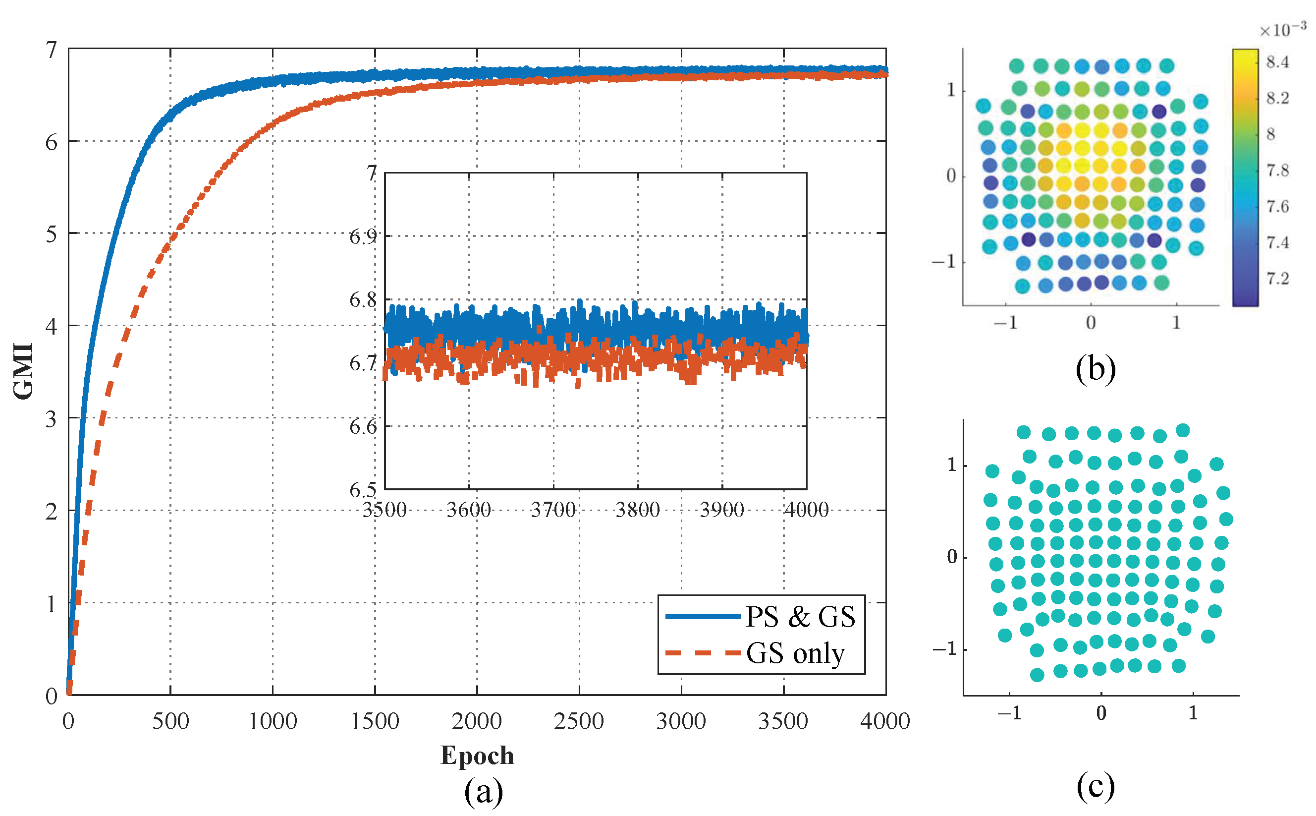
To illustrate the limitations of using only GS, we compare the GMI achievement of the GS-only scheme with the joint PS and GS scheme, as shown in Figure 14. The results show that the joint PS and GS scheme achieves a higher GMI than the GS-only scheme.
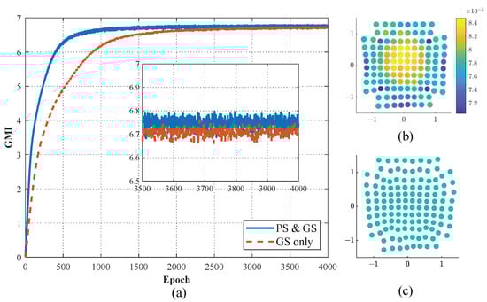
Figure 14.
(a) GMI achieved for E2EDL with different optimization modes in each epoch when IOP is 2 dBm; (b) PS and GS; (c) GS only.
3.2.3. Comparison between the Fixed IOP Mode and the Adaptive IOP Mode
To quantitatively show the effectiveness of the CSAE for optical fiber communication systems in the adptive IOP mode, we calculate and compare the GMI performance of the transmission system with the constellations designed by the CSAE in the fixed mode and the adaptive IOP mode, respectively.
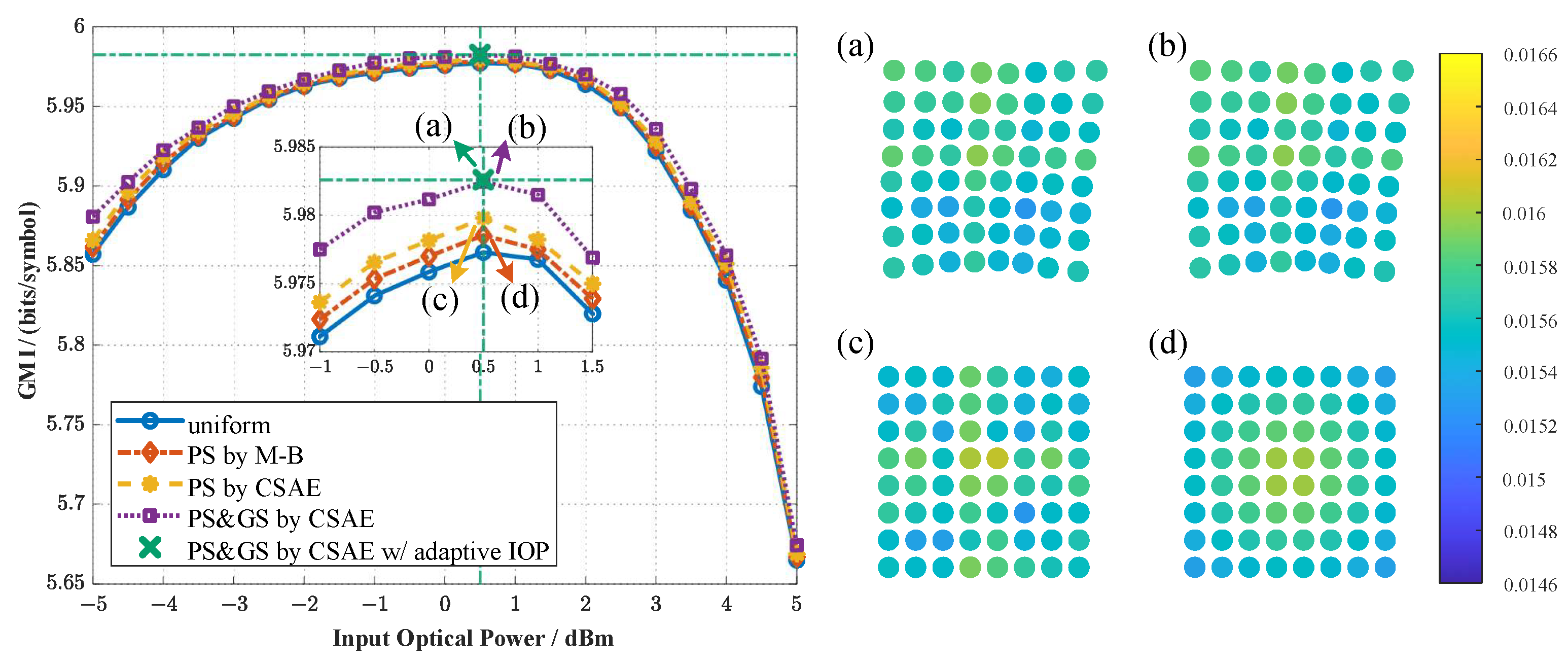
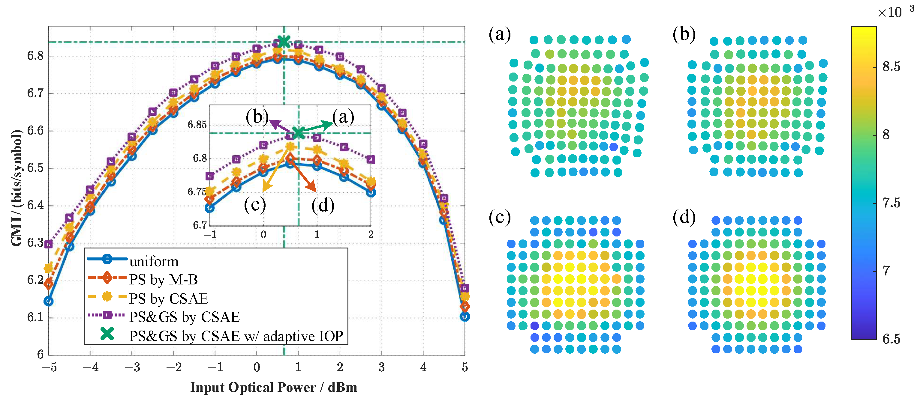
Figure 15 and Figure 16 show the GMI performance of the CSAE with different operating modes at different IOPs. Under the same channel environment, we choose the uniform signal as well as the PS signal with M-B distribution as a baseline. Note that the entropy of the PS signal with M-B distribution is the same as that of the CSAE with PS only. We compare the performance of CSAE with PS only and with PS and GS under different IOPs, and also present the performance of CSAE with the PS and GS scheme using adaptive IOP. Overall, the PS scheme learned by CSAE achieves a higher GMI than the PS scheme with an M-B distribution over the entire IOP range. For the PS scheme and the PS and GS scheme learned by CSAE, the latter obtains a higher GMI. For the 64-QAM CSAE scheme which is shown in Figure 15, the maximum GMI of 5.9826 bits/symbol at the optimal IOP (0.4988 dBm) (marked with the fork) is obtained in the adaptive IOP mode and the corresponding constellation with joint geometric probability shaping is shown in Figure 15a. For the 128-QAM CSAE scheme in Figure 16, the maximum GMI of 6.8384 bits/symbol at the optimal IOP (0.6559 dBm) (marked with the fork) is obtained from the proposed CSAE scheme and the corresponding constellation with joint geometric probability shaping is shown in Figure 16a. Finally, the GMI gains are calculated at the optimal IOP. For the joint PS and GS scheme, the CSAE in the adaptive IOP mode provides the maximum GMI, which is 0.0053 and 0.046 bits/symbol higher than those of the uniform modulation format for 64-QAM and 128-QAM, respectively, and which is 0.004 and 0.038 bits/symbol higher than those of the PS modulation format by the M-B distribution for 64-QAM and 128-QAM, respectively.
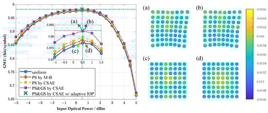
Figure 15.
GMI achieved for 64-QAM E2EDL under different IOPs. (a) PS and GS by CSAE w/adaptive IOP; (b) PS and GS by CSAE; (c) PS by CSAE; (d) PS by M-B.
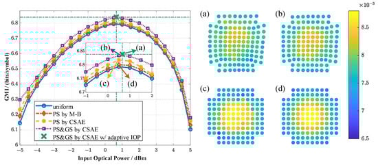
Figure 16.
GMI achieved for 128-QAM E2EDL under different IOPs. (a) PS and GS by CSAE w/adaptive IOP; (b) PS and GS by CSAE; (c) PS by CSAE; (d) PS by M-B.
This paper investigates E2EDL for optical fiber communication systems using a CSAE with an embedded CGAN, which effectively reflects the distributed characteristics of such a system and can model systems opearting under different IOPs using only a single network. The proposed CSAE shows the ability to optimize the joint probabilistic geometric shaping modulation format under varying IOPs. Benefiting from the CGAN’s differentiable model capabilities for optical fiber communication systems with different IOPs, the CSAE can provide both modulation schemes and IOPs suitable for these systems, further improving their transmission performance.
4. Conclusions
In this paper, we propose a CSAE for E2EDL for optical fiber communication systems. The proposed scheme supports joint geometric probability shaping at a fixed IOP as well as the joint optimization for the IOP and constellation shaping to obtain the maximum GMI for a communication system. To achieve E2E differentiability, we design a CGAN for differentiable substitution in optical communication systems. The results show that the BER evaluated with the CGAN-aided modeling approach is fitting to that of the real optical communication system, with an MSE of 0.0041 and a K-L divergence of 0.0046 between the two, thus proving the feasibility of this approach. In addition, we separately analyze the results of two CSAE operating modes. The E2EDL results for either a PS or joint PS and GS scheme can be obtained separately under each IOP using the fixed IOP mode. When the IOP is too high or too low, PS becomes more effective in maximizing the GMI, and the shaping effect is more pronounced when employing PS only than when utilizing joint PS and GS. A higher GMI can be achieved with an adaptive IOP than with a fixed IOP. For 64-QAM, the proposed CSAE-aided E2EDL shows that the obtained joint geometric probability shaping can result in a maximum system GMI of 5.9826 bits/symbol at 0.4988 dBm, with a GMI gain 0.004 bits/symbol compared to PS signals with the M-B distribution. For 128-QAM, the maximum GMI reaches 6.8384 bits/symbol at 0.6559 dBm, corresponding to a GMI gain of 0.038 bits/symbol compared to PS signals with the M-B distribution. The results demonstrate the feasibility of the proposed joint geometric probabilistic shaping-based E2EDL method for optical communication systems.
Author Contributions
Conceptualization, Y.L. and H.C.; methodology, Y.L., R.G. and Q.Z.; software, Y.L. and F.W.; validation, Y.L. and F.T.; formal analysis, Y.L., R.G. and H.Y.; investigation, Y.L. and H.C.; resources, Q.T. and L.R.; data curation, Y.W. and F.T.; writing—original draft preparation, Y.L. and H.C.; writing—review and editing, Y.L., H.C. and Q.Z.; visualization, H.C. and Y.W.; supervision, Q.Z. and X.X.; project administration, X.X.; funding acquisition, Q.Z. and H.C. All authors have read and agreed to the published version of the manuscript.
Funding
This work was funded in part by the National Key R&D Program of China from the Ministry of Science and Technology under Grant 2021YFB2800903, in part by the State Key Program of National Natural Science of China (Grant No. 61835002, 61935005, 62105026, 62105027, 62206018), the Funds for Creative Research Groups of China (Grant No. 62021005).
Data Availability Statement
Data underlying the results presented in this paper are not publicly available at this time but may be obtained from the authors upon reasonable request.
Conflicts of Interest
The authors declare no conflict of interest.
References
- Dong, Z.; Yu, J.; Chen, Y.; Li, F.; Xin, X. Symbol division multiplexing in optical fiber communication systems. Opt. Express 2022, 30, 14998–15007. [Google Scholar] [CrossRef]
- Chai, F.; Zhang, Q.; Yao, H.; Xin, X.; Gao, R.; Guizani, M. Joint Multi-task Offloading and Resource Allocation for Mobile Edge Computing Systems in Satellite IoT. IEEE Trans. Veh. Technol. 2023, 72, 7783–7795. [Google Scholar] [CrossRef]
- Ma, S.; Yao, H.; Mai, T.; Yang, J.; He, W.; Xue, K.; Guizani, M. Graph Convolutional Network Aided Virtual Network Embedding for Internet of Thing. IEEE Trans. Netw. Sci. Eng. 2023, 10, 265–274. [Google Scholar] [CrossRef]
- Cheng, Y.; Zhang, W.; Fu, S.; Tang, M.; Liu, D. Transfer learning simplified multi-task deep neural network for PDM-64QAM optical performance monitoring. Opt. Express 2020, 28, 7607–7617. [Google Scholar] [CrossRef] [PubMed]
- Wang, K.; Wang, C.; Zhang, J.; Chen, Y.; Yu, J. Mitigation of SOA-Induced Nonlinearity With the Aid of Deep Learning Neural Networks. J. Light. Technol. 2022, 40, 979–986. [Google Scholar] [CrossRef]
- Ait Aoudia, F.; Hoydis, J. Waveform Learning for Next-Generation Wireless Communication Systems. IEEE Trans. Commun. 2022, 70, 3804–3817. [Google Scholar] [CrossRef]
- Jing, Z.; Tian, Q.; Xin, X.; Wang, Y.; Guo, D.; Sheng, X.; Yu, C. Probabilistic shaping communication system aided by neural network distribution matcher in data center optical network. Microw. Opt. Technol. Lett. 2021, 63, 2274–2278. [Google Scholar] [CrossRef]
- Wang, D.; Song, Y.; Li, J.; Qin, J.; Yang, T.; Zhang, M.; Chen, X.; Boucouvalas, A.C. Data-driven Optical Fiber Channel Modeling: A Deep Learning Approach. J. Light. Technol. 2020, 38, 4730–4743. [Google Scholar] [CrossRef]
- Yang, H.; Niu, Z.; Xiao, S.; Fang, J.; Liu, Z.; Fainsin, D.; Yi, L. Fast and Accurate Optical Fiber Channel Modeling Using Generative Adversarial Network. J. Light. Technol. 2021, 39, 1322–1333. [Google Scholar] [CrossRef]
- Jiang, R.; Fu, Z.; Bao, Y.; Wang, H.; Ding, X.; Wang, Z. Data-Driven Method for Nonlinear Optical Fiber Channel Modeling Based on Deep Neural Network. IEEE Photonics J. 2022, 14, 1–8. [Google Scholar] [CrossRef]
- Ye, G.; Xiang, J.; Zhou, G.; Xiang, M.; Li, J.; Qin, Y.; Fu, S. Impact of the input OSNR on data-driven optical fiber channel modeling. J. Opt. Commun. Netw. 2023, 15, 78–86. [Google Scholar] [CrossRef]
- Sang, B.; Zhou, W.; Tan, Y.; Kong, M.; Wang, C.; Wang, M.; Zhao, L.; Zhang, J.; Yu, J. Low Complexity Neural Network Equalization Based on Multi-Symbol Output Technique for 200+ Gbps IM/DD Short Reach Optical System. J. Light. Technol. 2022, 40, 2890–2900. [Google Scholar] [CrossRef]
- Wang, F.; Gao, R.; Zhou, S.; Li, Z.; Cui, Y.; Chang, H.; Wang, F.; Guo, D.; Yu, C.; Liu, X.; et al. Probabilistic neural network equalizer for nonlinear mitigation in OAM mode division multiplexed optical fiber communication. Opt. Express 2022, 30, 47957–47969. [Google Scholar] [CrossRef] [PubMed]
- Shahkarami, A.; Yousefi, M.; Jaouen, Y. Complexity reduction over Bi-RNN-based nonlinearity mitigation in dual-pol fiber-optic communications via a CRNN-based approach. Opt. Fiber Technol. 2022, 74, 103072. [Google Scholar] [CrossRef]
- Karanov, B.; Chagnon, M.; Thouin, F.; Eriksson, T.A.; Bülow, H.; Lavery, D.; Bayvel, P.; Schmalen, L. End-to-End Deep Learning of Optical Fiber Communications. J. Light. Technol. 2018, 36, 4843–4855. [Google Scholar] [CrossRef]
- Gümüş, K.; Alvarado, A.; Chen, B.; Häger, C.; Agrell, E. End-to-End Learning of Geometrical Shaping Maximizing Generalized Mutual Information. In Proceedings of the Optical Fiber Communication Conference (OFC), San Diego, CA, USA, 8–12 March 2020; p. W3D.4. [Google Scholar] [CrossRef]
- Xiang, J.; Cheng, Y.; Chen, S.; Xiang, M.; Qin, Y.; Fu, S. Knowledge distillation technique enabled hardware efficient OSNR monitoring from directly detected PDM-QAM signals. J. Opt. Commun. Netw. 2022, 14, 916–923. [Google Scholar] [CrossRef]
- Niu, Z.; Yang, H.; Zhao, H.; Dai, C.; Hu, W.; Yi, L. End-to-End Deep Learning for Long-haul Fiber Transmission Using Differentiable Surrogate Channel. J. Light. Technol. 2022, 40, 2807–2822. [Google Scholar] [CrossRef]
- Huang, Q.; Jiang, M.; Zhao, C. Learning to Design Constellation for AWGN Channel Using Auto-Encoders. In Proceedings of the 2019 IEEE International Workshop on Signal Processing Systems (SiPS), Nanjing, China, 20–23 October 2019; pp. 154–159. [Google Scholar] [CrossRef]
- Cammerer, S.; Aoudia, F.A.; Dorner, S.; Stark, M.; Hoydis, J.; ten Brink, S. Trainable Communication Systems: Concepts and Prototype. IEEE Trans. Commun. 2020, 68, 5489–5503. [Google Scholar] [CrossRef]
- Rode, A.; Geiger, B.; Schmalen, L. Geometric Constellation Shaping for Phase-noise Channels Using a Differentiable Blind Phase Search. In Proceedings of the Optical Fiber Communication Conference (OFC), San Diego, CA, USA, 6–10 March 2022; p. Th2A.32. [Google Scholar] [CrossRef]
- Keykhosravi, K.; Durisi, G.; Agrell, E. A Tighter Upper Bound on the Capacity of the Nondispersive Optical Fiber Channel. In Proceedings of the 2017 European Conference on Optical Communication (ECOC), Gothenburg, Sweden, 17–21 September 2017; pp. 1–3. [Google Scholar] [CrossRef]
- Li, S.; Häger, C.; Garcia, N.; Wymeersch, H. Achievable Information Rates for Nonlinear Fiber Communication via End-to-end Autoencoder Learning. In Proceedings of the 2018 European Conference on Optical Communication (ECOC), Rome, Italy, 23–27 September 2018; pp. 1–3. [Google Scholar] [CrossRef]
- Jovanovic, O.; Jones, R.T.; Gaiarin, S.; Yankov, M.P.; Da Ros, F.; Zibar, D. Optimization of Fiber Optics Communication Systems via End-to-End Learning. In Proceedings of the 2020 22nd International Conference on Transparent Optical Networks (ICTON), Bari, Italy, 19–23 July 2020; p. Mo.D1.3. [Google Scholar] [CrossRef]
- Aref, V.; Chagnon, M. End-to-End Learning of Joint Geometric and Probabilistic Constellation Shaping. In Proceedings of the Optical Fiber Communication Conference (OFC), San Diego, CA, USA, 6–10 March 2022; p. W4I.3. [Google Scholar] [CrossRef]
- Elbaz, D.; Malka, D.; Zalevsky, Z. Photonic Crystal Fiber Based 1 × N Intensity and Wavelength Splitters/Couplers. Electromagnetics 2012, 32, 209–220. [Google Scholar] [CrossRef]
- Malka, D. A Four Green TM/Red TE Demultiplexer Based on Multi Slot-Waveguide Structures. Materials 2020, 13, 3219. [Google Scholar] [CrossRef]
- Schulte, P.; Böcherer, G. Constant composition distribution matching. IEEE Trans. Inf. Theory 2015, 62, 430–434. [Google Scholar] [CrossRef]
- He, K.; Zhang, X.; Ren, S.; Sun, J. Delving Deep into Rectifiers: Surpassing Human-Level Performance on ImageNet Classification. In Proceedings of the 2015 IEEE International Conference on Computer Vision (ICCV), Washington, DC, USA, 7–13 December 2015; pp. 1026–1034. [Google Scholar] [CrossRef]
- Kschischang, F.; Pasupathy, S. Optimal nonuniform signaling for Gaussian channels. IEEE Trans. Inf. Theory 1993, 39, 913–929. [Google Scholar] [CrossRef]


Disclaimer/Publisher’s Note: The statements, opinions and data contained in all publications are solely those of the individual author(s) and contributor(s) and not of MDPI and/or the editor(s). MDPI and/or the editor(s) disclaim responsibility for any injury to people or property resulting from any ideas, methods, instructions or products referred to in the content. |
© 2023 by the authors. Licensee MDPI, Basel, Switzerland. This article is an open access article distributed under the terms and conditions of the Creative Commons Attribution (CC BY) license (https://creativecommons.org/licenses/by/4.0/).