Abstract
Sparsity-based fault diagnosis methods have achieved great success. However, fault classification is still challenging because of neglected potential knowledge. This paper proposes a combined sparse representation deep learning (SR-DEEP) method for rolling bearing fault diagnosis. Firstly, the SR-DEEP method utilizes prior domain knowledge to establish a sparsity-based fault model. Then, based on this model, the corresponding regularization parameter regression networks are trained for different running states, whose core is to explore the latent relationship between the regularization parameters and running states. Subsequently, the performance of the fault classification is improved by embedding the trained regularization parameter regression networks into the sparse representation classification method. This strategy improves the adaptability of the sparse regularization parameter, further improving the performance of the fault classification method. Finally, the applicability of the SR-DEEP method for rolling bearing fault diagnosis is validated with the CWRU platform and QPZZ-II platform, demonstrating that SR-DEEP yields superior accuracies of 100% and 99.20% for diagnosing four and five running states, respectively. Comparative studies show that the SR-DEEP method outperforms four sparse representation methods and seven classical deep learning classification methods in terms of the classification performance.
1. Introduction
Rotating machinery plays a significant role in modern industry. As key components of rotating machinery transmission mechanisms, rolling bearings generally work under harsh and complex conditions for a long time. Therefore, they are prone to generate faults, which can result in significant financial loss and even casualties. Hence, effective and timely fault diagnosis for rolling bearings is of great significance to guarantee the stable operation of rotating machinery.
Due to the sparsity of the fault component, sparse representation is considered as an efficient approach for fault signal analysis, which has achieved considerable success in recent years [1,2]. Zhang et al. [3] adopted the generalized algorithm penalty to overcome the insufficient reconstruction accuracy. Li et al. [4] proposed the sparse representation method based on a period-assisted adaptive parameterized wavelet dictionary to extract the periodic transient features of rolling bearing faults. Zhao et al. [5] used the enhanced sparse group lasso penalty to build a sparse model, which can directly extract fault impulsive knowledge from time domain signals. From the perspective of the probability theory, Zhao et al. [6] applied the hierarchical hyper-Laplacian prior to construct a fault feature extraction model. Qin et al. [7] explored a novel transient feature extraction method based on the improved orthogonal matching pursuit and K-SVD algorithm. Zeng and Chen [8] proposed the SOSO boosting technique to improve the performance of the K-SVD denoising algorithm.
The sparsity-based fault diagnosis methods belong to the model-driven methods. The sparsity-based fault model is constructed through the prior knowledge of fault information [9]. However, it is very difficult to gather sufficient prior knowledge to put forward a comprehensive fault model. Notably, due to a lack of prior domain knowledge, the regularization parameter of a fault model commonly relies on the fixed empirical value [3,5], which results in a regularization parameter without self-adaptability. Therefore, the methods that depend only on the prior knowledge of a specific field have a reduced generalization ability. In recent years, an enormous number of data-driven deep learning approaches have been developed for fault diagnosis [10,11]. Unlike existing model-driven methods, these approaches employ an end-to-end black-box manner and leverage the data mining capabilities of deep learning to solve fault diagnosis tasks. Nevertheless, they heavily rely on a large amount of high-quality labeled data to train a deep network model, where the labeled data are difficult to obtain, as expected in the field of fault diagnosis. Furthermore, due to the fact that the interpretability plays a significant role in fault diagnosis, the black-box manner seriously hinders the development and application of data-driven fault diagnosis methods [12,13].
To address the issues mentioned above, some emerging techniques are developed by paving a bridge between sparse representation and deep learning. Miao et al. [14] embedded a specific sparse representation layer in a deep neural network, used this layer to extract an impact component from the vibration signal, and filtered a large amount of noise during the learning process to extract effective features. In order to solve the problem of insufficient sparsity in each iteration, Ma et al. [15] proposed an online convolutional sparse coding denoising algorithm. In the process of solving sparse coefficients, a structural sparse threshold shrinkage operator is embedded to improve the sparsity. Zhao et al. [16] inserted a soft threshold into a deep architecture as a nonlinear transformation layer to eliminate unimportant features. Zhou et al. [17] established an end-to-end deep network sparse denoising framework, which was trained in the form of a denoising automatic encoder to reconstruct the loss function and the parameters of sparse theory. In particular, in accordance with the concept of algorithm unrolling [18,19], Zhao et al. [13] developed a model-driven deep unrolling method to eliminate heavy noise, whose core is unrolling the optimization algorithm for the sparse fault model. Unfortunately, these fault diagnosis methods are generally adopted to solve low-order fault diagnosis tasks, such as denoising and feature extraction.
Following the analysis mentioned above, a novel combined sparse representation deep learning (SR-DEEP) method is proposed for rolling bearing fault diagnosis in this study. Specifically, to ensure the interpretability and performance, a sparse fault model is firstly built on the basis of prior domain knowledge. Secondly, based on the fault model, the regularization parameter regression network models are trained for different fault running states. This strategy not only improves the adaptability of the regularization parameters, but also makes the regularization parameters with running state information. Thirdly, these trained network models are, respectively, introduced into the sparse representation classification model for implementing fault classification, which not only improves the accuracy of fault classification, but also further enhances the generalization of the SR-DEEP method. Compared with the typical sparsity-based and deep learning fault diagnosis methods, the proposed SR-DEEP method combines the physical prior knowledge and the data mining technique for fault diagnosis, which can compensate for the shortcomings of the two methods and thus achieve better fault diagnosis results. Finally, the experimental results on two datasets demonstrate that the SR-DEEP method can effectively and accurately complete rolling bearing fault diagnosis. The main contributions of this paper can be summarized as follows:
- A novel sparse learning SR-DEEP method is proposed for rolling bearing fault diagnosis, which is a new endeavor for combining the model-driven sparse representation method with the data-driven deep learning method.
- For discovering potential and complex information, a deep neural network is introduced into the sparse fault model to train sparse regularization parameter network models. This strategy improves the adaptability and accuracy of sparse regularization parameters by mining the potential relationship between the regularization parameters and running states.
- This paper develops a fault classification method, which embeds the trained regularization parameter regression network models into the sparse representation classification (SRC) method. To our knowledge, this is the first study to combine sparse representation and a deep neural network for rolling bearing fault classification.
This paper is organized in the following sequence: In Section 2, sparse representation is briefly introduced. Section 3 elaborates the proposed SR-DEEP method. Section 4 presents the overall architecture and steps of the SR-DEEP method for rolling bearing fault diagnosis. Section 5 presents the experiment validations of SR-DEEP. Finally, Section 6 presents the conclusions.
2. Sparse Representation
In this section, the sparse representation theory is introduced from the perspective of solving fault diagnosis, which is the theoretical foundation of the proposed SR-DEEP method [20,21,22,23]. When the localized faults of rolling bearings occur, a series of repetitive fault impulse components are generated in a vibration signal, which often shows the characteristics of sparsity. The basic model of sparse representation for fault diagnosis can be formulated as follows:
where denotes the collected vibration signal, is the bearing fault component, and is the noise and interference components. According to the sparse representation theory, can be represented by
where represents the sparse transformation dictionary. The construction of the dictionary determines whether the current model is utilized for fault feature extraction or fault classification. The vector indicates the sparse coefficient vector. Generally, Equation (2) can be formulated as
where is the regularization parameter. The typical optimization algorithms are used for solving Equation (3), which belong to the iterative shrinkage/thresholding family [24,25,26,27]. Among them, the iterative shrinkage threshold algorithm (ISTA) [24] was found to be a particularly effective algorithm to solve Equation (3). The iterate step of the ISTA is specified by the following [19]:
where is a positive parameter that controls the iteration step size. is the soft-thresholding operator and is defined as , which indicates that the regularization parameter determines the sparsity of .
The sparsity-based fault diagnosis methods are developed based on the prior fault domain knowledge. Because the domain knowledge is hard to characterize precisely, the key parameter is generally set as the empirical value, which ultimately limits the precision and scalability of fault diagnosis methods using sparse representation.
3. The Proposed SR-DEEP Method
Considering the difficulties described above, the SR-DEEP method is proposed in this paper, which consists of three basic modules: data preprocessing, training regularization parameter regression network model, and fault classification.
3.1. Data Preprocessing
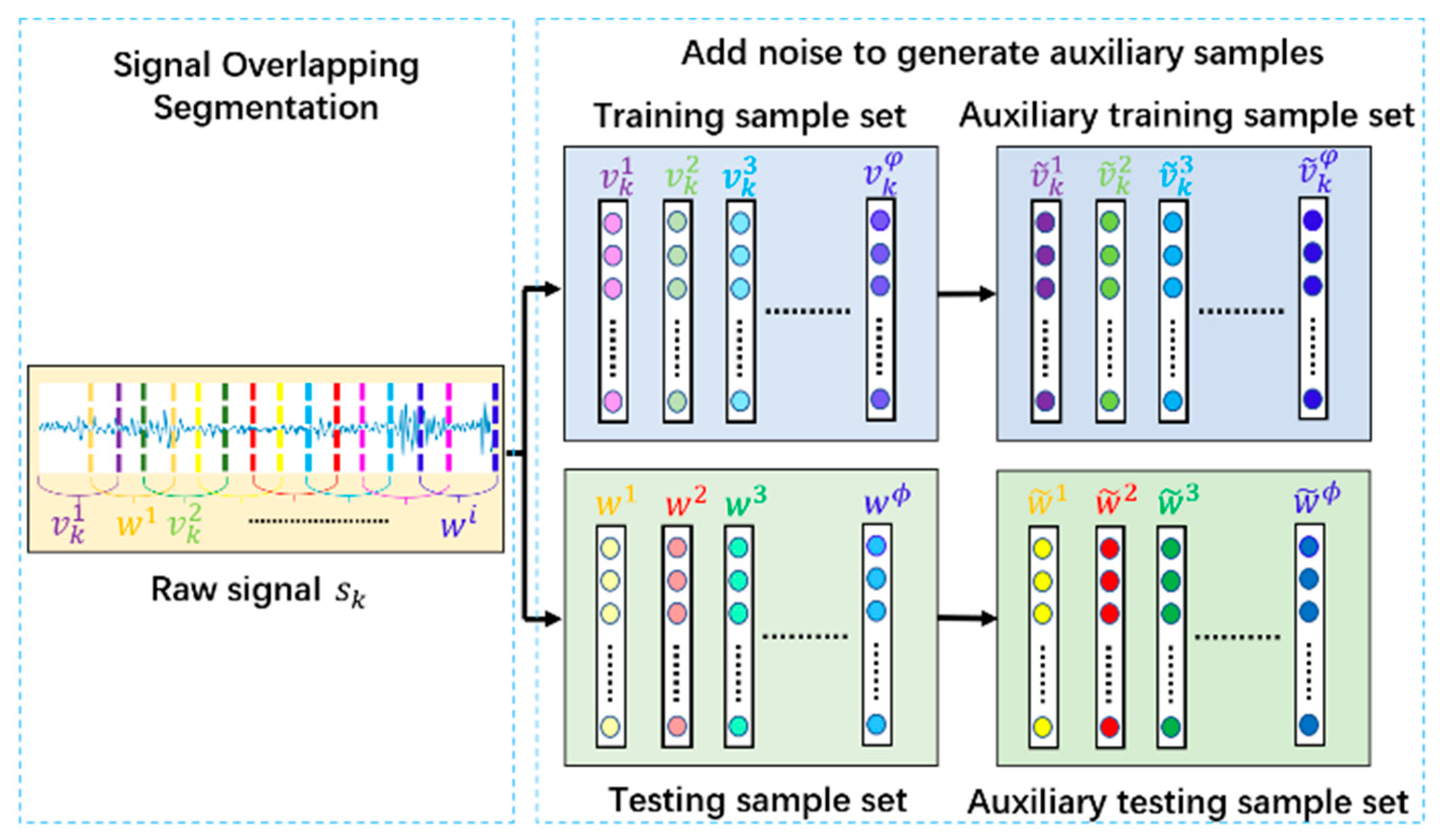
Data preprocessing plays a vital role in training the regularization parameter regression network model; the data preprocessing procedure is shown in Figure 1.
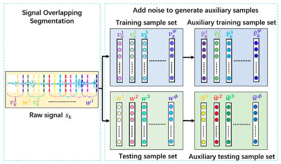
Figure 1.
Data preprocessing procedure.
As illustrated in Figure 1, there are different running states of rotating machines, and one running state stands for one type in the fault diagnosis task, and denotes the -th type of raw vibration signal (). Firstly, the overlapping segmentation sampling is executed on each type of raw vibration signal. Specifically, the overlapping sampling of is carried out with a sampling interval of . Then, the one-dimensional samples, and , represent the training samples and testing samples, respectively.
In order to accomplish the training of the regularization parameter regression network model, white Gaussian noise with the distribution is added to the samples to generate the corresponding auxiliary samples, and .
3.2. Training Regularization Parameter Regression Network Model
Multilayer perceptron (MLP) is one popular deep learning network [28], which is a fully connected network with multiple hidden layers. An MLP network can be applied in a regression problem, which focuses on the relationship between an output parameter and input parameters. When the depth of the MLP model is , the training process of the MLP network model aims to learn the bias term and the parametric matrix through minimizing the following optimization problem:
where is the -th input training sample, is the number of training samples, is the target regression value of the input sample , is a predefined loss function, and is formulated as a nonlinear activation function.
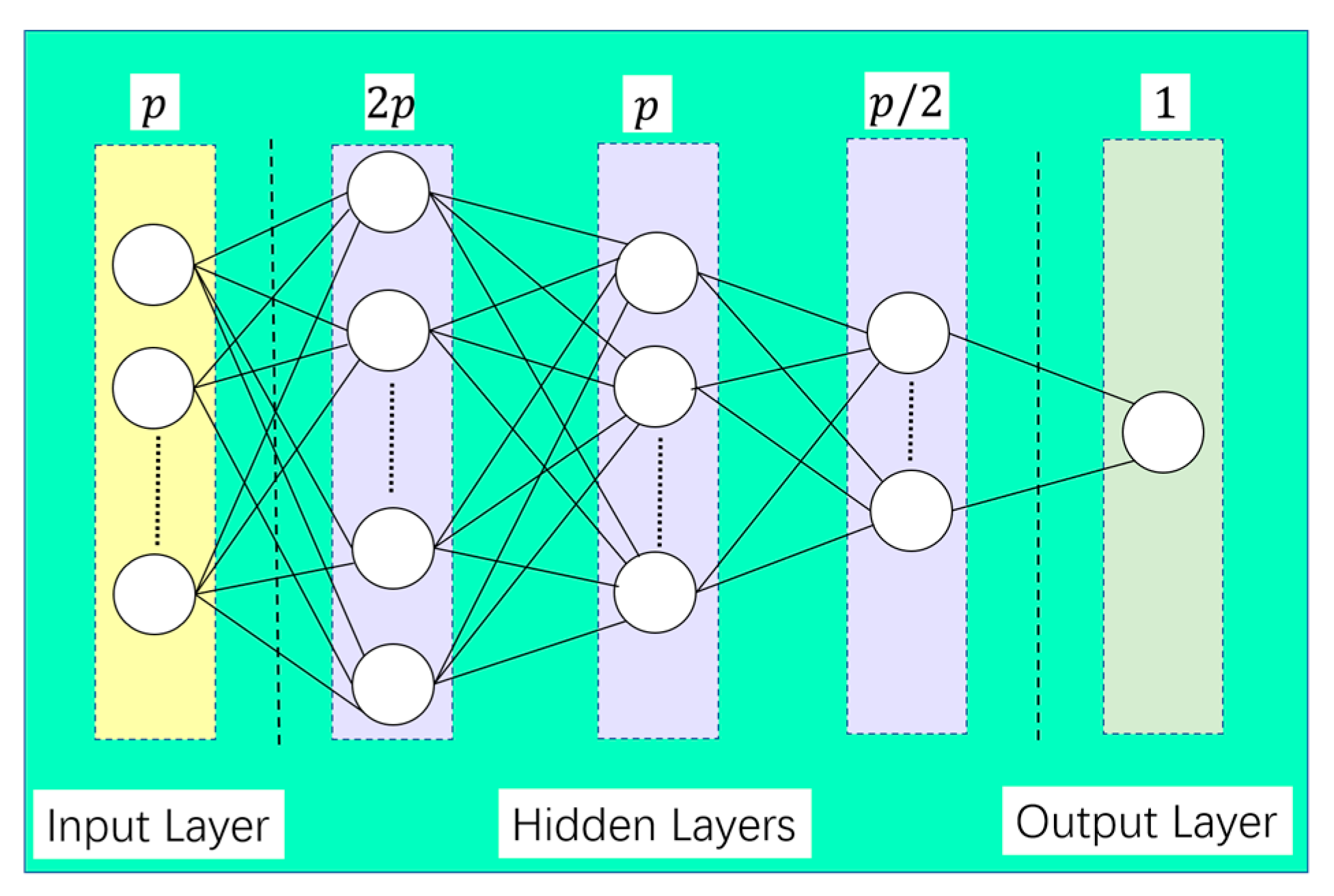
The SR-DEEP method constructs an MLP regression network for regressing regularization parameters. The specific network architecture of the MLP network is shown in Figure 2.

Figure 2.
Specific MLP network architecture.
It can be seen from Figure 2 that the input layer is composed of nodes, there are three hidden layers, and the numbers of nodes are , , and , respectively. The output layer is composed of a single node, which is the regularization parameter. The parameters of this network are randomly initialized using the Kaiming Uniform method. Based on the above constructed regularization parameter regression network, the specific training process is described in Figure 3.
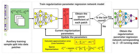
Figure 3.
Training regularization parameter regression network model.
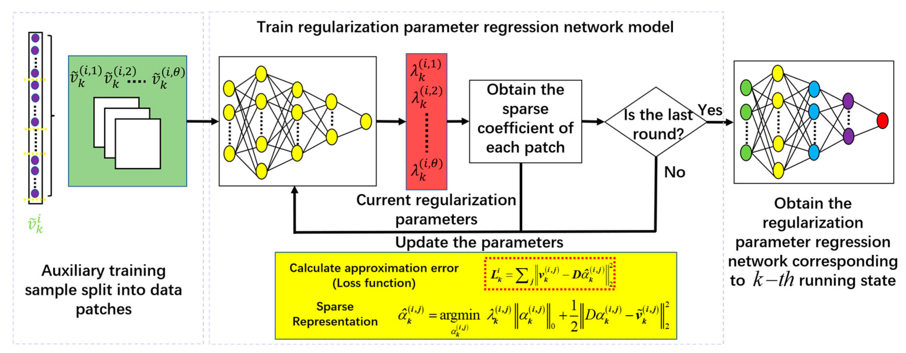
As depicted in Figure 3, the one-dimensional auxiliary training sample is converted into a two-dimensional vector, and then it is unfolded into data patches (, , ) to reduce the computational burden. These patches are fed into this MLP network to regress the corresponding regression parameter . Moreover, it is worth noting that the whole training process of the regularization parameter regression network is carried out by the sparse fault model. According to the sparse representation model, the approximate solution of the sparse coefficient vector is produced by denoising the auxiliary sample patch . The is defined as
where represents the current regularization parameter. comes from the trained regularization parameter regression network model, is constructed by the inverse discrete cosine transform, and ISTA is adopted to resolve the optimization problem of Equation (6). According to , the denoised data patch of is acquired. And the sparse reconstruction error function is between the original training samples and the sparse reconstruction denoised samples, which is simultaneously regarded as the mean squared error (MSE) loss function of the regularization parameter regression network. Then, the regularization parameter regression network is trained by updating the parameters of each layer using the back-propagation algorithm. Depending on the powerful mining ability of deep learning, the acquired regularization parameters contain the potential fault running state information.
In this paper, all training samples of the specific rolling bearing running state complete forward and backward propagations of training, that is, a complete model updating procession, which is called a training round.
3.3. Fault Classification
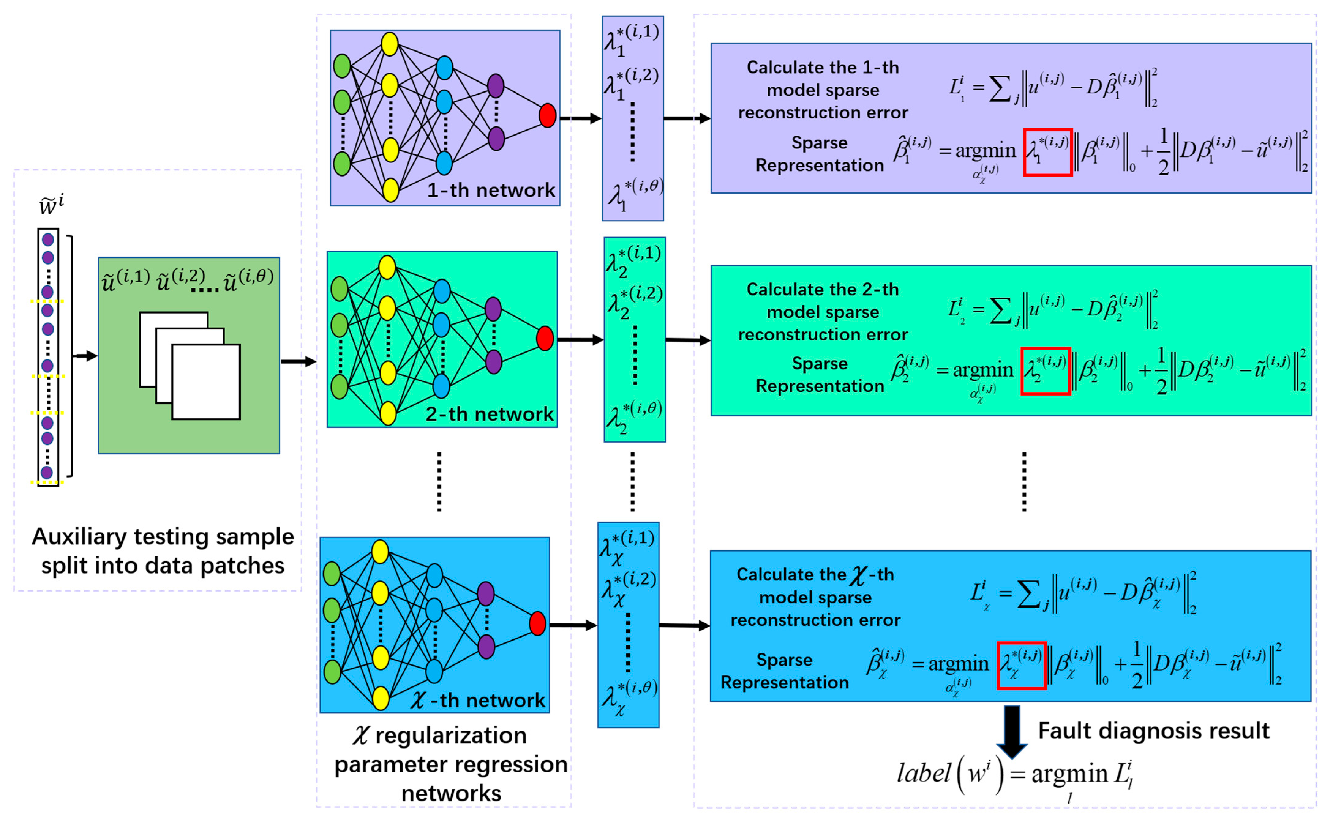
The central principle for the discrimination criterion of the sparse representation classification (SRC) method depends on the fact that signals of the same running state own similar sparse structures. According to this principle, the trained network models carry the specific knowledge of signal. Hence, the trained regularization parameter regression network models are introduced to the SRC method, which can better improve the performance of fault classification. Specifically, Figure 4 displays the proposed fault classification method.

Figure 4.
Illustration of fault classification.
Figure 4 illustrates the fault classification process for the testing sample . Firstly, regularization parameter regression network models are gained according to the training method in Section 3.2. The corresponding patches of the auxiliary testing sample are input into the regularization parameter regression network models, respectively. Then, the different types of regularization parameters are acquired for the current testing sample .
Secondly, the sparse coefficient vector for the testing sample patches is solved using the sparse representation fault model,
where represents the approximate solution of the -th classification sparse coefficient corresponding to the -th patch of the training sample. Based on , the sparse coefficient vector groups, , are obtained using Equation (7). The sparse reconstruction error is calculated between the original testing samples and the sparse reconstruction denoised testing samples .
Finally, the sparse reconstruction errors, , are obtained for the testing sample , respectively. On the principle of minimum approximation error, the running state of the testing sample is assigned with the minimum sparse reconstruction error, .
The above steps are repeated to classify all the testing samples.
4. The Proposed SR-DEEP Method for Fault Diagnosis
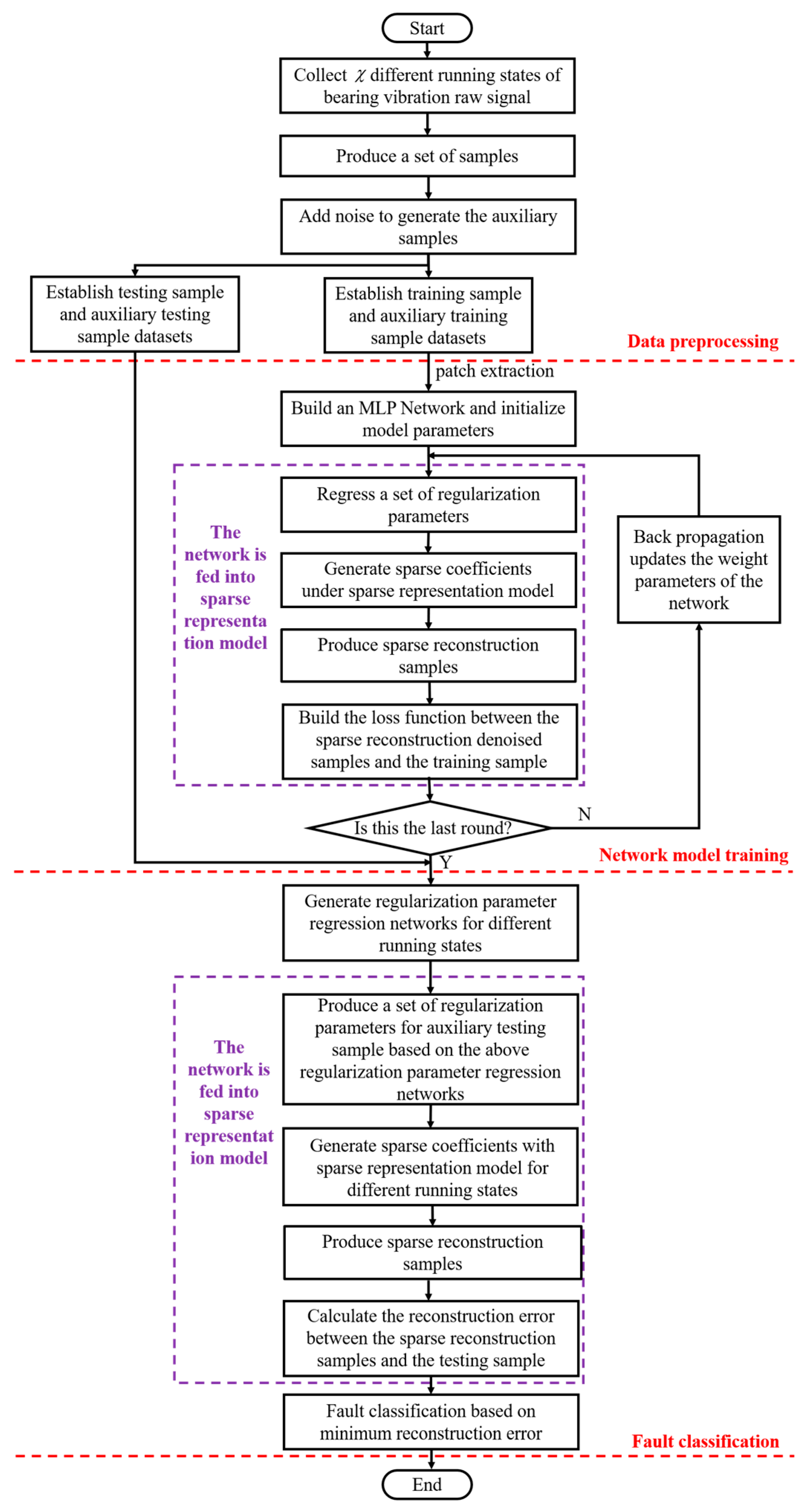
To sum up, Figure 5 shows the complete flow chart of the proposed SR-DEEP intelligent fault diagnosis method, which is mainly divided into three basic modules, which are data preprocessing, training regularization parameter regression network model, and fault classification. The overall steps of the SR-DEEP method are summarized below.
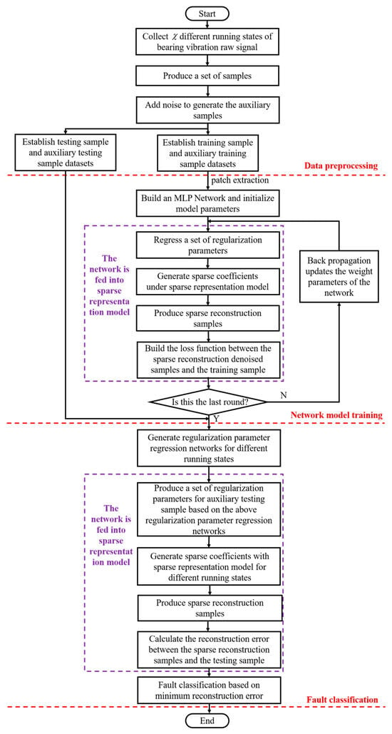
Figure 5.
The proposed SR-DEEP method flow chart.
Step 1: Collect different running states of bearing vibration raw signals. In this paper, two datasets from different experimental platforms are used to verify the effectiveness of the proposed SR-DEEP method, respectively.
Step 2: A set of samples is produced by overlapping the segmentation sampling.
Step 3: In order to train a regularization parameter regression network model, the corresponding auxiliary samples are generated by adding noise to these segmented samples.
Step 4: The samples are randomly divided into testing samples and training samples , respectively. Meanwhile, the corresponding auxiliary testing samples are , and the auxiliary training samples are .
Step 5: Based on the MLP network, the regularization parameter regression network is built and the model parameters are initialized. It is worth noting that the the regularization parameter regression network is trained via the sparse fault model.
Step 6: The auxiliary training samples are input into the regularization parameter regression network model to regress the corresponding regularization parameters.
Step 7: Sparse coefficients are generated based on the sparse fault model and used to produce sparse reconstructed denoised samples.
Step 8: The loss function is built between the sparse reconstruction denoised samples and training samples, .
Step 9: The back propagation updates the weight parameters of the network by minimizing the loss function.
Step 10: Steps 6–9 are repeated until the round times are reached, and the regularization parameter regression network model is generated for the -th running state.
Step 11: regularization parameter regression network models are generated for different fault running states, which are used for the final fault classification module.
Step 12: For each auxiliary testing sample, the set of regularization parameters is produced based on the trained regularization parameter regression network models, separately.
Step 13: The reconstruction errors between sparse reconstruction samples and the testing samples are calculated according to the above produced regularization parameters.
Step 14: On the principle of the minimum approximation error, the fault classification result is obtained.
5. Experiment and Analysis
In this section, the performance of the proposed SR-DEEP method was verified on two bearing datasets. The regularization parameter regression networks were implemented in the PyTorch environment. The experiment execution environment was described as Intel Core i5 7200U CPU@2.5GHz with 8 GB of memory.
5.1. Descriptions of Datasets
Two adopted bearing datasets were collected from two experimental platforms, respectively, which are shown in Figure 6. The detailed descriptions of the two experimental platforms are described as follows:

Figure 6.
The experimental platforms: (a) CWRU experimental platform; (b) QPZZ-II experimental platform.
- (1)
- CWRU platform: As shown in Figure 6a, the Case Western Reserve University (CWRU) [29] experimental platform is mainly composed of a driver, a load system, and a signal acquisition system. The selected bearing vibration signals were measured under the condition of an acceleration sensor sampling frequency of 12 kHz and a fault diameter of 0.007 inches. Additionally, the detailed parameters of this bearing dataset are presented in Table 1.
 Table 1. Details about the CWRU dataset.
 - (2)
- QPZZ-II platform: Figure 6b shows the QPZZ-II rotating machinery failure test platform. The rolling bearing of the N205 type in the rotating shafting was taken as a test object, and the faults of its components were machined via EDM. Additionally, the vibration signals of the different running states were collected using the USB-4431 data acquisition card, a vibration acceleration sensor, and the LabVIEW2018 software. The vibration signals were sampled at a sampling frequency of 12 kHz, and they are described in Table 2.
 Table 2. Details about the QPZZ-II dataset.
5.2. Parameter Setting
The experimental samples are obtained via overlapping segmentation sampling, which is performed on each vibration signal. The overlapping length of the adjacent samples is 80. Furthermore, to comprehensively verify the performance of the proposed SR-DEEP method, two data preprocessing methods are used for the segmented samples, which are described in detail as follows:
(1) Method 1: Each segmented sample is reshaped into a 128 × 128 two-dimensional sample. In this way, each running state of the rolling bearing signal is divided into 500 samples. Then, 432 samples are randomly selected to form a training sample set, and the resting 68 samples are used to construct a testing sample set.
(2) Method 2: Each segmented sample is reshaped into a 32 × 32 two-dimensional sample. In this way, each running state of the rolling bearing signal is divided into 2000 samples. Then, 1600 samples are randomly selected to form a training sample set, and the resting 400 samples are used to construct a testing sample set.
In Section 5.2 and Section 5.3, the experiments adopt method 1 of data preprocessing. Moreover, for a comparison with more methods, the experiments use method 2 of data preprocessing in Section 5.4. In this paper, fault diagnosis is solved using the trained regularization parameter regression network models, which are built on the MLP network, and its model parameters are listed in Table 3.

Table 3.
Definition of network parameters.
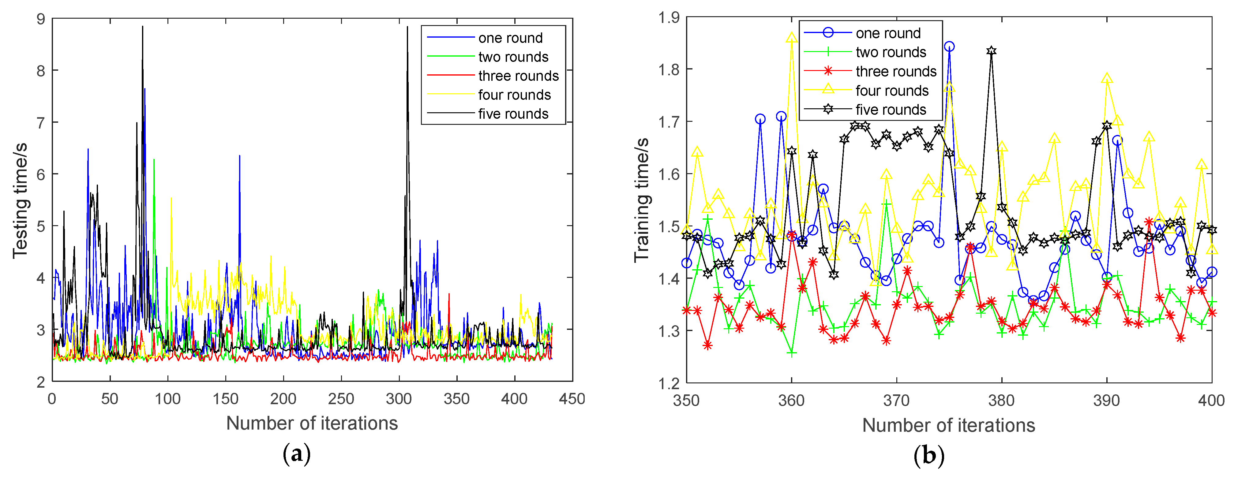
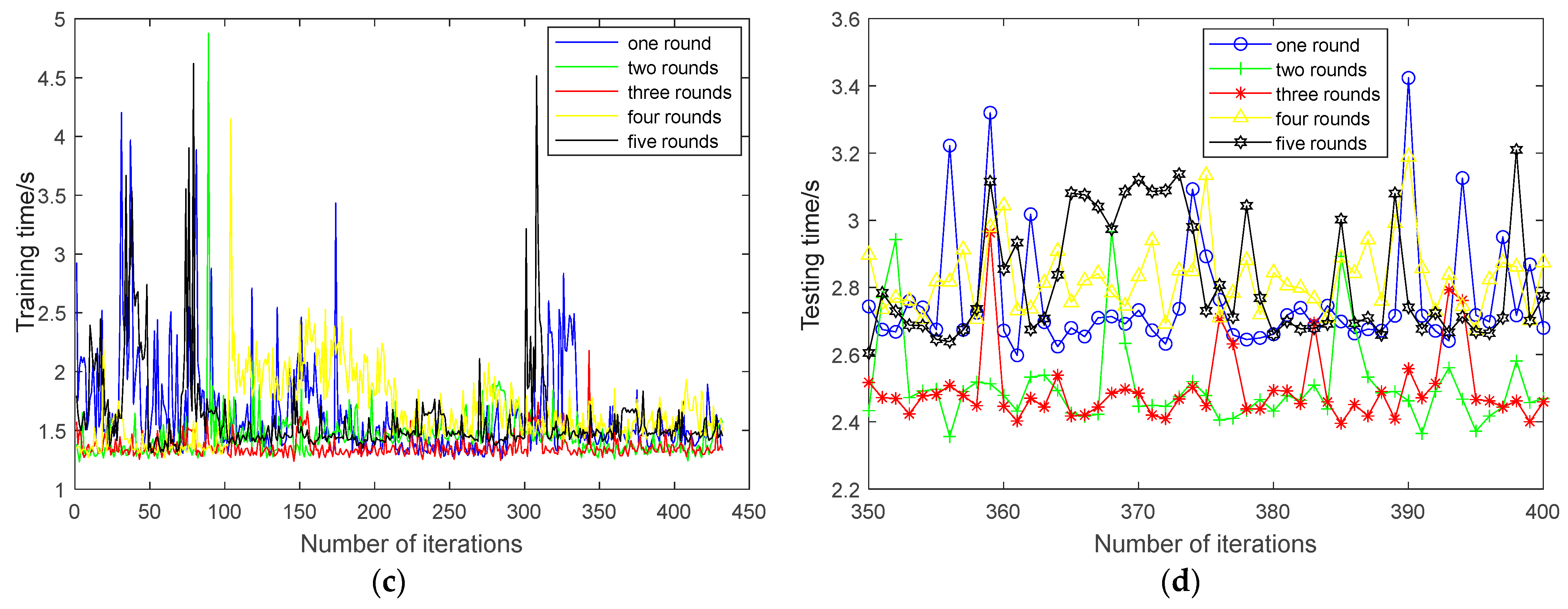
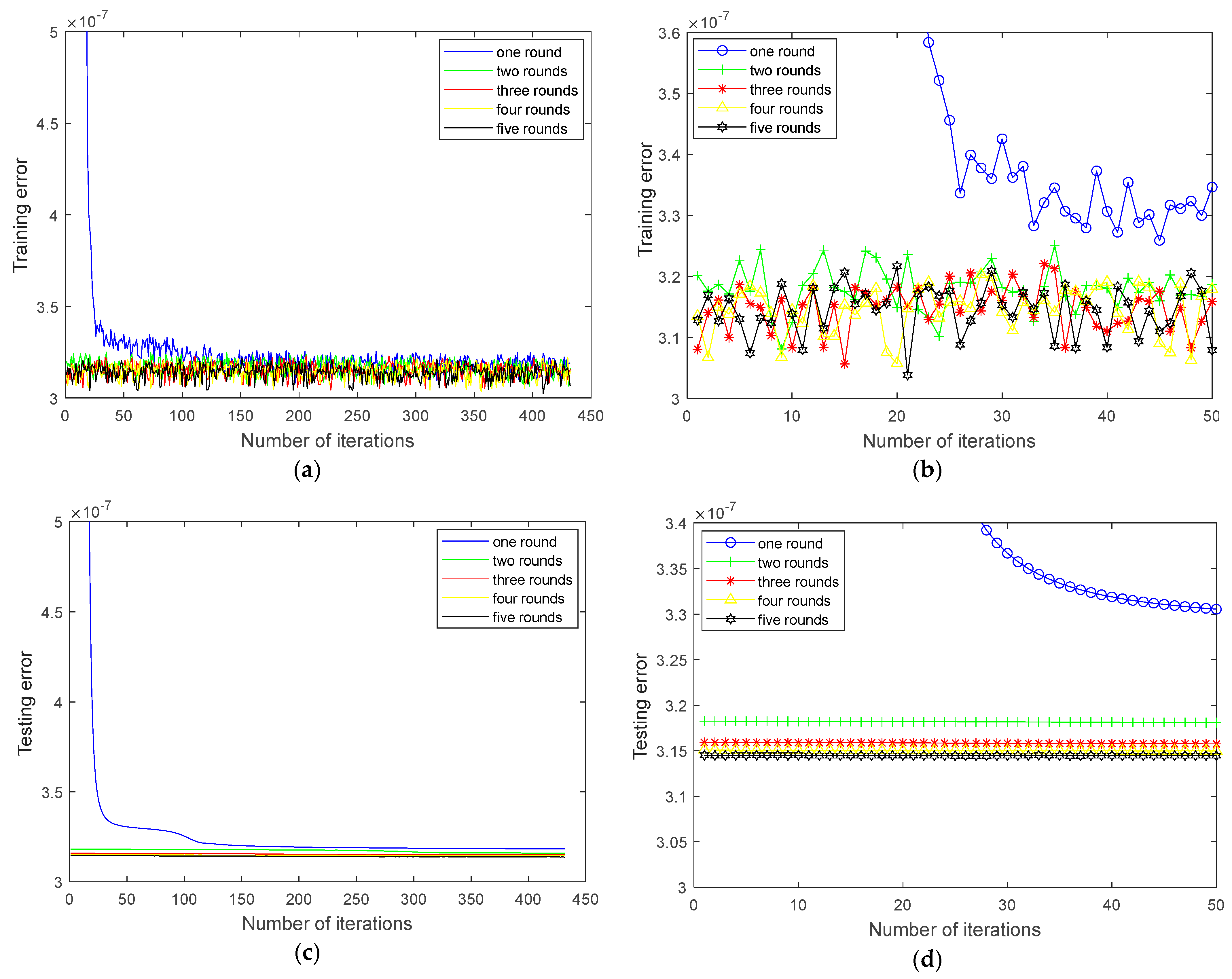
In order to train these network models, Gaussian noise with a mean of 0 and a variance of 0.5 is added to each sample. After that, the corresponding auxiliary sample is generated. In the process of training the network models, each two-dimensional sample is folded into a group of patches with the size of (). Also, the MSE loss function is minimized by the Adam optimizer [19] to gradually update the network parameter values. Furthermore, the number of training rounds has a significant effect on the fault diagnosis performance of SR-DEEP. In this section, five values of rounds (i.e., 1, 2, 3, 4, and 5) are chosen to demonstrate their impacts on the training model when the learning rate is set as 0.0001 and the batch size is set as 1. The four indicator values with respect to the five rounds are summarized in Figure 7 and Figure 8.
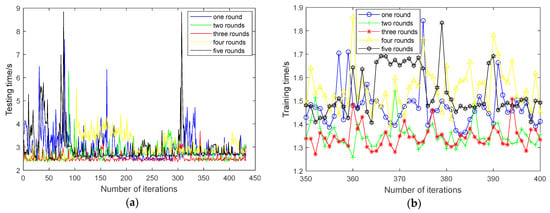
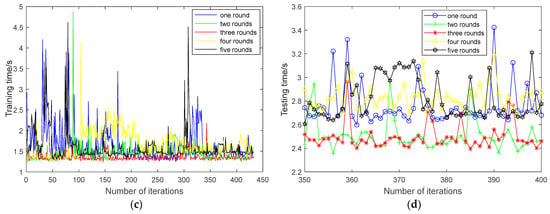
Figure 7.
Time variation trend of inner ring fault regularization parameter regression network. (a) Training time trend; (b) zoomed-in view of (a); (c) testing time trend; (d) zoomed-in view of (c).
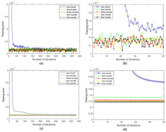
Figure 8.
Loss variation trend of inner ring fault regularization parameter regression network. (a) Training error trend; (b) zoomed-in view of (a); (c) testing error trend; (d) zoomed-in view of (b).
In the process of training the regularization parameter regression network, 432 training samples are all iterated once in each round. After a sample is sent to the memory to complete an iteration, 5 samples are randomly selected from 68 testing samples (only for testing, and not participating in model training). Then, the training and testing errors are used to confirm the current training situation of this iteration. As shown in Figure 7 and Figure 8, when the number of rounds increases, the overall trends of time and error of the inner ring fault decrease. To illustrate the linear trend more clearly, these plots in the right panel are zoomed-in views of the plots in the left panel. It can be seen from Figure 7a,c that when the training process reaches the third round, compared with the first round, the training and testing times are significantly reduced. And they are slightly better than the second round. In addition, as shown in Figure 8, when the training process reaches the third round, the errors of the training and testing samples are significantly lower than those of the first round and the second round, and have little change compared with those of the fourth round and the fifth round. The above results preliminarily show that when the network training reaches the third round, the network model has been trained effectively. Therefore, the number of network training rounds is set as three rounds for the other experiments in this paper.
5.3. Fault Classification Results of SR-DEEP
5.3.1. CWRU Dataset
The classification results of SR-DEEP have all reached 100.00% for the four running states of CWRU dataset based on method 1 of data preprocessing. It is clear that SR-DEEP exhibits an outstanding performance, which indicates the effectiveness of combining sparse representation and deep learning. The training times of the regression network model after three rounds of training are listed in Table 4.

Table 4.
Regularization parameter regression network training time for CWRU Dataset/s.
Table 4 shows that it is very time-consuming to train a regularization parameter regression network, which is due to the lack of more powerful computing power in this paper. These running times can be further improved by GPU.
5.3.2. QPZZ-II Dataset
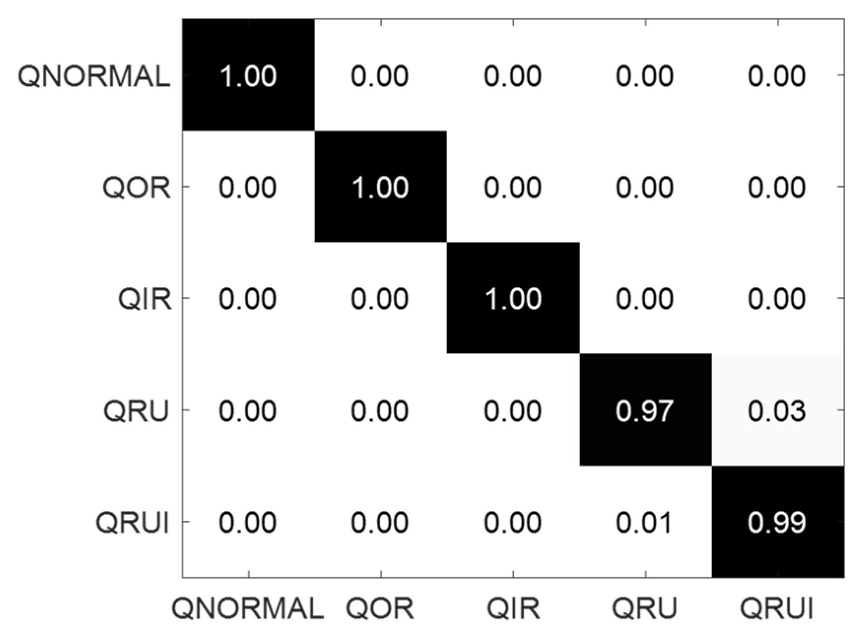
In this section, the experiments are conducted on the QPZZ-II dataset based on method 1 of data preprocessing. The final testing results of SR-DEEP are shown in Figure 9.

Figure 9.
Classification confusion matrix of QPZZ-II experimental dataset.
The training times of five running state regularized parameter regression networks are shown in Table 5.

Table 5.
Regularization parameter regression network training time for QPZZ-II Dataset/s.
The confusion matrix of the SR-DEEP fault classification results is shown in Figure 9, and the overall fault classification accuracy is up to 99.20%. The results show that the network fault prediction accuracy could reach 100% in the running states of QNORMAL, QOR, and QIR. In the running states of QRU and QRUI, the fault classification accuracy reached 97.00% and 99.00%, respectively.
Compared to the CWRU dataset, the QPZZ-II dataset is affected by more interference. Hence, the fault classification accuracy decreases, but it is still very high, indicating that the algorithm has a good generalization ability. Similar to Table 4, Table 5 demonstrates that the proposed method is time-consuming under the current running environment. In addition, the two datasets come from different rotating speeds, and the two experimental results verify the applicability of the method under varying speed conditions.
5.4. Comparative Experiment Analysis
5.4.1. Comparison with the SRC Method
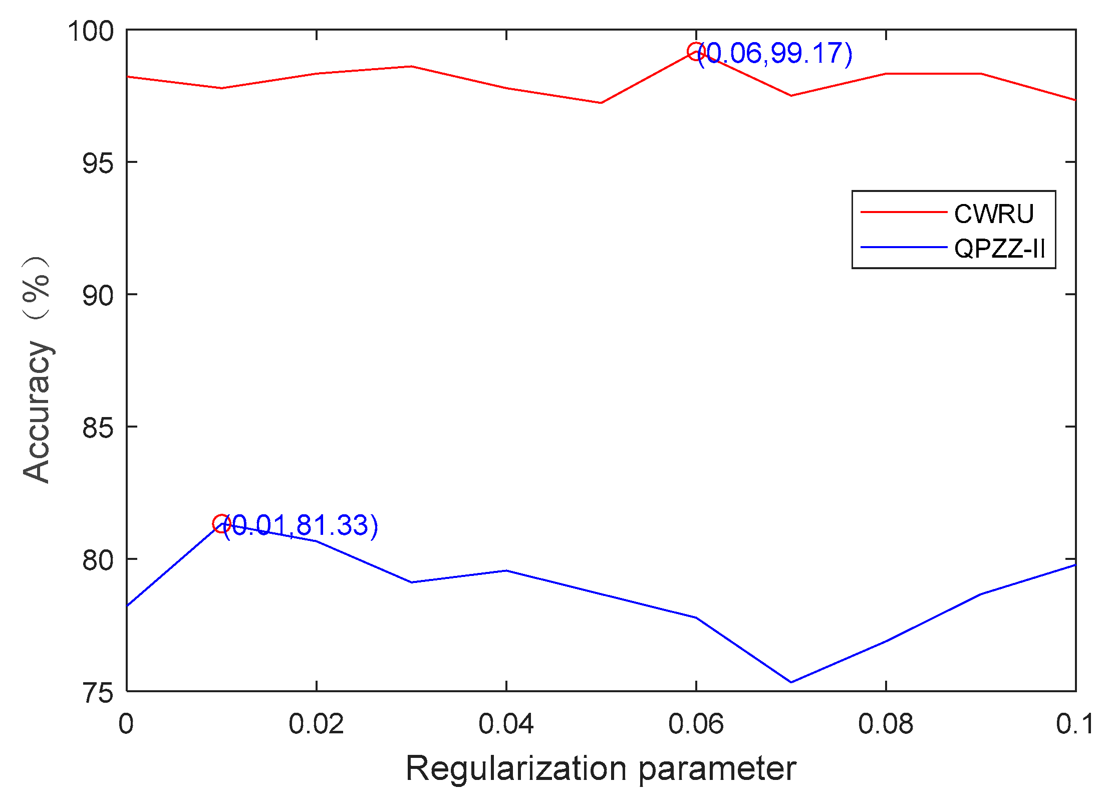
(1) To illustrate the effect of the regularization parameter on the fault classification accuracy, these experiments were performed based on the SRC method and the Fast Iterative Shrinkage Thresholding Algorithm (FISTA) [26]. These experiments directly adopt the original CWRU dataset without fault feature extraction and are implemented on the number of regularization parameters from 0 to 0.1 with the interval of 0.01. The final classification accuracies for different regularization parameter values are shown in Figure 10.

Figure 10.
Fault classification accuracies based on SRC-FISTA/%.
It can be seen from Figure 10 that the accuracies of fault classification fluctuate with the increase in the regularization parameter. Hence, it is very important for fault diagnosis to set the suitable regularization parameter value, which also shows the necessity of the research on the regularization parameter in this paper.
(2) In this subsection, four comparative methods are compared to demonstrate the superiority of the proposed SR-DEEP method for fault classification. Among them are Orthogonal Matching Pursuit (OMP) [23], Original Augmented Lagrange (OAL) [30], Homotopy [31], and Two-Phase Test Sample Sparse Representation (TPTSR) [32]. Significantly, these comparative methods adopt the SRC method with different optimization algorithms. The experiment results are acquired and listed in Table 6.

Table 6.
Comparison results of SRC methods/%.
It can be seen from Table 6 that the average classification accuracies of the four methods do not reach 99.20% in two datasets. Nevertheless, the classification accuracies of SR-DEEP reached 100.00% and 99.20%, respectively. These results indicate that the SR-DEEP method possesses a better classification ability compared to the four comparative methods.
Notably, as shown in Figure 10 and Table 6, the fault diagnosis results of the SR-DEEP method are improved by 0.83% and 17.87%, respectively, compared with the SRC-FISTA method based on the optimal regularization parameters, which indicates the effectiveness of the regularization parameter self-adaptation strategy.
To sum up, the main reason for the lower recognition performances of the sparsity-based methods is that they identify the rolling bearing running states by finding the minimum sparse reconstruction error. But the fixed values of the regularization parameter limit the differences in the sparse reconstruction errors of the different running states. Furthermore, it should be noted that the computational cost of the sparsity-based method is commonly lower than that of the SR-DEEP method due to the calculation of the regularization parameters using the regularization parameter network models.
5.4.2. Comparison with DEEP Learning Methods
To prove the effectiveness of SR-DEEP, SR-DEEP was compared with seven intelligent diagnosis methods based on deep learning models, including AE, SAE, CNN, LeNet, ResNet18, LSTM, and MLP in ref. [10]. To avoid the influence of super-parameters, two sets of experiments were conducted on two datasets by shaping time domain samples into 2D samples. The specific information for these experiments includes the first group of experiments: epoch = 3 and learning rate = 0.0001. In addition, it is worth noting that the batch size of the MLP algorithm is set to 2, but the batch size of the other algorithms is set to 1; in the second group of experiments, the batch size = 64, epoch = 5, and the learning rate = 0.001. Finally, the averages of the accuracies obtained using the last epoch are presented in Table 7 and Table 8.

Table 7.
Comparison results of deep learning classification methods on CWRU/%.

Table 8.
Comparison results of deep learning classification methods on QPZZ-II/%.
As shown in Table 7, the average diagnostic accuracy of SR-DEEP is 99.38%, which outperforms AE, SAE, CNN, LeNet, ResNet18, LSTM, and MLP by 3.72%, 10.85%, 15.85%, 0.19%, 11.72%, 57.00%, and 31.44%, respectively. In addition, it can be seen from Table 8 that the average diagnostic accuracy of SR-DEEP is 89.53%, which outperforms AE, SAE, CNN, LeNet, ResNet18, LSTM, and MLP by 2.50%, 3.80%, 29.23%, 11.75%, 3.25%, 50.485, and 23.10%, respectively. These comparison results demonstrate that the proposed SR-DEEP method achieves better accuracy than the compared networks and is also more robust than deep learning fault diagnosis methods. More importantly, through embedding the MLP network into sparse representation, the SR-DEEP method has improved the fault diagnosis results by 31.44% and 23.10% compared to the intelligent diagnosis methods based on the MLP network, indicating the feasibility of embedding a deep learning network into a sparse representation model.
To sum up, the common deep learning diagnosis methods both achieve fault diagnosis by mining data, but they ignore the structured prior knowledge of the rolling bearing vibration signal, thus restricting their representations and discrimination abilities for rolling bearing fault diagnosis. Furthermore, it should be noted that the above experiments were conducted on fixed parameters. Hence, if the parameters change, especially when the number of network layers increases, the superiority of the SR-DEEP method may be affected.
6. Conclusions
This paper introduces a novel intelligent fault diagnosis method called SR-DEEP, which embeds the MLP network into a sparse representation model. Firstly, based on the MLP network, the regularization parameter regression network models used for specific fault running states are trained separately based on a sparse representation model, which carries the discriminative information for the fault running state. Secondly, for the testing samples, the regularization parameters for different fault running states can be generated using different network models. Thirdly, depending on the obtained regularization parameters, the testing samples are classified by means of the SRC method. The SR-DEEP method is a new endeavor for combining the model-driven sparse representation method with the data-driven deep learning method. Through mining the potential relationship between the regularization parameters and running states, SR-DEEP not only improves the adaptability of sparse regularization parameters but also enhances the accuracy of rolling bearing fault diagnosis.
Finally, fault diagnosis experiments are conducted on two bearing fault datasets; the overall average classification accuracies of SR-DEEP method reach 100.00% and 99.2% individually. Compared with the traditional SRC methods on the CWRU dataset, the average classification accuracies of SR-DEEP are increased by 2.57%, 2.17%, 3.46%, and 0.83%, respectively. Meanwhile, the classification accuracies of SR-DEEP are increased by 2.50%, 3.80%, 29.23%, 11.75%, 3.25%, 50.485, and 23.10%, respectively, compared with the classical deep learning classification methods on the QPZZ-II dataset. These results verify the performance of the proposed SR-DEEP method for fault diagnosis.
Future works will focus on improving the performance of the regularization parameter regression network model to further improve fault classification accuracy and reduce the computational cost. Furthermore, the effectiveness of the SR-DEEP method needs to be further validated on more types of experiments, such as different loads, different fault severity levels and sensitivity analyses, and so on.
Author Contributions
Conceptualization, Y.N. and Y.W. (Yuchun Wang); methodology, Y.N. and P.Z.; software, Y.N., G.W. and W.D.; validation, Y.N., X.Z. and W.D.; formal analysis, W.D.; resources, Y.N. and Y.W. (Yuchun Wang); data curation, W.D.; writing—original draft preparation, Y.W. (Yanjuan Wang); writing—review and editing, P.Z. and Y.W. (Yuchun Wang); visualization, G.W. and X.Z.; funding acquisition, Y.N. All authors have read and agreed to the published version of the manuscript.
Funding
This work was supported by the National Natural Science Foundation of China under Grant 62276042, the National Natural Science Foundation of China under Grant 52372436, the Liaoning Provincial Department of Education Scientific Research Funding Project under Grant LJKZ0481, the Natural Science Foundation of Sichuan Province 2022NSFSC1941, the Special Program of Huzhou 2023GZ05, and the Foundation of Yunnan Key Laboratory of Service Computing No. YNSC23118.
Data Availability Statement
Not applicable.
Conflicts of Interest
The authors declare no conflict of interest.
References
- Zhao, Z.B.; Wu, J.Y.; Li, T.F.; Sun, C.; Chen, X.F. Challenges and opportunities of AI-enabled monitoring, diagnosis & prognosis: A review. Chin. J. Mech. 2021, 34, 56. [Google Scholar]
- Feng, Z.; Zhou, Y.; Zuo, M.J.; Chu, F.; Chen, X. Atomic decomposition and sparse representation for complex signal analysis in machinery fault diagnosis: A review with examples. Measurement 2017, 103, 106–132. [Google Scholar] [CrossRef]
- Zhang, Z.; Huang, W.; Liao, Y.; Song, Z.; Shi, J.; Jiang, X.; Shen, C.; Zhu, Z. Bearing fault diagnosis via generalized logarithm sparse regularization. Mech. Syst. Signal Process. 2022, 167, 108576. [Google Scholar] [CrossRef]
- Li, J.; Tao, J.; Ding, W.; Zhang, J.; Meng, Z. Period-assisted adaptive parameterized wavelet dictionary and its sparse representation for periodic transient features of rolling bearing faults. Mech. Syst. Signal Process. 2022, 169, 108796. [Google Scholar] [CrossRef]
- Zhao, Z.; Wu, S.; Qiao, B.; Wang, S.; Chen, X. Enhanced sparse period-group lasso for bearing fault diagnosis. IEEE Trans. Ind. Electron. 2019, 66, 2143–2153. [Google Scholar] [CrossRef]
- Zhao, Z.; Wang, S.; An, B.; Guo, Y.; Chen, X. Hierarchical hyper-Laplacian prior for weak fault feature enhancement. ISA Trans. 2020, 96, 429–443. [Google Scholar] [CrossRef]
- Qin, Y.; Zou, J.Q.; Tang, B.P.; Wang, Y.; Chen, H.Z. Transient feature extraction by the improved orthogonal matching pursuit and K-SVD algorithm with adaptive transient dictionary. IEEE Trans. Ind. Inform. 2019, 16, 215–227. [Google Scholar] [CrossRef]
- Zeng, M.; Chen, Z. SOSO Boosting of the K-SVD denoising algorithm for enhancing fault-induced impulse responses of rolling element bearings. IEEE Trans. Ind. Electron. 2020, 67, 1282–1292. [Google Scholar] [CrossRef]
- Niu, Y.J.; Li, H.; Deng, W.; Fei, J.Y.; Li, S.Y.; Bo, L.Z. Rolling bearing fault diagnosis method based on TQWT and sparse representation. J. Traffic Transp. 2021, 21, 237–246. [Google Scholar]
- Li, Q. A comprehensive survey of sparse regularization: Fundamental, state-of-the-art methodologies and applications on fault diagnosis. Expert Syst. Appl. 2023, 229, 120517. [Google Scholar] [CrossRef]
- You, X.L.; Li, J.C.; Deng, Z.W.; Zhang, K.; Yuan, H. Fault Diagnosis of Rotating Machinery Based on Two-Stage Compressed Sensing. Machines 2023, 11, 242. [Google Scholar] [CrossRef]
- Huang, X.; Zhang, X.D.; Xiong, Y.W.; Dai, F.; Zhang, Y.J. Intelligent fault diagnosis of turbine blade cracks via multiscale sparse filtering and multi-kernel support vector machine for information fusion. Adv. Eng. Inform. 2023, 56, 101979. [Google Scholar] [CrossRef]
- Zhao, Z.B.; Li, T.F.; An, B.T.; Wang, S.B.; Ding, B.Q.; Yan, R.Q.; Chen, X.F. Model-driven deep unrolling: Towards interpretable deep learning against noise attacks for intelligent fault diagnosis. ISA Trans. 2022, 129, 644–662. [Google Scholar] [CrossRef]
- Miao, M.; Sun, Y.; Yu, J. Deep sparse representation network for feature learning of vibration signals and its application in gearbox fault diagnosis. Knowl.-Based Syst. 2020, 240, 108116. [Google Scholar] [CrossRef]
- Ma, H.; Li, S.; Lu, J.; Zhang, Z.; Gong, S. Structured sparsity assisted online convolution sparse coding and its application on weak signature detection. Chin. J. Aeronaut. 2022, 35, 266–276. [Google Scholar] [CrossRef]
- Zhao, M.; Zhong, S.; Fu, X.; Tang, B.; Pecht, M. Deep residual shrinkage networks for fault diagnosis. IEEE Trans. Ind. Inf. 2019, 16, 4681–4690. [Google Scholar] [CrossRef]
- Zhou, X.; Zhou, H.; Wen, G.; Huang, X.; Lei, Z.; Zhang, Z.; Chen, X. A hybrid denoising model using deep learning and sparse representation with application in bearing weak fault diagnosis. Measurement 2021, 189, 110633. [Google Scholar] [CrossRef]
- Gregor, K.; Lecun, Y. Learning fast approximations of sparse coding. In Proceedings of the 27th International Conference on International Conference on Machine Learning, Boston, MA, USA, 21 June 2010; pp. 399–406. [Google Scholar]
- Monga, V.; Li, Y.; Eldar, Y.C. Algorithm unrolling: Interpretable, efficient deep learning for signal and image processing. IEEE Signal. Proc. Mag. 2021, 38, 18–44. [Google Scholar] [CrossRef]
- Selesnick, I. Sparse Regularization via Convex Analysis. IEEE Trans. Signal Process. 2017, 65, 4481–4494. [Google Scholar] [CrossRef]
- Ma, S.; Han, Q.K.; Chu, F.L. Sparse representation learning for fault feature extraction and diagnosis of rotating machinery. Expert Syst. Appl. 2023, 232, 120858. [Google Scholar] [CrossRef]
- Wen, H.R.; Guo, W.; Li, X. A novel deep clustering network using multi-representation autoencoder and adversarial learning for large cross-domain fault diagnosis of rolling bearings. Expert Syst. Appl. 2023, 225, 120066. [Google Scholar] [CrossRef]
- Tropp, J.A.; Gilbert, A.C. Signal Recovery from Random Measurements via Orthogonal Matching Pursuit. IEEE Trans. Inform. Theory 2007, 53, 4655–4666. [Google Scholar] [CrossRef]
- Daubechies, I.; Defrise, M.; Mol, C.D. An iterative thresholding algorithm for linear inverse problems with a sparsity constraint. Commun. Pur. Appl. 2004, 57, 1413–1457. [Google Scholar] [CrossRef]
- Rakotomamonjy, A. Surveying and comparing simultaneous sparse approximation (or group-lasso) algorithms. Signal Process. 2011, 91, 1505–1526. [Google Scholar] [CrossRef]
- Beck, A.; Teboulle, M. A fast iterative shrinkage-thresholding algorithm for linear inverse problems. SIAM J. Imaging Sci. 2009, 2, 183–202. [Google Scholar] [CrossRef]
- Afonso, M.V.; Bioucas-Dias, J.M.; Figueiredo, M.A.T. Fast image recovery using variable splitting and constrained optimization. IEEE Trans. Image Process. 2010, 19, 2345–2356. [Google Scholar] [CrossRef]
- Rumelhart, D.E.; Hinton, G.E.; Williams, R.J. Learning internal representations by error propagation. In Readings in Cognitive Science; Morgan Kaufmann: San Francisco, CA, USA, 1998; pp. 399–421. [Google Scholar]
- Smith, W.A.; Randall, R.B. Rolling element bearing diagnostics using the Case Western Reserve University data: A benchmark study. Mech. Syst. Signal Process. 2015, 64–65, 100–131. [Google Scholar] [CrossRef]
- Yang, A.Y.; Zhou, Z.; Ganesh, A.; Sastry, S.S.; Ma, Y. Fast l1-minimization algorithms for robust face recognition. IEEE Trans. Image Process. 2013, 22, 3234–3246. [Google Scholar] [CrossRef]
- Asif, M.S. Primal Dual Pursuit: A Homotopy Based Algorithm for the Dantzig Selector; Georgia Institute of Technology: Atlanta, GA, USA, 2008; pp. 19–29. [Google Scholar]
- Xu, Y.; Zhang, D.; Yang, J.; Yang, J.Y. A two-phase test sample sparse representation method for use with face recognition. IEEE Trans. Circ. Syst. Vid. 2011, 21, 1255–1262. [Google Scholar]
Disclaimer/Publisher’s Note: The statements, opinions and data contained in all publications are solely those of the individual author(s) and contributor(s) and not of MDPI and/or the editor(s). MDPI and/or the editor(s) disclaim responsibility for any injury to people or property resulting from any ideas, methods, instructions or products referred to in the content. |
© 2023 by the authors. Licensee MDPI, Basel, Switzerland. This article is an open access article distributed under the terms and conditions of the Creative Commons Attribution (CC BY) license (https://creativecommons.org/licenses/by/4.0/).

