Abstract
Potato malformation seriously affects commercial value, and its removal has become one of the core steps in the post-harvest and pre-sales process of potatoes. At present, this work mainly relies on manual visual inspection, which requires a lot of labor and incurs high investment costs. Therefore, precise and efficient automatic detection technology urgently needs to be developed. Due to the efficiency of deep learning based on image information in the field of complex object feature extraction and pattern recognition, this study proposes the use of the YOLOv3 algorithm to undertake potato malformation classification. However, the target box regression loss function MSE of this algorithm is prone to small errors being ignored, and the model code is relatively large, which limits its performance due to the high demand for computing hardware performance and storage space. Accordingly, in this study, CIOU loss is introduced to replace MSE, and thus the shortcoming of the inconsistent optimization direction of the original algorithm’s loss function is overcome, which also significantly reduces the storage space and computational complexity of the network model. Furthermore, deep separable convolution is used instead of traditional convolution. Deep separable convolution first convolves each channel, and then combines different channels point by point. With the introduction of an inverted residual structure and the use of the h-swish activation function, deep separable convolution based on the MobileNetv3 structure can learn more comprehensive feature representations, which can significantly reduce the computational load of the model while improving its accuracy. The test results showed that the model capacity was reduced by 66%, mAP was increased by 4.68%, and training time was shortened by 6.1 h. Specifically, the correctness rates of malformation recognition induced by local protrusion, local depression, proportional imbalance, and mechanical injury within the test set range were 94.13%, 91.00%, 95.52%, and 91.79%, respectively. Misjudgment mainly stemmed from the limitation of training samples and the original accuracy of the human judgment in type labeling. This study lays a solid foundation for the final establishment of an intelligent recognition and classification picking system for malformed potatoes in the next step.
1. Introduction
Potato is the staple food for most developing countries worldwide and thus has great significance for food security, poverty reduction, and wealth accumulation [1]. However, the market value of the malformed potato is nearly nonexistent, and mixed sales seriously affect overall income. Therefore, the removal of malformed potatoes has become one of the core processes of post-harvest and pre-sales treatment. At present, this work mainly relies on manual selection, which has the disadvantages of difficult unification of standards, high labor intensity, and high input costs. Therefore, an accurate, fast, efficient, and intelligent system for recognizing and screening malformed potatoes needs to be developed urgently.
In recent years, deep learning technology has developed rapidly. A target detection algorithm based on this technology does not need to require complex manual feature design. It can automatically extract various abstract features in an image and can be used for target classification according to the extracted results, which greatly improves the efficiency of target detection [2,3,4,5,6,7,8]. At present, deep learning has been widely applied in industry [9,10] and the military [11,12]. Now, its application in agriculture is urgently required and holds the potential to make a valuable contribution.
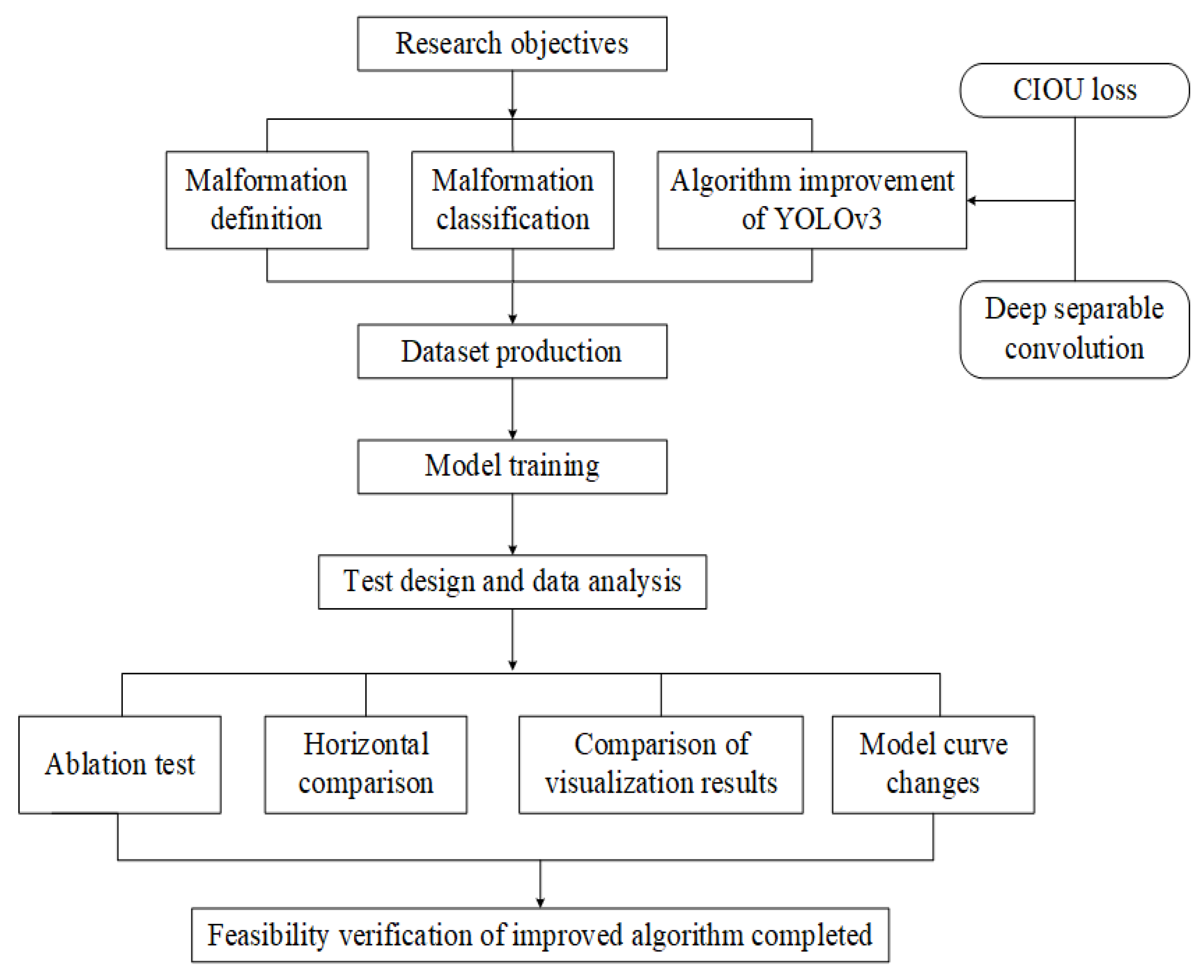
Deep learning originates from initial interpretations by humans, which are made based on human neural networks and neural models. It is a multi-layer neural network learning algorithm that completes the fitting of complex multidimensional spaces by learning nonlinear features of multi-layer network structures [13,14]. Typical specific applications, such as those outlined in Temniranrat et al. [15], involve the use of the YOLOv3 algorithm for rice disease detection and deploy it to a server. A kind of integrated multiple convolutional neural network for the disease and pest detection of coffee crops has been introduced in the literature [16]. This network is not only able to achieve good detection results but is also suitable for client deployment. As the third version of the YOLO series, the YOLOv3 algorithm is mainly used to detect the features of an acquired image, and its ability to detect large targets is significant [17]. Generally, detection speed and accuracy are able to meet requirements. However, the MSE loss function used in the target box regression is sensitive to the size of the identified object itself, which often leads to the neglect of small features. Therefore, the accuracy of the model still needs to be improved. In addition, the basic YOLOv3 algorithm model still has a large capacity, which increases the demand for computer storage space and, additionally, reduces the running speed of the model and the reliability of the results indirectly. Consequently, based on YOLOv3, this study improves the algorithm to enable more detailed and deeper malformation identification in order to achieve the accurate detection of different types of malformed potatoes. The technical process is shown in Figure 1.
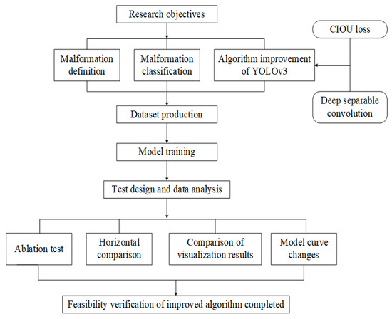
Figure 1.
Technical process.
First, the introduction of CIOU loss for regression loss optimization was proposed, and the dilemma of the inconsistent optimization direction of MSE loss was eliminated. CIOU loss not only made the target frame more stable but also had a faster convergence speed and higher accuracy. On this basis, deep separable convolution was used instead of traditional convolution, overcoming the problem of high computational intensity and model storage space in the YOLOv3 algorithm. Then, the test dataset was prepared and the test model was built. Going a step further, the model before and after the algorithm improvement was trained, and the loss function change curve of the model was compared. In the end, different test data analyses were conducted on the improved algorithm, including the following:
- (1)
- In order to obtain a higher-performance potato malformed object detection algorithm, the results of different modules before and after the improvement were compared.
- (2)
- To test the effectiveness of the improved algorithm, a horizontal comparative analysis was conducted between this algorithm and other object detection algorithms.
- (3)
- In order to check whether the improved algorithm had missed or mistakenly detected potatoes with different potato shapes under various states, the visual results were compared and analyzed.
2. Materials and Methods
2.1. Potato Malformation Detection Algorithm
In previous studies, typical object detection algorithms were YOLOv1, YOLOv2, SSD, etc. YOLOv1 can only detect one category and two targets at a time, and YOLOv2 has improved speed and accuracy compared to YOLOv1. YOLOv3 uses a new feature extraction network Darknet-53 to enhance the feature extraction capability of the backbone network. In addition, YOLOv3 introduces multi-scale detection, which improves the accuracy and efficiency of target detection compared to YOLOv1 and YOLOv2 networks while maintaining speed advantage. The CoCo AP of YOLOv3 algorithm is comparable to that of the SSD algorithm, but the recognition speed of the YOLOv3 algorithm is about three times faster than that of SSD [18]. In comparison, the YOLOv3 algorithm not only improves recognition accuracy but also can identify targets in multiple categories. Therefore, the YOLOv3 algorithm will have better effect on target recognition. Consequently, the YOLOv3 algorithm is selected and is further improved to detect potato malformation.
2.2. Improvement on YOLOv3 Algorithm
2.2.1. Improvement in Loss Function
The loss function of the YOLOv3 algorithm is composed of three factors: the location, confidence, and category of the target box, as shown in Equation (1). Here, the position loss is used to measure the offset between the prediction box and the real box; so, the mean squared error (MSE) is used as the loss function. The confidence loss measures whether the prediction box contains the target box; the binary cross entropy (BCE) is accepted as its loss function. If the intersection-to-union ratio (IoU) of the prediction box and the target box is higher, the confidence level is closer to 1, and vice versa, it is closer to 0. As for category loss, this is used to determine whether the category of the prediction box is correct, and cross entropy (CE) is used as the loss function. At this point, the SoftMax function is used to process the prediction output for each category, so that the predictions between different categories are mutually exclusive, that is, the sum of probabilities for all categories is 1.
where λcoord is the coefficient for coordinate prediction; λnoobj is the coefficient of confidence when the target is not included; S2 = S × S is the number of mesh divisions; B is the number of predicted boxes for each grid; and , respectively, indicate whether the j-th target box of the i-th grid is responsible for detecting the object; xi, yi, wi, and hi are the horizontal and vertical coordinates, width, and height of the predicted box, respectively; i, i, i, and i are the horizontal and vertical coordinates, width, and height of the real box, respectively; Ci and Ĉi are the confidence levels of the predicted box and the real box, respectively; Pi and i represent the probability values of the predicted box and the real box belonging to a certain category, respectively.
YOLOv3 uses the MSE loss function to measure the difference between the predicted value and the real value when regressing to the target box. MSE is a continuous derivative function; its gradient falls with the decrease in the error and is more sensitive to the size of the target, which is conducive to the convergence of the model. However, when there is a significant difference between the predicted value and the real value, MSE will amplify the difference and give higher weights to larger errors, resulting in poor prediction performance of other small errors, and as a result, the overall performance is affected. In addition, the optimization objectives of the MSE and IOU are not completely consistent. The MSE cannot directly optimize the non-overlapping part between the predicted box and the real box. Therefore, a lower loss does not mean a higher IOU.
At the AAAI 2020 conference, two new target box regression indicators, DIOU and CIOU, were proposed at a time [19]. DIOU is a target box regression indicator based on distance and overlap rate, which simultaneously considers the distance, overlap rate, and scale between the predicted box and the real box. So, the effect of target box regression can be reflected better than with IOU. CIOU adds aspect ratio factors to DIOU, which can make the target box regression more stable, and the convergence speed and accuracy can be further improved. Therefore, in this study, CIOU is used instead of the original MSE. The calculation formulas for CIOU and CIOU losses are shown in (2)–(6):
Among the variables included, b refers to the area of the target prediction box, while bgt is the area of the target real box; therefore, IOU is the ratio of the area of the intersection of the predicted box and the real box to the area of their union. The distance from the center point is ρ, which represents the Euclidean distance between the center point of the predicted box and the real box; C is the confidence level of a grid containing both predicted and real boxes; w and h are the width and height of the predicted box, respectively; as a result, v refers to the square of the difference between the aspect ratios of the predicted box and the real box. In the end, CIOU combines these four aspects and uses αv to represent the product of aspect ratio and area intersection ratio, which is a more important part of CIOU compared to DIOU.
2.2.2. Improvement in Convolution
Deep separable convolution is a key technology in MobileNet’s lightweight network design, which divides the convolution operation and channel combination steps in traditional convolution into two stages. As shown in Figure 2a, in traditional convolution, multiple convolution kernels with the same depth as the input feature map need to be used for convolution summation to obtain the output feature map, which will lead to exponential growth in the capacity of storage space when the network depth increases. However, deep separable convolution first convolves each channel and then combines different channels point by point. As shown in Figure 2b, this can significantly reduce the computational intensity and memory size during the convolution process, while also maintaining the unchanged dimensionality of the output feature map.
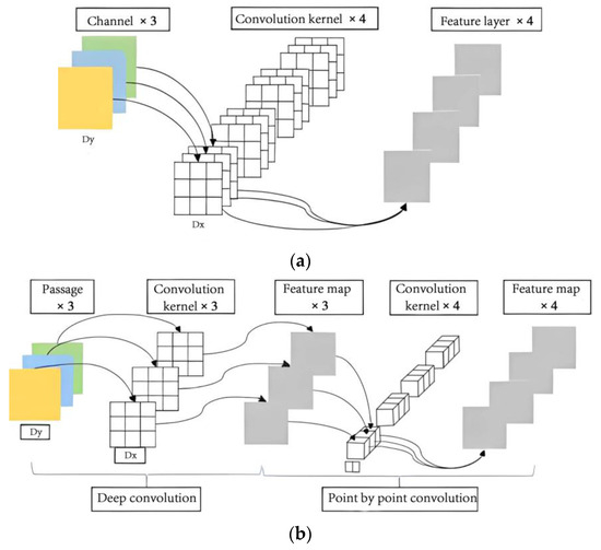
Figure 2.
The structural framework of deep learning systems. (a) Traditional convolutional structure; (b) deep separable convolutional structure.
If the size of the input feature is DF × DF × M, the size of traditional convolutional kernels is DK × DK × M × N. M and N refer to the numbers of input and output channels, respectively. The output feature map size of traditional convolution is DF × DF × N. The calculation amount (T1) is
But for the deep separable convolution, under the same input feature, the size of the deep convolution kernel is DK × DK × 1 × M, and the size of the point-by-point convolution kernel is 1 × 1 × M × N. The dimensions of the output features corresponding to the two convolution processes are: DF × DF × M and DF × DF × N. Therefore, the calculation amount (T2) will be
Consequently, compared to traditional convolution, it is found that the proportion of computational workload for deep separable convolutions is
When the size of the convolutional kernel is 3 × 3, the computation compression amount is about 9 times, indicating that deep separable convolution is an effective lightweight network design method that can accelerate the training speed of the network.
Of course, deep separable convolution is also an effective feature extraction method. For example, when we consider the introduction of an inverse residual module [20], its structure is shown in Figure 3.
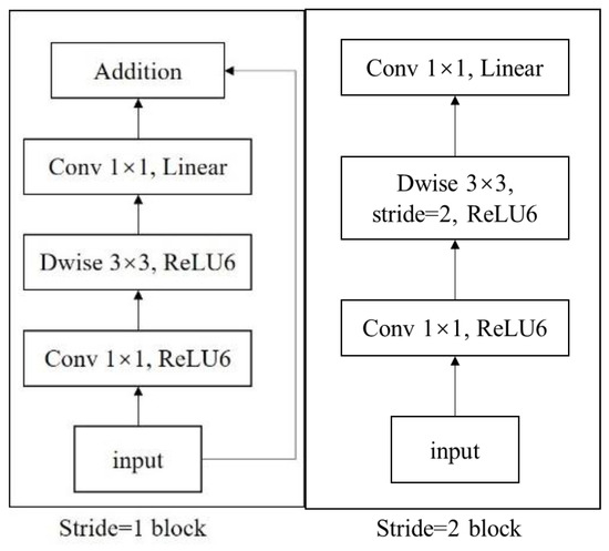
Figure 3.
Inverted residual structure module.
In Figure 3, only Stride = 1 block is used as an example for illustration. It can be found that this structure has three convolutional layers. The first one is 1 × 1 convolution, which is used to increase the dimensionality of input features. The second is 3 × 3 deep convolutions, and the third is 1 × 1 convolution. They form a deep separable convolution part, mainly responsible for feature extraction and dimensionality reduction of the output of the first convolution, and finally, adding the results and the original input through skip connections. The inverted residual structure is characterized by increasing the receptive field of the feature map through dimension increase, so that the deep separable convolution can learn more comprehensive feature representations. Compared to traditional convolution, this structure can flexibly adjust dimensions and more effectively reduce the computational complexity of the network.
The MobileNetv3 [21] network is a more efficient deep learning model. It takes advantage of the deep separable convolution and inverse residual structure, and the h-swish activation function is introduced. In this way, while reducing the computational load of the model, the added nonlinear layer in the inverse residual structure can be utilized to improve the fitting ability for nonlinear tasks. The h-swish activation function is simplified based on the swish function, and its expression is as follows:
wherein
The purpose of this study was to design a lightweight model to detect different types of malformed potatoes. Accordingly, the basic information of the backbone network, extracted by combining the advantages of Mobilenetv3 with the YOLOv3 framework, is shown in Table 1.

Table 1.
Improved feature extraction backbone network.
Table 1 shows the structure of the improved feature extraction backbone network. The third column represents the number of channels in the input feature layer of each bneck structure. X1, X2, and X3 represent feature maps of different scales output by the backbone network, respectively. In the backbone network, only the first and last layers use ordinary convolution, while the remaining layers are feature levels composed of multiple bneck structures. This model maintains high detection accuracy while reducing the calculation workload.
2.3. Test Environment and Evaluation Indicators
The environment for all tests in this paper is as follows: 64 bit Windows 10 operating system, x64 processor (Core i5-4570, Intel (China), Shanghai, China, 3.2 GHz), 8G running memory, AMD Radeon HD 8470 graphics card, PyCharm 2021.1.3 programming language, and TensorFlow deep learning framework. In order to evaluate the quality of the test results, this paper mainly uses the following four indicators: precision (P), recall (R), and mean average precision (mAP). The calculation formula is as follows:
In Equations (14)–(16) above, TP, FP, and FN are the correct number, error number, and missed number during the algorithm detection, respectively; N is the total number of categories detected by the algorithm.
3. Data and Analysis
3.1. Overview of Test Design
In order to evaluate the improvement effect of the YOLOv3 algorithm, different evaluation indicators described in this article were used to compare the performance of the algorithm before and after the improvement. Since the theoretical basis of the algorithm in this study has already been stated, this section first introduces the preparation of the dataset and elaborates on the changes in various evaluation indicators during the training process of the improved YOLOv3 model. Then, through ablation tests and horizontal comparisons, the superiority of the improved algorithm is further displayed. More importantly, in order to illustrate the progress of the new algorithm from both the details and the overall perspective, a comparison between AP and mAP is made. Finally, through the comparison of visual results, the application value of this research is more intuitively demonstrated.
3.2. Dataset Preparation
There is also a very important issue that needs to be explored here, which is the basic concept of potato malformation. There is no standard definition for potato malformation. However, in general, according to the basic characteristics of the appearance of most potatoes and the actual demand for commercialization, potatoes with a nearly circular or elliptical shape, and a relatively flat and regular surface, are considered normal potatoes (as shown in Figure 4a), while common malformations include local protrusion (as shown in Figure 4b), local depression (as shown in Figure 4c), proportional imbalance (as shown in Figure 4d), and mechanical injury (as shown in Figure 4e).
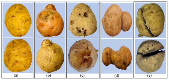
Figure 4.
Typical samples of potatoes. (a) Normal potatoes; (b) local protrusion; (c) local depression; (d) proportional imbalance; (e) mechanical injury.
The test dataset of this paper was collected from Longshu-9 and Longshu-10, planted in Majie Town, Wudu District, Longnan City, Gansu Province (1244 m ALT). The potato images were captured using a Canon EOS R6 micro single camera with 20 million pixels and a continuous shooting speed of 12 images per second at a fixed angle and distance. Among them, 2648 photos were taken with Longshu-9 and 1189 with Longshu-10. A total of 3837 photos of potatoes were collected, including 1950 photos of normal potatoes and 1887 photos of malformed potatoes. Among the malformed potatoes, 490 had a local protrusion, 480 had a local depression, 478 had a proportional imbalance, and 439 had a mechanical injury.
All the pictures were sized to 416 × 416 pixels, and the collected pictures were marked with the Labelimg tool. The format of each potato picture was originally xml; the xml was converted into a txt file using code, and the potato category and position coordinates were saved in the txt file. Then, we used VOC to create a dataset of potato images with different appearance features, and we configured the model environment so that the images could be trained in the model. Finally, all the marked pictures were divided into a training set, actual test set, and verification set; the dataset information is shown in Table 2.
Table 2.
Dataset information.
3.3. Network Training
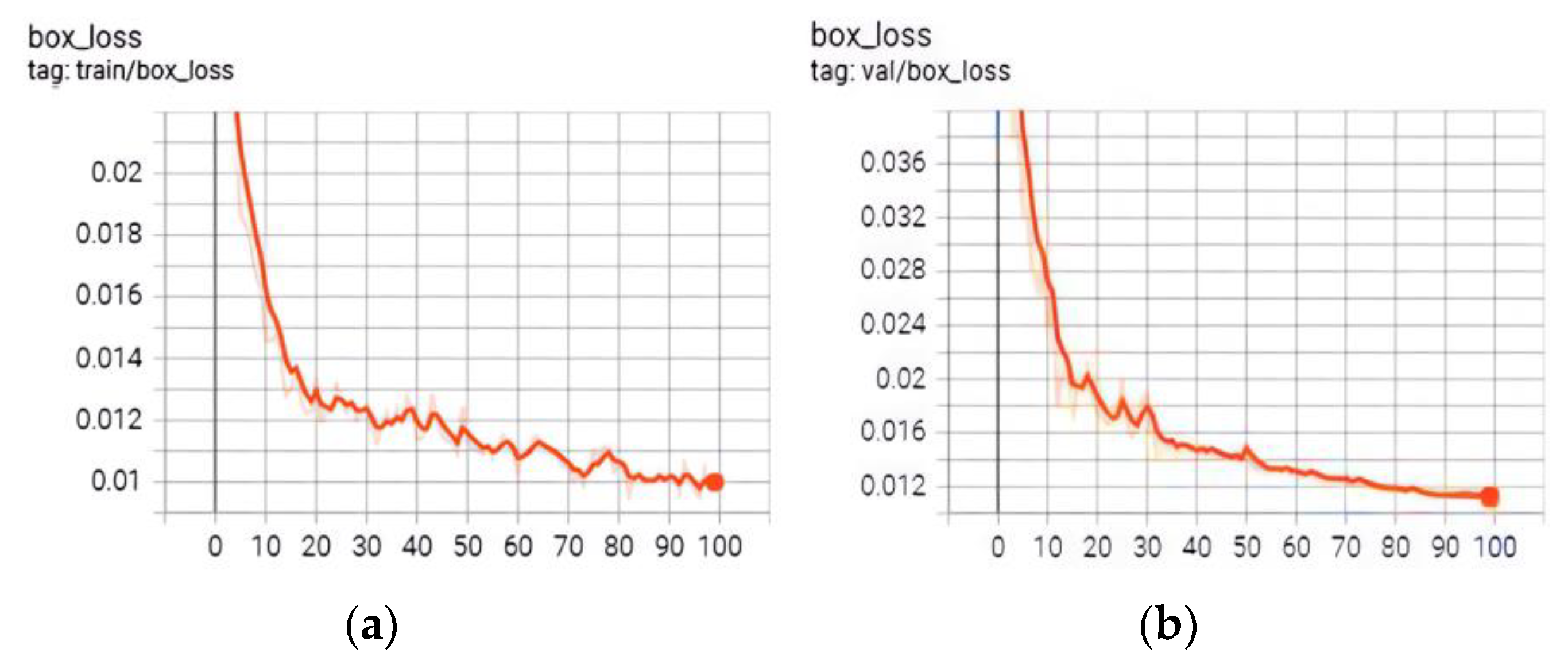
To understand the comparative performance of the improved YOLOv3 network, it was necessary to train the original network using the same dataset images. During the training process, the following parameter settings were followed: batch size was 2, initial learning rate was 0.01, momentum was 0.9, and the number of training rounds was 100. The change curves of the training loss function of the YOLOv3 network before and after the improvement are shown in Figure 5, where the horizontal coordinate system is the number of training rounds and the vertical is the loss. According to Figure 5, it can be found that the loss function of the algorithm before and after the improvement showed a downward tendency in the training process, which indicated that the training was successful, the network was convergent, and further in-depth testing could be carried out. However, the difference between the two curves in Figure 5 is also evident. Because the MSE loss function in target box regression is used in the basic YOLOv3 algorithm, it is sensitive to outliers with large errors, which easily cause regression divergence. It is obvious that the curve in Figure 5a has significant local fluctuations and relatively prominent instability. But the curve in Figure 5b is relatively smooth. This is precisely because the improved YOLOv3 algorithm uses CIOU as the regression loss function, which significantly suppresses the original local severe oscillation. The change in external loss indicators is an external manifestation of the internal stability; therefore, the improved algorithm had better convergence characteristics than before.
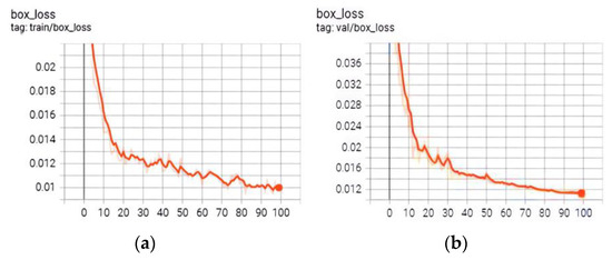
Figure 5.
Loss function curve. (a) Before improvement (performance of MSE); (b) after improvement (performance of CIOU).
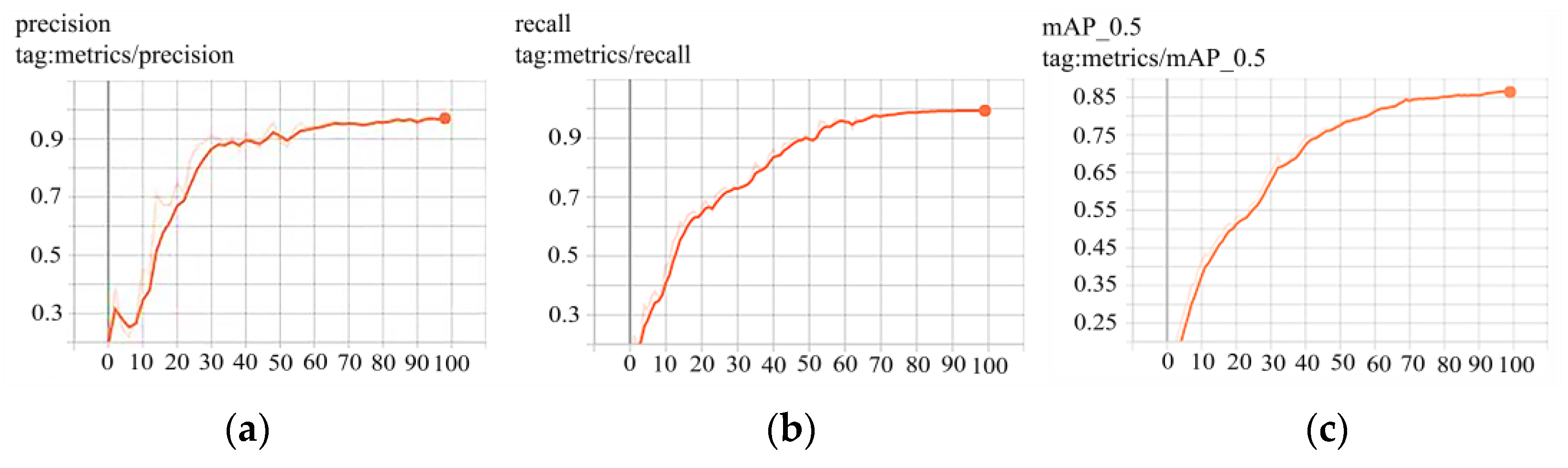
The improved YOLOv3 algorithm was trained on the obtained dataset, and the training process and various parameter indicators are shown in Figure 6. In the first 30 rounds of the training process, P increased rapidly, and then the ascent speed gradually slowed, while R and mAP increased relatively slowly. When the training reached 50 rounds, P gradually stabilized, while R and mAP continued to rise. When the training reached 80 rounds, the R, P, and mAP curves all tended to be stable, indicating that the model training process was almost over. The variation results of the parameters shown in Figure 6 indicated that the improved YOLOv3 model trained based on the training set was successful; moreover, the results of the verification set also showed that the parameter selection for this model training was reasonable. Its specific quantitative and qualitative advantages still needed to be tested, and the results of that work are presented below.
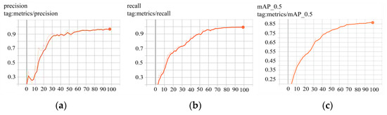
Figure 6.
Changes in main parameter indicators during the improved algorithm training process. (a) Precision (P); (b) recall (R); (c) main average precision (mAP).
3.4. Test Data and Analysis
3.4.1. Ablation Test
To achieve higher-performance algorithms for detecting different types of malformed potatoes, CIOU loss was used to replace MSE in the YOLOv3 algorithm (Algorithm Improvement 1). Then, deep separable convolution was used to replace the traditional convolution (Algorithm Improvement 2). Two methods were combined to improve the YOLOv3 algorithm. An ablation test was performed on the improved algorithm, and then the performance indicators of the algorithm before and after improvement were compared. The improvement effect of the algorithm in terms of memory capacity and mAP is shown in Table 3.
Table 3.
Comparison of performance indicators before and after the algorithm improvement.
The information in Table 3 shows that, in the YOLOv3 algorithm transformation, only separable convolutions are used to replace traditional convolutions, which can significantly reduce the model’s storage capacity from 59.85 M to 19.55 M, while mAP only slightly increases by 0.88%. Therefore, the main effect of Algorithm Improvement 1 lies in the model’s light weight. However, when replacing MSE with CIOU loss alone, the model’s storage capacity remains largely unchanged, but mAP significantly increases by 4.44%. As a consequence, the actual performance of Algorithm Improvement 2 lies in the enhancement of model identification ability.
After the two methods were integrated and the model’s training had been completed, the storage space of the improved YOLOv3 algorithm was 20.43 M, which was reduced by nearly 66% compared with the original, and the mAP could be 93.11%. This indicated that, after combining these two improved algorithms, their respective original advantages had been basically inherited, which made the improved YOLOv3 algorithm not only lightweight, but also gave it higher recognition and meant it could distinguish more subtle sample differences.
3.4.2. Horizontal Comparison Test
In order to test the relative effectiveness of the improved algorithm, the SSD, YOLOv3-Tiny, Faster R-CNN, YOLOv3 algorithm, and the improved YOLOv3 algorithm were trained using the same dataset and tested under the same epochs, confidence level, and initial learning rate. The comparative data of the results of the above five algorithms are shown in Table 4.
Table 4.
Comparison of different algorithms.
Table 4 shows that, among the five network models compared, although the improved YOLOv3 algorithm is not excellent in detection time, it has significant advantages in crucial training time and memory capacity. This indicates that, compared to the mainstream algorithms in this field, the YOLOv3 model improvement scheme described in this study has outstanding effectiveness, meaning it is more suitable for application deployment using lightweight devices.
3.4.3. Comparison of AP and mAP
In order to quantitatively verify the performance of the improved YOLOv3 algorithm, the dataset in this paper was used for training, and weights of the same confidence were set for testing. In this section, AP and mAP values of SSD, YOLOv3, YOLOv3-TINY, Faster R-CNN, and the improved YOLOv3 algorithm are compared. The test results are shown in Table 5.
Table 5.
Comparison of AP and mAP values for different algorithms.
The data in Table 5 show that the improved YOLOv3 algorithm proposed in this article has a mAP of 93.11%, which is increased by 6.79%, 4.68%, and 9.16% compared to the SSD, YOLOv3, and Faster R-CNN algorithms, respectively. Compared to the lightweight algorithm YOLOv3-Tiny, it is increased by 7.27%, and the AP values of each class have been improved to varying degrees compared to the other algorithms. This indicates that the use of the improved backbone feature extraction network and CIOU regression optimization loss function improves the detection performance of the model, leading it to show significant advantages.
3.4.4. Comparison of Visualization Results
In order to demonstrate whether the improved algorithm had missed or falsely detected results an, visualization tests were conducted on different types of potato combinations, such as a single malformed potato with a normal potato, any combination of two different kinds of malformed potatoes, or several different kinds of malformed potatoes with a normal potato.
Due to the obvious difference in potato shape of a single malformed potato when compared to a normal potato, and since we made arbitrary combinations of two different types of malformed potatoes, because different types of potatoes could be correctly identified in all such test samples, the detection results before and after the algorithm improvement were not necessarily compared one by one. Accordingly, only the typical schematic diagrams of the improved algorithm’s detection results are shown in Figure 7, Figure 8 and Figure 9. However, for the combinations of multiple malformed potatoes with a normal potato, there were many potato shapes involved, and there were stacked, overlapped, and scattered images to be tested. The potato shapes in the diagram were complex and diverse, so a comparison of the detection schematic diagrams before and after the improvement is presented separately (Figure 10).
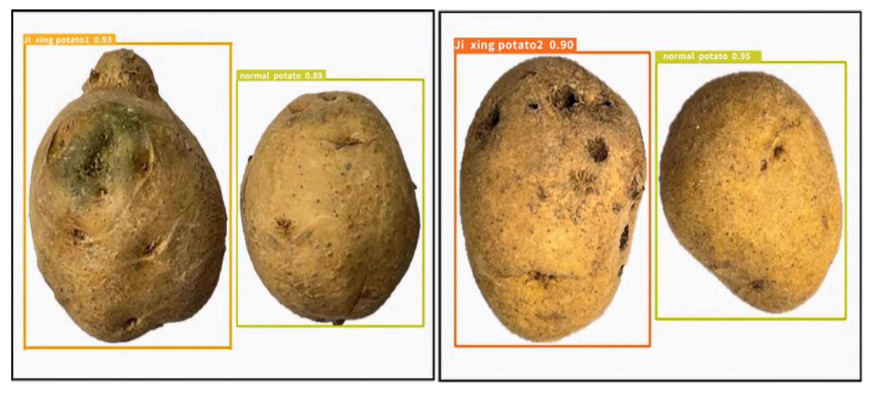
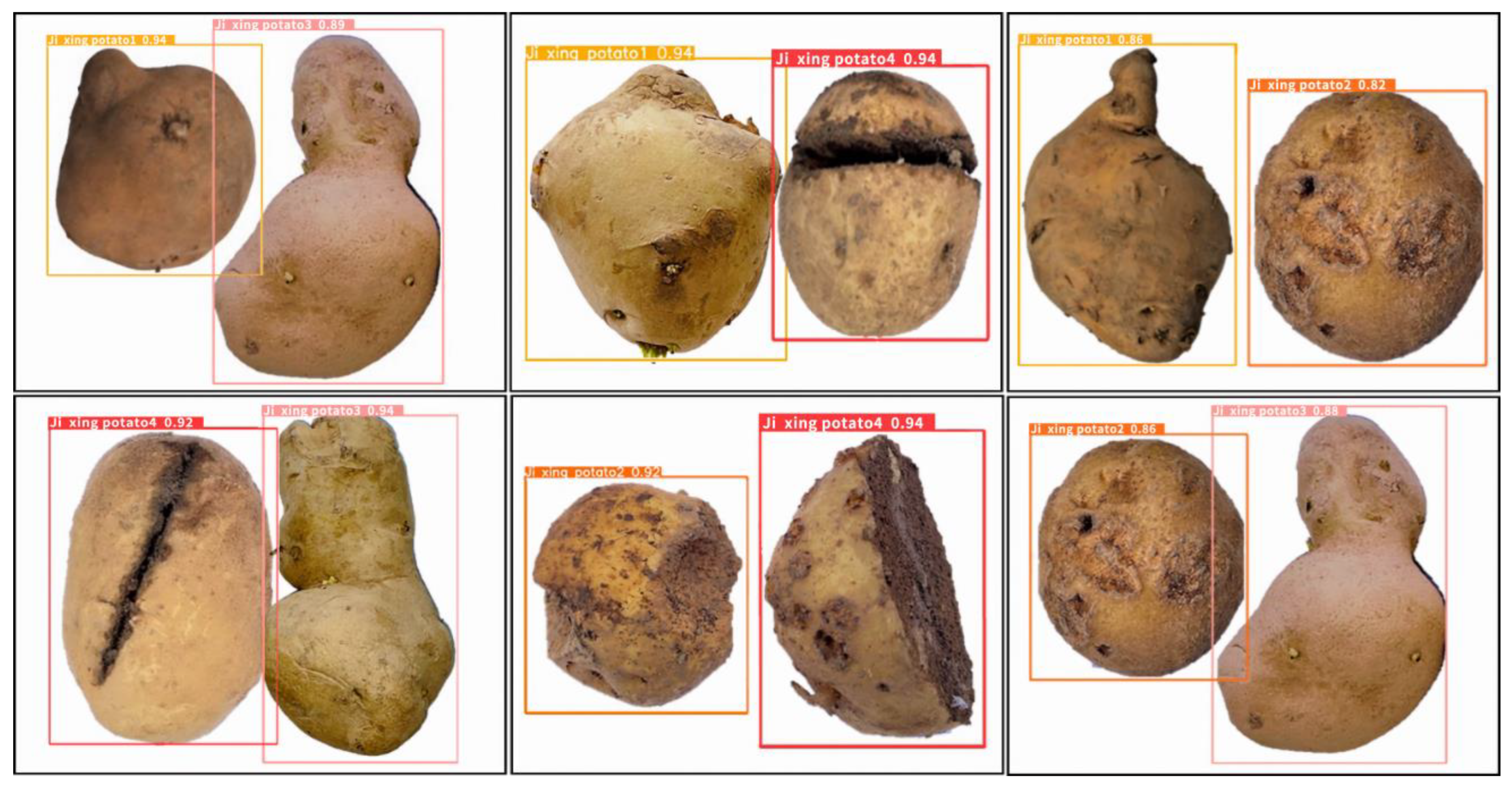
Figure 7, Figure 8 and Figure 9 correspond to the recognition results of a single malformed potato, the combination of a single malformed potato with a normal potato, the arbitrary combination of two different types of malformed potatoes, and different kinds of malformed potatoes with a normal potato. To distinguish different potato shapes, different labels were given for the detection images: “normal potato” for normal potatoes; the locally protruding malformed potato was labeled “Ji Xing potato1”; the locally depressed malformed potato was labeled “Ji Xing potato2”; the proportion-imbalance-malformed potato was labeled “Ji Xing potato3”; and the malformed potato with mechanical damage was classified as “Ji Xing potato4”.
- (1)
- Single malformed potato
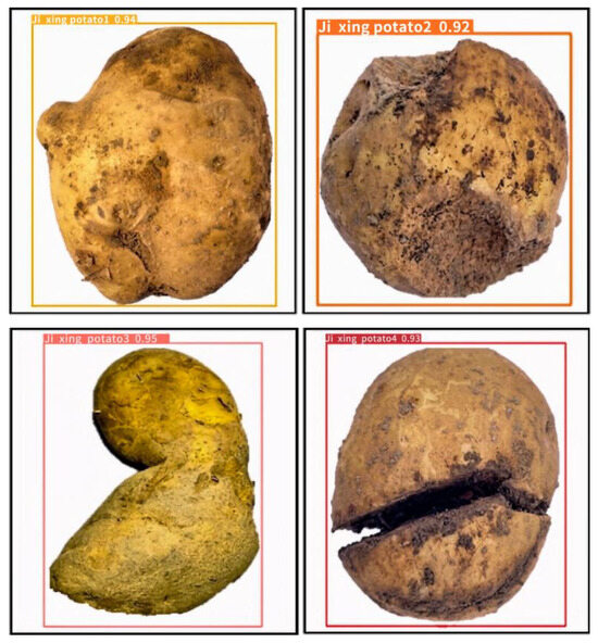
Figure 7.
Detection results of single malformed potato (Improved YOLOv3).
Figure 7.
Detection results of single malformed potato (Improved YOLOv3).

- (2)
- Single malformed potato and a normal potato

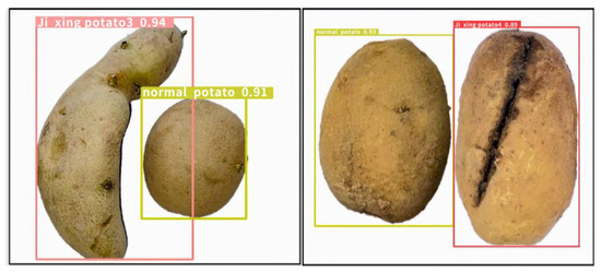
Figure 8.
Detection results of single malformed potato and a normal potato (Improved YOLOv3).
Figure 8.
Detection results of single malformed potato and a normal potato (Improved YOLOv3).

- (3)
- Two different types of malformed potatoes
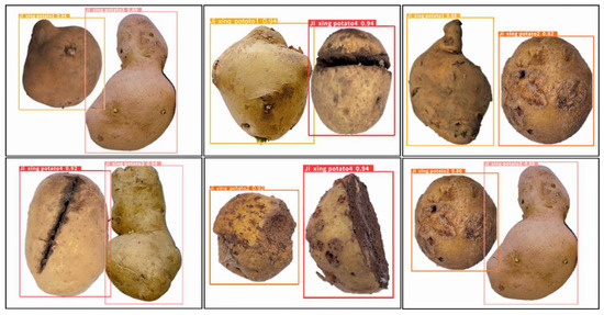
Figure 9.
Detection results of two different types of malformed potatoes (Improved YOLOv3).
Figure 9.
Detection results of two different types of malformed potatoes (Improved YOLOv3).
- (4)
- Different kinds of malformed potatoes and a normal potato
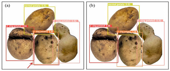
Figure 10.
Detection results of different types of malformed potatoes and one normal potato. (a) One local depression was recognized falsely (Original YOLOv3); (b) local depression was recognized correctly (Improved YOLOv3).
Figure 10.
Detection results of different types of malformed potatoes and one normal potato. (a) One local depression was recognized falsely (Original YOLOv3); (b) local depression was recognized correctly (Improved YOLOv3).

The test set shown in Table 2 or its necessary combinations were used to form the required test set for this next step, by which means we generated the required complex test scenarios in the most economical and efficient way. The detection results in Figure 7, Figure 8 and Figure 9 show that most potatoes could be reliably identified with an accuracy rate of no less than 95%. However, Figure 10 shows the detection results of different kinds of malformed potatoes with a normal potato. Among them, Figure 10a is the detection results of the original YOLOv3 model, while Figure 10b is the outcome of the improved algorithm. In Figure 10a, there is a combination of local depression, proportional imbalance, mechanical injury, and normal potatoes, which are stacked and partially overlapped. In this picture, a local depression malformed potato is falsely detected and has obvious double boxes, which have been marked with red arrows. However, based on the improved YOLOv3 proposed in this study, the identification results of the same image are accurate, without any mistake (see Figure 10b).
In order to verify the feasibility of the improved YOLOv3 algorithm in complex situations on a larger scale, a total of 180 multi-shape mixed-potato photos were used for recognition, and the results are shown in Table 6. The information displayed in Table 6 indicates that the original YOLOv3 had a correct detection count of 160, missed detection of 2, and false detections of 18. However, the improved algorithm had a detection count of 167, missed detection of 1, and false detections of 12. Therefore, according to Figure 10 and Table 6, the improved YOLOv3 algorithm performed better in detection.
Table 6.
Statistics of potato malformation detection using different algorithms.
4. Conclusions
- (1)
- In terms of feature extraction backbone networks, deep separable convolution was adopted to fuse features at various scales, which not only greatly reduced the storage space requirements of the model but also helped to improve detection accuracy.
- (2)
- In terms of target box regression, CIOU loss was adopted, and the problem of unstable and inequivalent target box regression caused by MSE loss was solved. This not only ensures the diversity of extractable features but also significantly improves the detection accuracy without increasing the model storage capacity.
- (3)
- Compared with the original algorithm, the improved YOLOv3 made mAP increase by 4.68%, 6.1 h training time was saved, and the storage capacity of the model reduced by approximately 66%. Specifically, the AP values of local protrusion, local depression, proportion imbalance, and mechanical injury of the improved algorithm were 94.13%, 91.00%, 95.52%, and 91.79%, respectively. Those had all progressed significantly compared to before the improvement, and the comparison of visualization results also confirmed the effectiveness of the improved algorithm in this paper.
5. Discussion
This study adopted the above improvement methods. Although there was gratifying progress in the fine classification of potato malformations, further attention should be paid to the following aspects:
- (1)
- The definition of a malformed potato in this study was not sufficiently standardized, making it difficult to distinguish some malformed potatoes that were not particularly obvious during training of this system. Therefore, it is necessary to provide a clearer definition of the concept of potato appearance malformations, and if necessary, these should be treated differently according to the variety.
- (2)
- In the feature-fusion output-channel-improved YOLOv3 algorithm, the improved the output channel was still quite traditional; other methods can be adopted to make more effective improvements in the future.
- (3)
- This study had limited classification of malformations; for example, these can also include malformations caused by surface diseases or local or large-scale epidermal attachments. Therefore, the recognition and classification of malformations in this system is not sufficient. In future research, higher-level networks and more systematic partitioning can be used to achieve more effective classification.
Author Contributions
Conceptualization, G.W., W.Y. and W.S.; methodology, G.W. and Q.W.; software, Q.W. and S.Y.; validation, G.W., Q.W. and H.L.; formal analysis, G.W. and W.S.; investigation, X.Y.; resources, Q.W. and Y.L.; data curation, Y.L.; writing—original draft preparation, G.W., Y.L. and Q.W.; writing—review and editing, G.W., Y.L. and Q.W.; visualization, B.F.; supervision, G.W.; funding acquisition, G.W., W.Y., W.S. and S.Y. All authors have read and agreed to the published version of the manuscript.
Funding
This research was funded by the Industrial Support Plan (Education Department of Gansu Province, 2023CYZC-42); the Young PhD Fund Project (Education Department of Gansu Province, 2021QB-033); the National Natural Science Foundation of China (NSFC, 52165028, 32201663); and the Key Scientific and Technological Program of Gansu Province (Science and Technology Department of Gansu Province, 22ZD6NA046).
Data Availability Statement
Not applicable.
Conflicts of Interest
The authors declare no conflict of interest.
References
- Zhang, H.; Xu, F.; Wu, Y.; Hu, H.H.; Dai, X.F. Progress of potato staple food research and industry development in China. J. Integr. Agric. 2017, 16, 2924–2932. [Google Scholar] [CrossRef]
- Scarpa, F.; Colonna, A.; Ruggeri, A. Multiple-image deep learning analysis for neuropathy detection in corneal nerve images. Cornea 2020, 39, 342–347. [Google Scholar] [CrossRef] [PubMed]
- Muhammad, U. Research on the Method of Judging Litchi Maturity and Size Based on Image Deep Learning. Master’s Thesis, South China University of Technology, Guangzhou, China, 8 June 2020. [Google Scholar]
- Shahbaz, K.; Muhammad, T.; Muhammad, T.K.; Zubair, A.K.; Shahzad, A. Deep learning-based identification system of weeds and crops in strawberry and pea fields for a precision agriculture sprayer. Precis. Agric. 2021, 22, 1711–1727. [Google Scholar]
- Kermany, D.S.; Goldbaum, M.; Cai, W.; Valentim, C.C.S.; Liang, H.; Baxter, S.L.; Mckeown, A.; Ge, Y.; Wu, X.; Yan, F. Identifying medical diagnoses and treatable diseases by image-based deep learning. Cell 2018, 172, 1122–1131. [Google Scholar] [CrossRef] [PubMed]
- Casado-García, A.; Heras, J.; Milella, A.; Marani, R. Semi-supervised deep learning and low-cost cameras for the semantic segmentation of natural images in viticulture. Precis. Agric. 2022, 23, 2001–2026. [Google Scholar] [CrossRef]
- Harmandeep, S.G.; Osamah, I.K.; Youseef, A.; Saleh, A.; Fawaz, A. Fruit image classification using deep learning. Comput. Mater. Contin. 2022, 71, 5135–5150. [Google Scholar]
- Erwin, A.D.; Suprihatin, B.; Agustina, S.B. A robust techniques of enhancement and segmentation blood vessels in retinal image using deep learning. Biomed. Eng. Appl. Basis Commun. 2022, 34, 2250019. [Google Scholar]
- Bian, B.C.; Chen, T.; Wu, R.J.; Liu, J. Improved YOLOv3-based defect detection algorithm for printed circuit board. J. Zhejiang Univ. (Eng. Sci.) 2023, 57, 735–743. (In Chinese) [Google Scholar]
- Li, Z.H.; Zhang, L. Safety helmet wearing detection method of improved YOLOv3. Foreign Electron. Meas. Technol. 2022, 41, 148–155. (In Chinese) [Google Scholar]
- Qin, W.W.; Song, T.N.; Liu, J.Y.; Wang, H.W.; Liang, Z. Remote sensing military target detection algorithm based on lightweight YOLOv3. Comput. Eng. Appl. 2021, 57, 263–269. (In Chinese) [Google Scholar]
- Zhang, B.; Xu, F.; Li, X.T.; Zhao, Y.D. Research on the improved YOLOv3 algorithm for military cluster targets. Fire Control Command Control 2021, 46, 81–85. (In Chinese) [Google Scholar]
- Chen, N.; Feng, Z.; Li, F.; Wang, H.; Yu, R.; Jiang, J.; Tang, L.; Rong, P.; Wang, W. A fully automatic target detection and quantification strategy based on object detection convolutional neural network YOLOv3 for one-step X-ray image grading. Anal. Methods 2023, 15, 164–170. [Google Scholar] [CrossRef] [PubMed]
- Zhang, Z.; Zhang, Y.; Wen, Y.; Fu, K.; Luo, X.Y. Intelligent defect detection method for additive manufactured lattice structures based on a modified YOLOv3 model. J. Nondestruct. Eval. 2022, 41, 3. [Google Scholar] [CrossRef]
- Temniranrat, P.; Kiratiratanapruk, K.; Kitvimonrat, A.; Sinthupinyo, W.; Patarapuwadol, S. A system for automatic rice disease detection from rice paddy images serviced via a Chatbot. Comput. Electron. Agric. 2021, 185, 106156. [Google Scholar] [CrossRef]
- Tassis, L.M.; de Souza, J.E.T.; Krohling, R.A. A deep learning approach combining instance and semantic segmentation to identify diseases and pests of coffee leaves from in-field images. Comput. Electron. Agric. 2021, 186, 106191. [Google Scholar] [CrossRef]
- Redmon, J.; Farhadi, A. YOLOv3: An Incremental Improvement. arXiv 2018, arXiv:1804.02767. [Google Scholar]
- Gong, C.; Li, A.; Song, Y.; Xu, N.; He, W. Traffic sign recognition based on the YOLOv3 algorithm. Sensors 2022, 22, 9345. [Google Scholar] [CrossRef] [PubMed]
- Zheng, Z.; Wang, P.; Liu, W.; Li, J.; Ye, R.; Ren, D. Distance-IoU loss: Faster and better learning for bounding box regression. In Proceedings of the Thirty-Fourth AAAI Conference on Artifieial Inelligence, New York, NY, USA, 7–12 February 2020. [Google Scholar]
- Sandler, M.; Howard, A.; Zhu, M.; Zhmoginov, A.; Chen, L.C. Mobilenetv2: Inverted residuals and linear bottlenecks. In Proceedings of the IEEE Conference on Computer Vision and Pattern Recognition, Salt Lake City, UT, USA, 18–22 June 2018. [Google Scholar]
- Howard, A.; Sandler, M.; Chu, G.; Chen, L.C.; Chen, B.; Tan, M.; Wang, W.; Zhu, Y.; Pang, R.; Vasudevan, V.; et al. Searching for mobilenetv3. In Proceedings of the International Conference on Computer Vision 2019, Seoul, Republic of Korea, 27 October–2 November 2019. [Google Scholar]


Disclaimer/Publisher’s Note: The statements, opinions and data contained in all publications are solely those of the individual author(s) and contributor(s) and not of MDPI and/or the editor(s). MDPI and/or the editor(s) disclaim responsibility for any injury to people or property resulting from any ideas, methods, instructions or products referred to in the content. |
© 2023 by the authors. Licensee MDPI, Basel, Switzerland. This article is an open access article distributed under the terms and conditions of the Creative Commons Attribution (CC BY) license (https://creativecommons.org/licenses/by/4.0/).