Enhancing Swarm Intelligence for Obstacle Avoidance with Multi-Strategy and Improved Dung Beetle Optimization Algorithm in Mobile Robot Navigation

Abstract

The Dung Beetle Optimization (DBO) algorithm is a powerful metaheuristic algorithm that is widely used for optimization problems. However, the DBO algorithm has limitations in balancing global exploration and local exploitation capabilities, often leading to getting stuck in local optima. To overcome these limitations and address global optimization problems, this study introduces the Multi-Strategy and Improved DBO (MSIDBO) Algorithm. The MSIDBO algorithm incorporates several advanced computational techniques to enhance its performance. Firstly, it introduces a random reverse learning strategy to improve population diversity and mitigate early convergence or local stagnation issues present in the DBO algorithm. Additionally, a fitness-distance balancing strategy is employed to better manage the trade-off between diversity and convergence within the population. Furthermore, the algorithm utilizes a spiral foraging strategy to enhance precision, promote strong exploratory capabilities, and prevent being trapped in local optima. To further enhance the global search ability and particle utilization of the MSIDBO algorithm, it combines the Optimal Dimension-Wise Gaussian Mutation strategy. By minimizing premature convergence, population diversity is increased, and the convergence of the algorithm is accelerated. This expansion of the search space reduces the likelihood of being trapped in local optima during the evolutionary process. To demonstrate the effectiveness of the MSIDBO algorithm, extensive experiments are conducted using benchmark test functions, comparing its performance against other well-known metaheuristic algorithms. The results highlight the feasibility and superiority of MSIDBO in solving optimization problems. Moreover, the MSIDBO algorithm is applied to path planning simulation experiments to showcase its practical application potential. A comparison with the DBO algorithm shows that MSIDBO generates shorter and faster paths, effectively addressing real-world application problems.

1. Introduction

Mobile robots have demonstrated their success in various fields such as industries, military operations, and search and rescue missions, effectively carrying out critical unmanned tasks. In this highly intelligent and modern society, path planning plays a vital role in enabling these mobile robots to navigate and explore complex environments [1,2]. The objective of path planning is to find an optimal or suboptimal path from the initial state to the target state, considering specific performance criteria and the characteristics of the robot and its working environment [3,4].

Traditional path planning approaches have been investigated extensively. For instance, Yao et al. [5] proposed an improved artificial potential field method to address the problem of this technique falling into trap areas and local minima during the planning process. Experimental results demonstrated that the enhanced algorithm effectively overcomes these issues. Kandathil et al. [6] implemented the BUG-1 algorithm across a group of robots to move them from a start location to a target location, significantly reducing the time required for robot movement. Huang et al. [7] introduced a novel approach called the navigation strategy with path priority (NSPP) for multiple robots moving within a large flat space. NSPP utilizes Voronoi diagrams to divide the map based on each robot’s path-priority order and performs path planning for the robots in the space. This method can be applied to any number of robots and exhibits superior performance in terms of average trajectory length. Alshammrei et al. [8] designed and practically implemented an optimal collision-free algorithm based on an improved Dijkstra algorithm. The results indicate that the enhanced Dijkstra algorithm efficiently solves the optimal path planning problem for mobile robots navigating through environments containing obstacles. Ma [9] proposed a bidirectional search Probabilistic Roadmaps global path planning algorithm to address the limitations of low search efficiency and excessive path turning points in Probabilistic Roadmaps. Simulation results demonstrate that the improved algorithm effectively improves convergence speed and path smoothness when applied in actual mobile robot navigation experiments. Kang [10] presented an enhanced rapidly-exploring random tree (RRT) algorithm to address the issues of low planning efficiency and unsmooth paths in complex environments. The simulation results indicate significantly improved planning efficiency and path smoothness for mobile robots. Wang et al. [11] proposed a road stiffness planning algorithm called NRRT* based on convolutional neural networks (CNN). This algorithm is capable of quickly obtaining high-quality paths and accelerating convergence speed. On the other hand, Chi et al. [12] proposed a heuristic path planning algorithm based on the Generalized Voronoi Graph (GVD). This algorithm has the ability to automatically recognize environmental features and provide reasonable heuristic paths.

It is evident that although traditional path planning algorithms possess numerous advantages, they often fail to provide globally optimal paths. Additionally, when confronted with complex environments, these methods exhibit high computational costs and low success rates, making it challenging to meet practical application requirements. As a result, researchers have turned their attention towards meta-heuristic path planning methods due to their distributed computing capabilities, independence from prior knowledge, and robustness. In recent years, significant research advancements have been made in the field of group intelligent optimization algorithms for path planning. For example, Pehlivanoglu et al. [13] proposed an initial population enhancement method in genetic algorithms, thereby accelerating convergence speed. Patle et al. [14] conducted research on classical and reactive methods and found that reactive methods are more robust. When used as a hybrid algorithm, reactive methods are used to improve the performance of classical methods. Mohanty Prases et al. [15] proposed a smart adaptive particle swarm optimization algorithm for robot path planning. This algorithm enables robots to reach target points by using the shortest possible paths while safely avoiding obstacles in uncertain environments. Wu et al. [16] introduced an improved ant colony optimization algorithm to enhance convergence speed and global optimization effects. Simulation results demonstrate the effectiveness and efficiency of this algorithm in solving path planning problems for mobile robots within various constraint environments. Ge et al. [17] proposed an improved A* algorithm that considers energy consumption for path planning of spherical robots. The results indicate that compared to traditional path planning algorithms, the proposed method minimizes energy consumption and path length for spherical robots as much as possible. Zhang et al. [18] improved the sparrow search algorithm by introducing a fitness-distance balance and integrating the Harris Hawks algorithm. These enhancements aimed to overcome issues related to premature convergence and a decline in population diversity observed in the basic sparrow search algorithm.

Guo et al. [19] developed a multistrategy improved whale optimization algorithm specifically for trajectory planning of upper extremity exoskeleton rehabilitation robots, focusing on isokinetic rehabilitation. This algorithm provides a feasible solution for isokinetic rehabilitation trajectory planning of upper extremity exoskeleton rehabilitation robots. Gao et al. [20] presented a novel robot path planning algorithm based on Quantum-inspired Evolutionary Algorithm. Simulation results indicate that this algorithm is suitable for both complex static and dynamic environments and outperforms conventional genetic algorithms in solving robot path planning problems by effectively optimizing the paths. Zhang et al. [18] enhanced the sparrow search algorithm by incorporating fitness-distance balance and the Harris Hawks algorithm to address issues such as premature convergence and declining population diversity. Simulation experiments conducted in unknown environments demonstrate the effectiveness and robustness of the proposed algorithm in solving local path planning problems for mobile robots. Hong Kwon Ryong et al. [21] proposed an algorithm called Rao-combined artificial bee colony for designing minimum path planning to minimize radiation exposure to nuclear power plant workers. The experimental results reveal that the proposed method surpasses traditional algorithms in terms of exploration, exploitation, convergence, and robustness. Li et al. [22] aimed to enhance the sand cat swarm optimization algorithm for robot path planning by stochastic variation with elite collaboration. The results demonstrated the effectiveness and engineering practicability of the improved algorithm in addressing the path planning problem for mobile robots. The work proposed by Jiang et al. [23] is significant as it addresses the challenge of navigating complex environments effectively. By incorporating SLAM, tracking, and detection methods, their framework offers a comprehensive solution of robust and reliable localization in multi-story buildings. Dong et al. [24] introduced an improved grey wolf optimization algorithm that overcomes issues related to premature convergence and falling into local optima. The experimental results indicate that this optimization outperforms other competitors and its applicability is verified through a robot global path planning problem, demonstrating its ability to plan shorter and safer paths. Li et al. [25] proposed an improved multiobjective genetic algorithm for solving static global path planning. Simulation experiments conducted in grid environments demonstrate that the algorithm addresses issues present in traditional genetic algorithms, such as slow convergence speed and susceptibility to local optima.

The DBO algorithm is a novel swarm intelligence algorithm inspired by the rolling, dancing, foraging, stealing, and reproduction behaviors of dung beetles. The DBO algorithm exhibits strong optimization capabilities and fast convergence. However, it also suffers from limitations such as an imbalance between global exploration and local exploitation, a tendency to get trapped in local optima, and relatively weaker global exploration abilities. Many scholars have endeavored to optimize and improve this algorithm. Zhu et al. [26] proposed a dung beetle search algorithm called QHDBO that combines quantum computing and multi-strategy techniques. They utilized a good point set strategy to initialize the initial population of dung beetles, ensuring a more uniform distribution and reducing the likelihood of falling into local optima. QHDBO was compared with six other intelligent algorithms using 37 test functions and practical engineering application problems. The experimental results demonstrated that the optimized dung beetle optimization algorithm significantly improved convergence speed, optimization accuracy, and robustness. In a related study, Zhang et al. [27] introduced a modified mantis algorithm (IDBOP) to optimize a BP neural network for improving the prediction accuracy of wood mechanical behavior. They employed segmented linear chaos mapping to increase diversity and incorporated an adaptive parameter adjustment strategy to enhance early best search capabilities and improve search efficiency. Experimental results showed that optimizing the neural network model with IDBO greatly enhanced the prediction accuracy of wood mechanical properties. Building upon the improved sinusoid algorithm, Wang et al. [28] proposed an enhanced DBO algorithm called QQLDBO. This approach integrated quasi-oppositional learning and Q-learning, expanded the search scope, improved global exploration capabilities, and the variable spiral local domain method is proposed to make up for the shortage of developing only around the neighborhood optimum. The QQLDBO algorithm was tested using 23 benchmark test functions and compared with other well-known meta-heuristics, demonstrating its superior performance. Furthermore, the practical potential of the QQLDBO algorithm was validated by successfully applying it to engineering design problems, effectively addressing practical applications. Shen et al. [29] presented a multi-strategy enhancement of the dung beetle optimizer (MDBO) for drone (UAV) 3D path planning. They utilized Beta distribution to dynamically generate reflection solutions, allowing for exploration of a broader search space and enabling particles to escape local optima. Additionally, Levy distribution was introduced to handle bound particles, and two different cross operators were utilized to improve the thief beetle update stage. This strategy accelerated integration, balanced exploration, and development capabilities, and enhanced optimization accuracy and stability. MDBO’s effectiveness was confirmed through comparisons with other algorithms on benchmark functions. Moreover, the performance of MDBO in UAV 3D path planning was verified, successfully finding feasible paths even in challenging scenarios. The proposed MDBO algorithm demonstrated its capability to find safe and optimal paths in most cases, although it has limitations in avoiding local obstacles and may require multiple UAVs for complex situations.

Through previous research, researchers and practitioners can gain insight into the origins and development of the original algorithm, broaden their optimization approaches, integrate valuable strategies into their own to enhance existing technologies, and benefit from these discoveries. Building upon prior research, the MSIDBO algorithm addresses the issues of slow convergence speed, susceptibility to local optima, poor accuracy, and limited stability by incorporating approaches such as random reverse learning, fitness distance balance, spiral foraging, and optimal dimensional Gaussian mutation strategies. These improvements result in enhanced convergence speed and accuracy. The random reverse learning strategy enhances population diversity and alleviates the inherent challenges of premature convergence and local stagnation faced by the DBO algorithm. The fitness distance balance strategy effectively balances diversity and convergence within the population, mitigating between global exploration and local exploitation, which leads to inferior global search capabilities and vulnerability to local optima. Furthermore, the integration of the spiral foraging strategy improves search accuracy, demonstrating superior exploration capabilities and avoiding local optima. By combining the MSIDBO algorithm with the optimal dimensional Gaussian mutation strategy, premature convergence is reduced, global search capabilities are strengthened, particle utilization is improved, population diversity is increased, and the convergence speed of the MSIDBO algorithm is accelerated. This enables better escapement from local optima during the evolutionary process. It is evident that the proposed MSIDBO algorithm addresses the limitations and deficiencies of the original DBO algorithm. Researchers and practitioners can incorporate these strategies into their own or leverage specific aspects of the MSIDBO algorithm to enhance their existing techniques. It is worth noting that the aforementioned improvements are conducive to further advancements in the field and have the potential to significantly impact and improve existing algorithms. Additionally, 19 benchmark test functions are selected for simulation experiments, comparing the improved MSIDBO algorithm with the original DBO algorithm. The experimental results demonstrate that the improved algorithm not only generates relatively optimal paths but also significantly improves the speed of path planning. Moreover, as the size of the map increases, the effectiveness becomes more pronounced. The application of the improved algorithm in path planning experiments further confirms that MSIDBO can meet practical requirements, generating shorter and smoother paths with faster convergence. It exhibits high adaptability in complex environments and avoids various shaped obstacles, showcasing superior performance. By effectively utilizing the advantages of both global and local planning methods, it successfully resolves the problem of local obstacle avoidance when a global route has already been planned, thereby improving obstacle avoidance performance and ensuring globally optimal planned paths.

2. Methods

2.1. Dung Beetle Optimization (DBO) Algorithm

The DBO algorithm is a novel swarm intelligence optimization algorithm inspired by the social behavior of dung beetle populations. These beetles compress dung into balls before rolling them to a safe location. They can roll significantly larger dung balls and utilize celestial cues to roll them in a straight line when there is a light source available. However, in the absence of a light source, their paths become curved and susceptible to natural disturbances [30]. The survival of dung beetles is intricately linked to acquiring dung balls, where some are used for reproduction and nurturing offspring while the rest serve as food.

Motivated by this behavior, the DBO algorithm simulates five key behaviors exhibited by dung beetles: ball rolling, dancing, foraging, stealing, and reproduction. The dung beetle population is divided into four subgroups: rollers, reproducers, minors, and stealers, with different search strategies employed for each subgroup [31].

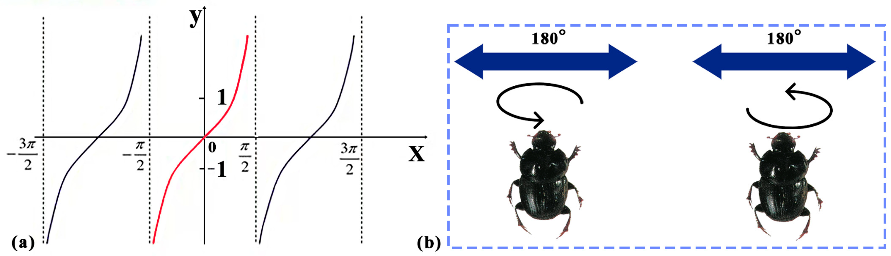
2.1.1. Roller Beetle

During the rolling process, dung beetles must navigate using celestial cues, particularly the sun, moon, and polarized light, to maintain the straight-line rolling trajectory of the dung ball. As shown in Figure 1, dung beetle trajectory model is displayed. It can be observed that dung beetles utilize the sun for navigation, with the arrow indicating the rolling direction [32].

Assuming that the intensity of the light source also influences the rolling path of dung beetles, the position of the roller beetle is updated and can be represented as follows [33]:

$$X_i(t+1)=X_i(t)+\alpha \times k\times X_i(t+1)+b\times \Delta x$$

(1)

$$\Delta x=\left|X_i(t)-X^w\right|$$

(2)

where t represents the current iteration count; X_i(t) represents the position information of the i-th dung beetle in the t-th iteration; k ∈ (0, 0.2] denotes a constant value indicating the deviation coefficient; b is a constant value belonging to the interval (0, 1); α is a natural coefficient assigned as either 1 or −1; X^w represents the global worst position; and ∆x simulates the variation of light intensity. The parameter a simulates natural factors (such as wind and uneven terrain) that can cause the dung beetle to deviate from its original direction. Specifically, a = 1 signifies no deviation, while a = −1 indicates deviation from the original direction. A larger ∆x implies weaker light source, which brings two benefits: (1) thoroughly exploring the entire problem space during the optimization process; (2) enhancing search capabilities and reducing the likelihood of getting trapped in local optima.

2.1.2. Dancing Behavior

Various natural factors, such as wind and uneven terrain, can have a significant impact on the trajectory of dung beetles. In such situations, dung beetles typically climb to the top of the dung ball and engage in a dancing behavior, which involves a series of rotations and pauses. Through this dancing behavior, they determine their movement direction by changing their orientation, thus obtaining a new path. To mimic this dancing behavior, a tangent function is employed to obtain the new rolling direction. Figure 2 shows the tangent function model and dancing model of dung beetles. It is important to note that only the values defined on the interval [0, 1] of the tangent function need to be considered, as shown in the diagram [34].

Once the correct direction is successfully determined, the roller beetle should continue rolling the ball forward. At this point, the position update of the roller beetle is as follows:

$$X_i(t+1)=X_i(t)+\tan \beta \left|X_i(t)-X_i(t-1)\right|$$

(3)

where the deviation angle β ∈ [0, π]. In the equation, t represents the current iteration count; X_i(t) denotes the position information of the i-th roller beetle in the t-th iteration; |X_i(t) − X_i(t − 1)| is the absolute difference between the position of the i-th beetle in the t-th iteration and its position in the previous (t − 1)th iteration. It can be observed that the position update of the roller beetle is closely related to both its current and historical position information. It is important to note that if the deviation angle equals 0, π/2, or π, the position of the beetle will not be updated.

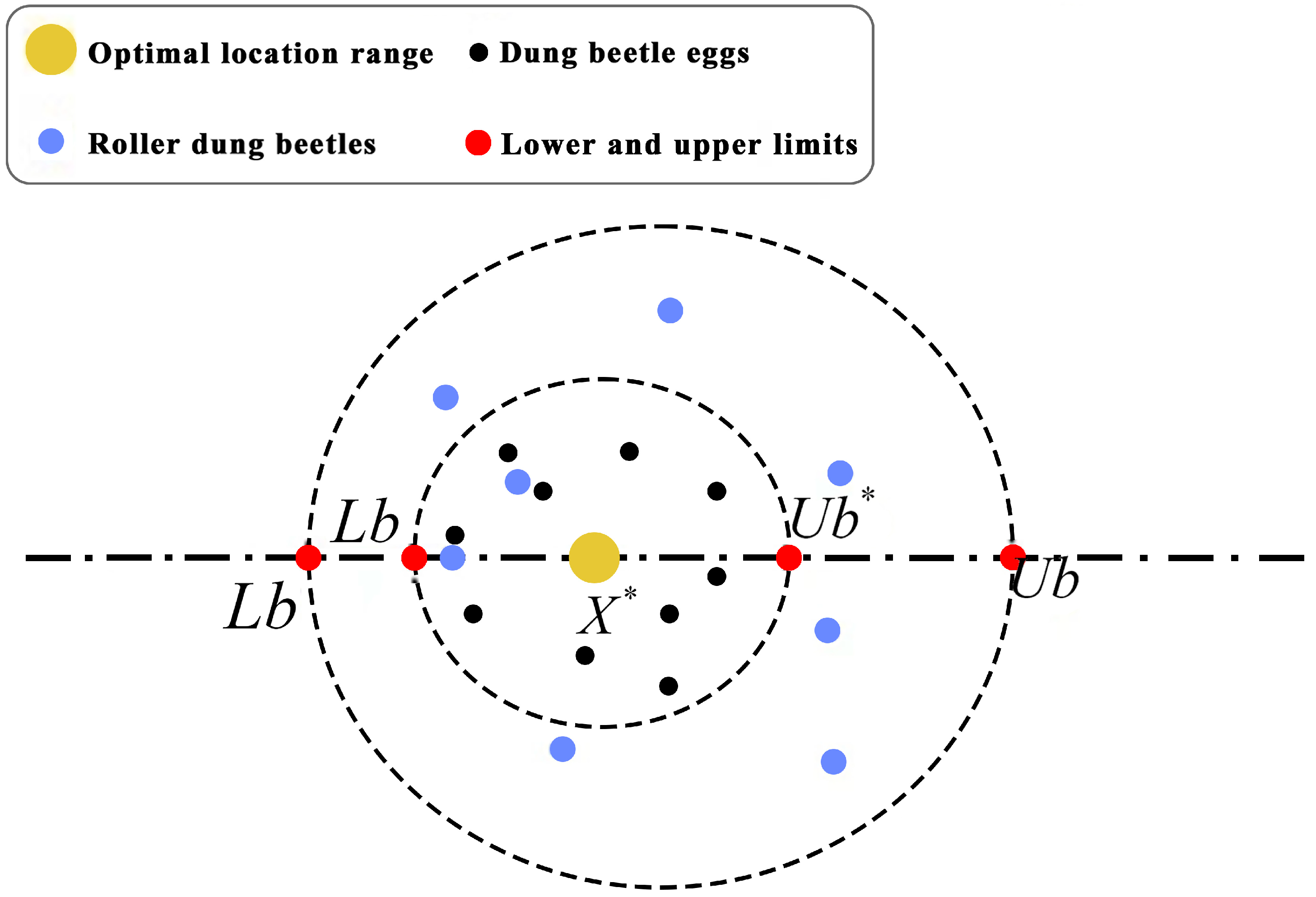
2.1.3. Dung Beetle Reproduction

To provide a safe environment for their offspring, selecting the right oviposition site is crucial for dung beetles. Inspired by the aforementioned discussion, a boundary selection strategy is proposed to simulate the region where female dung beetles lay their eggs [35]. It is defined as follows:

$$L{h}^{\ast }=\max \left(X^{\ast }\ast \left.\left(1-\left.R\right)\right.,Lh\right)\right.$$

(4)

$$U{h}^{\ast }=\min \left(X^{\ast }\ast \left.\left(1-\left.R\right)\right.,Uh\right)\right.$$

(5)

where X* represents the current local best position; Lh* and Uh* denote the upper and lower bounds of the oviposition area, respectively; R = 1 − t/T_max, where T_max represents the maximum iteration count; Lh and Uh are the upper and lower bounds of the search space, respectively.

As shown in Figure 3, it is worth noting that each dung ball contains an egg of a dung beetle. Additionally, the red dots represent the boundaries’ upper and lower limits. In the DBO algorithm, it is assumed that each female dung beetle lays only one egg in each iteration. Due to the dynamic changes in the boundary range during the iteration, this helps prevent the algorithm from getting trapped in local optima, primarily determined by the inertia weight value R. Thus, the position of the egg balls is also dynamic during the iteration process and is defined by the following equation [36]:

$$Y_i(t+1)=X^{\ast }+b_1\left(Y_i(t)-\left.L{h}^{\ast }\right)\right.+b_2\left(Y_i(t)-\left.U{h}^{\ast }\right)\right.$$

(6)

where Y_i(t) represents the position information of the i-th egg ball in the t-th iteration, X* denotes the current local best position, Lh* and Uh* represent the upper and lower bounds of the oviposition area, respectively. $\left(Y_i(t)-\left.L{h}^{\ast }\right)\right.$, $\left(Y_i(t)-\left.U{h}^{\ast }\right)\right.$ denotes the difference between the current position of the egg ball and the upper and lower limits of the oviposition area, b₁ is a random number following a normal distribution, b₂ is a random vector within the range of (0, 1), and D represents the dimension of the optimization problem.

2.1.4. Minor Dung Beetle

Some adult dung beetles burrow into the ground in search of food, and these types of beetles are referred to as minor dung beetles. To simulate the foraging process of minor dung beetles, it is necessary to determine the optimal foraging area [37]. The simulation equation for this area is defined as follows:

$$Lm=\max \left(X^h\ast \left.\left(1-\left.R\right)\right.,Lh\right)\right.$$

(7)

$$Um=\min \left(X^h\ast \left.\left(1-\left.R\right)\right.,Uh\right)\right.$$

(8)

where X^h represents the global best position; Lm and Um are the lower and upper bounds of the optimal foraging area, respectively; Lh and Uh are the lower and upper bounds of the search space. Therefore, the position update for the minor dung beetles is as follows [38]:

$$X_i(t+1)=X_i(t)+C_1\ast \left(X_i(t)-L\mathrm{m}\right)+C_2\left(X_i(t)-U\mathrm{m}\right)$$

(9)

where X_i(t) represents the position of the i-th dung beetle in the t-th iteration; $X_i(t)-L\mathrm{m}$ and $X_i(t)-U\mathrm{m}$ denote the differences between the current dung beetle position and the upper and lower bounds of the optimal foraging area, respectively. C₁ is a randomly generated number following a normal distribution, and C₂ is a random vector within the range of (0, 1).

2.1.5. Thieving Dung Beetle

The position information of the thief is updated as follows during the iteration process, considering that some dung beetles, referred to as thieves, steal dung balls from other beetles. Based on Equation (9), it can be observed that X^h represents the optimal food source. Assuming that the area surrounding X^h represents the prime location for competitive food, the position update for the thief is given by [39]:

$$X_i(t+1)=X^{\mathrm{h}}+W\ast g\ast \left|X_i(t)-X^{\ast }\right|+\left|X_i(t)-X^h\right|$$

(10)

where X_i(t) represents the position information of the i-th thief in the t-th iteration, X^h represents the global best position, X* represents the current local best position, |X_i(t) − X*| and |X_i(t) − X^h| represent the absolute differences between the current position and the local best and global best positions, respectively. g is a randomly generated vector of size 1 × D following a normal distribution, and W is a constant.

Although the DBO algorithm possesses strong optimization capabilities and fast convergence speed, it suffers from the imbalance between global exploration and local exploitation abilities, making it prone to getting stuck in local optima and exhibiting weak global exploration capabilities. To enhance the search performance of DBO, this study proposes four strategies to strengthen DBO.

2.2. Multi-Strategy and Improved Dung Beetle Optimization (MSIDBO) Algorithm

2.2.1. Random Backward Learning Strategy

In swarm intelligence algorithms, the choice of initialization strategy determines the distribution of the initial population in the solution space. In the standard dung beetle algorithm, the population is initialized using a random generation method. Although this approach is simple and easy to implement, randomly generated solutions have certain limitations, as they may fail to cover some potentially good points, thereby slowing down the algorithm’s performance.

To address this issue, this paper adopts a strategy called random reversal learning for population initialization. The random reversal learning strategy [40] generates the reverse position for each individual and evaluates both the original and reverse individuals. The superior individuals are retained for the next generation, enhancing population diversity and avoiding getting trapped in local optima. The specific formula is as follows:

$$X_i^o=Lh+Uh-X_i^t$$

(11)

where $X_i^t$ represents the i-th individual in the population, $X_i^o$ is the corresponding reverse solution to $X_i^t$, and Lh and Uh are the upper and lower limits of individuals in the search space.

To further enhance population diversity and overcome the limitation that the reverse solutions generated by the basic reversal learning strategy may not be better than the current solutions, this paper proposes an improved random reversal learning strategy. By using random reversal learning to generate a reversed population, the search space of the population is expanded, providing more opportunities to discover potential optimal individuals and avoiding the problem of easily getting trapped in local optima during the algorithm’s evolution. The random reversal learning strategy enriches population diversity and effectively improves the exploration capability of the DBO algorithm, which is weaker than its exploitation capability and prone to premature convergence or local stagnation [41]. The specific formula is as follows:

$$X_i^{ro}=Lb+Ub-rand\ast X_i$$

(12)

where $X_i^{ro}$ represents the reverse individual generated by the random reversal learning strategy, and Lb and Ub represent the upper and lower limits of the individual’s position, respectively. $rand\ast X_i$ denotes the random reverse solution, and $X_i$ denotes the reverse solution. rand represents a random number between 0 and 1.

For each individual in the DBO algorithm, the random reversal learning strategy is first applied. This involves simultaneously searching the current solution and its dynamically reversed solution. The better solution is then selected as the initial solution, followed by using other methods for position updates. It is important to note that, to reduce computational cost, during each iteration, each individual is evaluated [42]. If $rand<\frac{t}{T_{\max }}$ (where t represents the iteration count and T_max represents the maximum iteration count), the random reversal learning strategy is executed. Otherwise, the subsequent position update method is directly executed to guide the evolution towards the optimal individual’s position, enhancing the algorithm’s exploration capability and breaking free from the local optima dilemma, leading to improved convergence speed.

2.2.2. Fitness-Distance Balancing (FDB) Strategy

To address the trade-off between diversity and convergence in the population of the DBO algorithm, this paper proposes a fitness-distance balance (FDB) strategy [43]. The FDB strategy is based on the work by Kahraman et al., which relies on both fitness and distance for selection. The objective of this method is to identify one or more candidate solutions that contribute the most to the algorithm’s search process. The key difference of FDB from other selection methods is that the selection process is [44] performed based on the candidates’ scores, not just their fitness values. The score calculation takes into account both the candidates’ fitness function values and their distances to the optimal solution. This ensures that the candidate solution with the highest score is selected to effectively guide the population search. In the stealing process of the DBO algorithm, the thief’s position is influenced by the global best solution, which enables the thief to produce optimal solutions. However, once the optimal individual gets trapped in local optima, the efficiency of the algorithm’s solution process significantly decreases. The FDB algorithm possesses the capability of sensitive searching [45], providing effective diversity, and establishing a strong balance between exploitation and exploration. It can be applied to constrained/unconstrained, unimodal/multimodal/hybrid/combined problem types, and various dimensions. Therefore, this paper incorporates the FDB strategy into the stealing position update equation, where the implementation of the FDB selection method eliminates the local optima problem in the dung beetle algorithm. The specific formula is as follows:

$$X_i(t+1)=X^{FDB}+{\beta }_3\times g\times (\left|X_i(t)-X^{\ast }\right|+\left|X_i(t)-X^{FDB}\right|)$$

(13)

where $X_i(t+1)$ represents the position information of the i-th thief in the (t + 1)-th iteration, $X^{FDB}$ is the candidate solution of the i-th thief selected by the FDB strategy in the t-th iteration, $\left|X_i(t)-X^{\ast }\right|$ represents the absolute difference between the position of the i-th dung beetle in the t-th iteration and its current local best position, $\left|X_i(t)-X^{FDB}\right|$ represents the absolute difference between the position of the i-th dung beetle in the t-th iteration and its candidate position selected through FDB, β is a weighting coefficient, and g is a Gaussian random vector of size 1 × D.

2.2.3. Spiral Foraging Strategy

Figure 4 shows the search models of DBO and MSIDBO algorithm. The original DBO algorithm is prone to getting trapped in local optima, resulting in premature convergence. During the optimization process of DBO, the population gradually converges towards the leader. This search tends to densely explore the vicinity of the current optimal position by following a straight line in each iteration, aiming to improve accuracy and exhibiting strong exploratory capability, as shown in Figure 4a. However, during the approach towards the optimal individual, the exploration of the nearby search space is lost, leading to a reduction in population diversity and an increased likelihood of getting stuck in local optima. If the current optimal position happens to be local optima, it can cause the algorithm to stagnate. To address this issue, this paper introduces a logarithmic spiral search model [46], as depicted in Figure 4b.

From the figure, it can be observed that in each generation, individuals gradually approach their updated positions in a spiral pattern [47], which increases the exploration of the surrounding space and maintains population diversity. This enhances the algorithm’s exploratory capability [48]. Based on this analysis, the dung beetle foraging update formula is adjusted as follows:

$$\beta =e^{bl}\cdot \cos (2\pi b)$$

(14)

$$l=2(1-\frac{t}{t_{\max }})-1$$

(15)

$$X_{\mathrm{i}}(t+1)=X^{\ast }+\beta \times (X_i(t)-L{H}^{\ast })+\beta \times (X_i(t)-U{H}^{\ast })$$

(16)

where b is a constant that determines the shape of the spiral, with a value of 1. β follows a logarithmic function base e, and l is a parameter that linearly decreases from 1 to −1. $X_i(t+1)$ represents the position information of the i-th dung beetle in the (t + 1)-th iteration, $X^{\ast }$ represents the local best position, $(X_i(t)-L{H}^{\ast })$ and $(X_i(t)-U{H}^{\ast })$ represent the difference between the position of the i-th dung beetle in the t-th iteration and the upper and lower limits of the oviposition region.

2.2.4. Optimal Per-Dimension Gaussian Mutation Strategy

To avoid premature convergence, enhance its global search capability, and further improve the performance of multi-objective optimization problems, this paper adopts the Optimal Individual-wise Gaussian Mutation (GM) strategy [49].

Gaussian mutation (GM) is an optimization strategy that applies random numbers following a normal distribution to act on the original position vector in order to generate new positions. It initializes particles adjacent to the target particle with a certain probability, and most of the mutation operators are distributed around the original position, which effectively performs local neighborhood search. This type of mutation not only improves the optimization accuracy of the algorithm but also helps the algorithm escape from local optima. Additionally, the Gaussian mutation randomly initializes particles that exceed the range, with a few operators moving away from the current position. This increases particle utilization and enhances population diversity, facilitating better exploration of potential regions and improving search speed, thereby accelerating the convergence trend of the optimization algorithm [50]. The Gaussian probability density function is defined as follows:

$$f(x)=\frac{1}{\sqrt{2\pi }\sigma }\exp (-\frac{{(x-\mu )}^2}{2{\sigma }^2})$$

(17)

where $\mu$ represents the mean or expected value of the distribution, and $\sigma$ represents the standard deviation. Specifically, in the standard Gaussian probability density function, $\mu$ and $\sigma$ are set to 0 and 1, respectively [51].

To enhance the algorithm’s ability to escape from local optima, at the end of each iteration, the optimal individual obtained is subjected to an Optimal Individual-wise Gaussian Mutation strategy, and a greedy strategy is used to preserve better individuals. In this phase, a Gaussian mutation or Cauchy strategy is applied to each dimension of the optimal individual individually. The specific formula is as follows:

$$X_{new}^b(j)=X^b(j)+(randn\times (X^{rand1}(j)-x^b(j))+randn\times (X^{rand2}(j)-X^b(j)))/2$$

(18)

$$X^b(j)=\left\{\begin{array}{l}{X}_{new}^b(j),if f(X_{new}^b)<f(X^b)\hfill \\ X^b(j),if f(X_{new}^b)\ge f(X^b)\hfill \end{array}\right.$$

(19)

where $X_{new}^b(j)$ represents the j-th dimension of the current optimal individual, $X^b(j)$ represents the j-th dimension of the optimal individual after each iteration, and $X^{rand1}$ and $X^{rand2}$ are randomly selected from the dung beetle population. By using two random individuals ($X^b$) and the current individual ($X_{new}^b$), a new individual is formed and compared with the original individual, overcoming the issues of the DBO algorithm’s susceptibility to local optima and low accuracy.

2.3. The Proposed Algorithm Flowchart

This study proposes a MSIDBO algorithm to overcome the limitations of the traditional DBO algorithm and effectively solve global optimization problems. The MSIDBO algorithm addresses imbalances between global exploration and local exploitation capabilities by introducing a random reverse learning strategy, enhancing population diversity, and mitigating early convergence or local stagnation issues. Additionally, a fitness-distance balancing strategy is incorporated to optimize the trade-off between diversity and convergence within the population. To further improve precision and exploratory capabilities while avoiding local optima, the algorithm utilizes a spiral foraging strategy. Moreover, the MSIDBO algorithm combines the Optimal Dimension-Wise Gaussian Mutation strategy to minimize premature convergence, enhance global search ability, and increase population diversity, thereby accelerating convergence. Figure 5 shows the flow chart of the proposed algorithm. The program flow and steps can be summarized as follows:

Step 1:

Set the percentage of producers (P_percent) in the population.

Step 2:

Calculate the population size of producers (pNum) based on P_percent and the total population size (pop).

Step 3:

Initialize lower bounds (Lb) and upper bounds (Ub) for each dimension.

Step 4:

Initialize the population (x) by randomly selecting grid positions within the bounds.

Step 5:

Evaluate fitness (fit) for each solution in the population.

Step 6:

Set personal best fitness values (pFit) and positions (pX) as the initial fitness values and positions.

Step 7:

Set the current global best fitness value (fMin) and position (bestX) as the minimum fitness value and corresponding position from pFit and pX, respectively.

Step 8:

Start updating the solutions for M iterations: (a) Update a subset of fireflies based on random values and conditions. (b) Apply bounds to the updated solutions. (c) Evaluate fitness for the updated solutions. (d) Determine the current best fitness value (fMMin) and position (bestXX). (e) Update another subset of solutions using Spiral Foraging and FDB Strategy. (f) Apply bounds to the updated solutions. (g) Evaluate fitness for the updated solutions. (h) Update the individual’s best fitness value and global best fitness value if necessary. (i) Random reverse learning and Gaussian mutation to the best solution. (j) Store the best fitness value in the Convergence_curve array.

Step 9:

Termination condition: If the maximum number of iterations (M) is reached, go to step 10. Otherwise, go back to step 8.

Step 10:

Return the global best fitness value (fMin), corresponding position (bestX), and Convergence_curve array.

Figure 5. The proposed algorithm flowchart.

Figure 5. The proposed algorithm flowchart.

3. Simulation Experiment Analysis

3.1. Experiment Environment Simulation

To ensure the rigor and fairness of the experiments, the simulation experiments were conducted using the following hardware and software configurations:

Hardware Environment:

Processor: AMD Ryzen 5 4600 U Radeon [email protected] GHz

Memory: 16 GB DDR4 RAM

Graphics Card: NVIDIA GeForce

Software Environment:

Simulation: MATLAB R2022a

Operating System: Windows 11 (64-bit)

(Note: The configurations of both hardware and software were used for all simulations in this article).

3.2. Experimental Design

To ensure the fairness of the experiments, the parameters were uniformly set as follows: number of runs = 100, maximum iterations = 300, and search agents = 30. A series of numerical experiments were conducted on MSIDBO to validate its effectiveness. Statistical analysis and convergence analysis were performed on 19 test functions. A comparison was made between six algorithms commonly used in recent years: Genetic Algorithms (GA), Grey Wolf Optimization (GWO), Moth-Flame Optimization (MFO), Particle Swarm Optimization (PSO), Whale Optimization Algorithm (WOA) and DBO, and the proposed MSIDBO.

GA is a search method that is also referred to as an evolutionary algorithm that draws inspiration from Darwinian evolution. It simulates the natural and biological evolution process to achieve optimization. The GA algorithm is commonly used for function optimization, data mining, production scheduling, and combination optimization, among other applications. GWO algorithm is a swarm intelligence optimization algorithm that emulates the cooperative behavior of grey wolves to achieve optimization. The GWO algorithm offers advantages such as simplicity, easy implementation, and fast convergence, making it suitable for solving complex optimization problems. MFO is inspired by the movement behavior of moths and the phenomenon of moth flames going extinct. MFOA searches for the optimal solution by simulating moth movement behavior and adjusting parameters based on extinction. PSO is a swarm intelligence algorithm that mimics the social behavior of bird flocks. It optimizes problems by iterating through a population of particles, with each particle representing a potential solution. PSO adjusts particle velocity and position to find the overall best solution. WOA is a nature-inspired algorithm that resembles the search behavior of whales. It leverages social interactions and search patterns to discover global optimal solutions for complex optimization problems. WOA finds application in engineering, data science, operations research, and other fields. DBO is a novel swarm intelligence algorithm that draws inspiration from the ball rolling, dancing, foraging, stealing, and reproduction behaviors of dung beetles. This algorithm incorporates diversified location update strategies to effectively solve complex search and optimization problems.

The superiority of MSIDBO was evaluated by comparing the worst value, best value, average value, and standard deviation (STD) across the 19 benchmark functions. These methods were chosen because they have diverse performance characteristics in exploration and exploitation.

Table 1. Parameter variable settings.

Algorithm	Parameter Variables
MSIDBO	Deviation coefficient K = 0.1, random number b = 0.3, c = 0.5
DBO	Deviation coefficient K = 0.1, random number b = 0.3, c = 0.5
GA	Maximum possible mutation probability $P_{\max }=0.9$, Minimum possible mutation probability $P_{\min }=0.01$
GWO	Convergence factor a linearly decreasing from 2 to 0 during iterations
MFO	Path coefficient $\mathrm{t}\in \left[\mathrm{r},1\right]$, Variable r linearly decreases from −1 to −2
PSO	Learning factor C1 = C2 = 2, Initial inertia weight $W_{\max }=0.9$, Inertia weight at maximum evolution iteration $W_{\min }=0.6$
WOA	Random number for position iteration update $\mathrm{a}\in \left[-1,1\right]$

summarizes the parameter settings for each corresponding algorithm. It is important to note that the values for these parameters were set based on recommendations from their respective reference papers.

3.3. Benchmark Test Functions

To evaluate the performance of the MSIDBO algorithm, a set of 19 benchmark test functions (as shown in

Table 2. Benchmark test functions.

Functions	Dim	Domain	Global Opt
$f_1(x)={\displaystyle \sum _{i=1}^D{x}_i^2}$	50	$\left[-100,100\right]$	0
$f_2(x)={\displaystyle \sum _{i=1}^D\left|x_i\right|}+{\displaystyle \prod _{i=1}^D\left|x_i\right|}$	50	$\left[-100,100\right]$	0
$f_3(x)={{\displaystyle \sum _{i=1}^D\left(\left.{\displaystyle \sum _{j=1}^D{x}_j}\right)\right.}}^2$	50	$\left[-100,100\right]$	0
$f_4(x)=Max\left\{\left.\left|x_i\right|,1\le i\le D\right\}\right.$	50	$\left[-100,100\right]$	0
$f_5(x)={\displaystyle \sum _{i=1}^D\left[100{(x_{i+1}-x_i^2)}^2+{(x_i-1)}^2\right]}$	50	$\left[-30,30\right]$	0
$f_6(x)={\displaystyle \sum _{i=1}^D{\left(\left|x_i+0.5\right|\right)}^2}$	50	$\left[-100,100\right]$	0
$f_7(x)={\displaystyle \sum _{i=1}^{D}i{x}_i^4+random\left[0,1\right]}$	50	$\left[-1.28,1.28\right]$	0
$f_8(x)={\displaystyle \sum _{i=1}^D-x_i\sin (\sqrt{\left|x_i\right|})}$	50	$\left[-500,500\right]$	$-419.98\times Dim$
$f_9(x)={\displaystyle \sum _{i=1}^D\left[x_i^2-10\cos (2\pi x_i)+10\right]}$	50	$\left[-5.12,5.12\right]$	0
$\begin{array}{l}{f}_{10}(x)=-20\exp \left(\left.u\left(x\right)-\exp \left(v(x\left.)\right)+20+e\right.\right)\right.\\ \left\{\begin{array}{c}u(x)=-0.2\sqrt{\frac{1}{d}{\displaystyle \sum _{i=1}^D{x}_i^2}}\\ v(x)=\frac{1}{d}{\displaystyle \sum _{i=1}^D\cos (2\pi x_i)}\end{array}\right.\end{array}$	50	$\left[-32,32\right]$	0
$f_{11}(x)=\frac{1}{4000}{\displaystyle \sum _{i=1}^D{x}_i^2}-{\displaystyle \prod _{i=1}^D\cos \left(\frac{x_i}{\sqrt{i}}\right)+1}$	50	$\left[-600,600\right]$	0
$\begin{array}{l}{f}_{12}(x)=\frac{\pi }{D}\left(v(x)+w(x)+g(x)\right)\\ \left\{\begin{array}{c}v(x)={\displaystyle \sum _{i=1}^D{\left(y_i-1\right)}^2\left[1+10{\sin }^2(\pi y_{i+1})\right]}\\ w(x)=10\sin (\pi y_i)+{\left(y_D-1\right)}^2\\ g(x)={\displaystyle \sum _{i=1}^{D}u(x_i,10,100,4)}\end{array}\right.\end{array}$	50	$\left[-50,50\right]$	0
$\begin{array}{l}{f}_{13}(x)=0.1\left(v(x)+w(x)+g(x)\right)\\ \left\{\begin{array}{c}v(x)={\displaystyle \sum _{i=1}^D{\left(x_i-1\right)}^2\left[1+{\sin }^2(3\pi x_i+1)\right]}\\ w(x)={\sin }^2(3\pi x_i)+{\left(x_D-1\right)}^2\left[1+{\sin }^2(2\pi x_D)\right]\\ g(x)={\displaystyle \sum _{i=1}^{D}u(x_i,5,100,4)}\end{array}\right.\end{array}$	50	$\left[-50,50\right]$	0
$f_{14}(x)={\left(\left.\frac{1}{500}+{\displaystyle \sum _{i=1}^{25}\frac{1}{j+{\displaystyle \sum _{i=1}^2{\left(x_i-a_{ij}\right)}^6}}}\right)\right.}^{-1}$	2	$\left[-65,65\right]$	1
$f_{15}(x)={{\displaystyle \sum _{i=1}^{11}\left[a_i-\frac{x_1(b_i^2+b_i{x}_2)}{b_i^2+b_i{x}_3+x_4}\right]}}^2$	4	$\left[-5,5\right]$	0.0003
$f_{16}(x)=-{\displaystyle \sum _{i=1}^4{c}_i\exp \left(-{\displaystyle \sum _{i=1}^6{a}_{ij}{\left(x_i-p_{ij}\right)}^2}\right)}$	6	$\left[-0,1\right]$	−3.32
$f_{17}(x)=-{{\displaystyle \sum _{i=1}^5\left[\left(X-a_i\right){\left(X-a_i\right)}^T+c_i\right]}}^{-1}$	4	$\left[0,10\right]$	−10.1532
$f_{18}(x)=-{{\displaystyle \sum _{i=1}^7\left[\left(X-a_i\right){\left(X-a_i\right)}^T+c_i\right]}}^{-1}$	4	$\left[0,10\right]$	−10.4028
$f_{19}(x)=-{{\displaystyle \sum _{i=1}^{10}\left[\left(X-a_i\right){\left(X-a_i\right)}^T+c_i\right]}}^{-1}$	4	$\left[0,10\right]$	−10.5363

) were selected for testing. Table 1 summarizes the parameter settings for each corresponding algorithm. It is important to note that the values for these parameters were set based on recommendations from their respective reference papers. Among these functions, f₁ to f₇ are high-dimensional unimodal functions with only one global optimum, which can be used to assess the algorithm’s local exploration capability. Functions f₈ to f₁₃ are high-dimensional multimodal functions, while functions f₁₄ to f₁₉ are fixed-dimension multimodal benchmark functions that have multiple local optima. These functions are suitable for testing the algorithm’s performance in escaping local optima.

3.4. Comparative Analysis with Other Swarm Intelligence Algorithms

The proposed MSIDBO algorithm was independently run 100 times on 19 benchmark functions, along with other population-based intelligent algorithms such as GA, GWO, MFO, PSO, WOA, and DBO. The objective was to evaluate the performance and stability of the proposed algorithm compared to the others in terms of worst value, best value, average value, and standard deviation for dimensions of 30, 60, and 100. The experimental results for different algorithms and dimensions are presented in

Table 3. Experimental results (dim = 30).

Function Name	Metric	GA	GWO	MFO	PSO	WOA	DBO	MSIDBO
f1	Worst	4689.19	2.97 × 10−14	13,302.44	13.17405	341.625	4.1 × 10−53	0
	Best	1.32 × 104	2.70 × 10−16	5.04 × 101	2.86 × 10	3.2 × 10−50	9.8 × 10−91	0
	Average	2.84 × 104	4.70 × 10−15	2.02 × 103	7.00 × 10	8.6 × 10−41	1.37 × 10−54	0
	STD	8.7 × 103	6.37 × 10−15	3.98 × 103	2.56 × 10	1.8 × 10−39	548 × 10−54	0
f2	Worst	83.8083	4.244 × 10−9	78.51766	13.82699	3.6 × 10−28	2.2 × 10−26	3.06 × 10−18
	Best	45.97583	4.34 × 10−10	5.04619	5.64996	2.4 × 10−34	5.2 × 10−47	4.6 × 10−22
	Average	63.22056	1.50 × 10−9	35.05702	9.05261	1.8 × 10−29	7.2 × 10−28	1.1 × 10−184
	STD	9.13277	9.03 × 10−10	19.02526	1.96955	6.7 × 10−29	3.9 × 10−27	0
f3	Worst	96,369.82	0.51767	50,566.01	694.71	1003.13	1.4 × 10−7	0
	Best	2.77 × 104	7.08 × 10−4	8.55 × 103	1.82 × 102	3.1 × 104	7.1 × 10−76	0
	Average	5.48 × 104	6.09 × 10−2	2.55 × 104	3.79 × 102	6.4 × 104	4.5 × 10−9	0
	STD	1.65 × 104	1.12 × 10−1	1.06 × 104	1.20 × 102	1.7 × 104	2.5 × 10−8	0
f4	Worst	86.705	0.0036	83.66176	3.2067	89.26	9.7 × 10−26	1.6 × 10−176
	Best	55.594	0.00017	51.50126	1.7538	2.75654	3.4 × 10−45	7.1 × 10−218
	Average	73.431	0.00096	69.80423	2.4212	53.32	3.2 × 10−27	5.8 × 10−178
	STD	7.702	0.00077	7.991	0.3375	27.27	1.8 × 10−26	0
f5	Worst	1.33 × 108	28.80314	800,769	7165.925	28.81	28.066	26.0072
	Best	885,829	26.10587	7674.538	869.1188	27.67	25.916	24.8950
	Average	453,698	27.40764	4,007,169	2655.264	28.42	26.444	25.4896
	STD	295,623	0.795043	17,096	1453.069	0.34	0.4412	0.2755
f6	Worst	46,613.69	1.8684	15,289.42	14.1803	1.7597	0.36367	2.09 × 10−5
	Best	1.19 × 104	2.05 × 10−1	5.50 × 101	2.99 × 10	2.8 × 10−1	1.8 × 10−3	2.46 × 10−7
	Average	2.76 × 104	1.01 × 10	2.29 × 103	6.95 × 10	8.7 × 10−1	5.8 × 10−2	2.70 × 10−6
	STD	8.63 × 103	4.06 × 10−1	4.45 × 103	2.63 × 10	3.6 × 10−1	9.9 × 10−2	4.14 × 10−6
f7	Worst	54.34306	0.009334	24.65711	94.56221	0.0271	0.0079	0.00059
	Best	5.20 × 10	1.07 × 10−3	1.71 × 10−1	8.86 × 10	2.4 × 10−4	1.8 × 10−4	8.89 × 10−6
	Average	21.60095	0.003818	3.049197	37.29864	0.0060	0.0021	0.00016
	STD	12.37277	0.001928	5.733577	21.47601	0.0067	0.0019	0.00014
f8	Worst	−1290.93	−3474.61	−6702.6	−2963.57	−7243.31	−6060.32	−2 × 1010
	Best	−3387.99	−7725.31	−10,229.3	−7818.69	−12,565.2	−11,415.9	−3 × 1012
	Average	−2160.87	−5955.99	−8484.38	−5438.12	−9912.5	−7973.58	−3 × 1011
	STD	523.1186	922.7797	890.5712	1403.101	1721.52	1310.62	7.1 × 1011
f9	Worst	386.6249	24.65843	247.4207	274.3637	16.6179	34.5862	0
	Best	185.2967	5.32 × 10−9	87.51504	146.6758	0	0	0
	Average	2.91 × 102	7.61 × 10	1.67 × 102	2.12 × 102	5.9 × 10−1	1.3 × 10	0
	STD	4.50 × 101	5.54 × 10	3.78 × 101	2.98 × 101	4.3 × 10	5.1 × 10	0
f10	Worst	426.8172	0.041462	126.051	0.611543	0.1969	0.0227	0
	Best	120.6772	2.88 × 10−15	1.436757	0.188632	0	0	0
	Average	254.698	0.006692	19.0622	0.367474	0.0089	0.0008	0
	STD	77.16924	0.011735	36.4966	0.104	0.0401	0.0043	0
f11	Worst	1.61 × 108	0.241454	419,191	0.909969	0.4626	0.0362	0.00347
	Best	2.76 × 106	1.71 × 10−2	1.18 × 101	4.75 × 10−2	1.1 × 10−2	5.2 × 10−5	5.66 × 10−9
	Average	4.82 × 107	6.39 × 10−2	1.71 × 106	2.41 × 10−1	5.9 × 10−2	3.1 × 10−3	1.16 × 10−4
	STD	4.09 × 107	4.87 × 10−2	8.66 × 106	1.78 × 10−1	8.4 × 10−2	6.9 × 10−3	6.33 × 10−4
f12	Worst	1.64 × 108	0.249422	440,232	0.852634	0.442	0.033	0.0035
	Best	2.75 × 106	1.68 × 10−2	1.21 × 101	4.92 × 10−2	1.1 × 10−2	5.3 × 10−5	5.69 × 10−9
	Average	4.83 × 107	6.45 × 10−2	1.78 × 106	2.35 × 10−1	5.8 × 10−2	2.9 × 10−3	1.16 × 10−4
	STD	4.11 × 107	4.88 × 10−2	8.27 × 106	1.89 × 10−1	8.5 × 10−2	6.9 × 10−3	6.33 × 10−4
f13	Worst	449,511	1.4077	13,866	2.65717	1.498	2.0922	8.37 × 10−6
	Best	1.65 × 107	2.86 × 10−1	9.67 × 101	6.42 × 10−1	2.8 × 10−1	6.2 × 10−2	8.58 × 10−8
	Average	1.47 × 108	8.10 × 10−1	5.20 × 106	1.45 × 10	7.9 × 10−1	1.0 × 10	1.06 × 10−6
	STD	1.06 × 108	2.75 × 10−1	2.73 × 107	4.95 × 10−1	3.1 × 10−1	5.6 × 10−1	1.72 × 10−6
f14	Worst	5.192171	12.66872	9.50493	9.1099	10.975	8.0995	2.967
	Best	0.998	0.998	0.998	0.998	0.998	0.998	0.998
	Average	1.452797	4.8815	2.41707	3.177	3.3345	1.639	1.0791
	STD	0.992756	4.1625	2.14684	2.4604	3.278	1.604	0.3832
f15	Worst	0.059781	0.021665	0.012176	0.00242	0.0041	0.00187	0.00159
	Best	0.00104	0.000312	0.000604	0.000598	0.00032	0.00031	0.00031
	Average	0.014654	0.004761	0.001708	0.000943	0.00083	0.00082	0.0007
	STD	0.013943	0.008261	0.002676	0.000353	0.00074	0.00042	0.00032
f16	Worst	−0.5501	−2.9809	−3.0249	−3.2028	−2.4351	−2.78316	−3.2031
	Best	−2.8874	−3.322	−3.322	−3.322	−3.3215	−3.322	−3.322
	Average	−1.5422	−3.2555	−3.2295	−3.2680	−3.2046	−3.2249	−3.2703
	STD	0.5363	0.0840	0.0654	0.0591	0.1424	0.1085	0.0589
f17	Worst	−0.318	−2.543	−2.631	−2.6305	−1.786	−2.631	−9.706
	Best	−3.126	−10.153	−10.15	−10.1532	−10.2	−10.15	−10.15
	Average	−0.808	−9.040	−6.64	−6.876	−7.68	−7.09	−10.14
	STD	0.485	2.351	3.321	3.23	2.78	2.633	0.067
f18	Worst	−0.411	−4.153	−1.989	−2.3467	−1.708	−2.023	−10.15
	Best	−3.312	−10.402	−10.40	−10.403	−10.40	−10.40	−10.40
	Average	−0.953	−10.217	−7.509	−8.519	−7.045	−8.074	−10.39
	STD	0.492	0.945	3.426	2.978	3.081	2.867	0.03
f19	Worst	−0.594	−2.4372	−2.023	−2.371	−1.62	−2.078	−10.47
	Best	−3.84	−10.54	−10.54	−10.54	−10.53	−10.54	−10.54
	Average	−1.183	−10.191	−7.76	−9.116	−6.597	−8.39	−10.53
	STD	0.4949	1.476	3.54	2.7542	3.276	3.0028	0.01

,

Table 4. Experimental results (dim = 60).

Function Name	Metric	GA	GWO	MFO	PSO	WOA	DBO	MSIDBO
f1	Worst	47,060.83	3.22 × 10−14	15,141.26	13.24628	170.8127	2.78 × 10−53	0
	Best	1.3 × 104	2.52 × 10−16	5.03 × 101	2.87 × 10	6.10 × 10−50	4.91 × 10−91	0
	Average	2.83 × 104	4.89 × 10−15	2.06 × 103	6.91 × 10	1.67 × 10−40	8.65 × 10−55	0
	STD	8.64 × 103	6.85 × 10−15	4.33 × 103	2.53 × 10	9.06 × 10−40	5.08 × 10−54	0
f2	Worst	83.83187	4.25 × 10−9	78.7468	13.9419	5.98 × 10−28	1.094 × 10−26	1.5 × 10−183
	Best	45.73391	4.14 × 10−10	3.849611	5.4771	3.67 × 10−34	2.65 × 10−47	1.46 × 10−217
	Average	63.181247	105 × 10−9	35.11558	9.0236	2.36 × 10−29	3.65 × 10−28	5.11 × 10−185
	STD	9.264722	9.11 × 10−10	19.5689	2.0265	1.11 × 10−28	2.00 × 10−27	0
f3	Worst	97,172.37	0.7521	49,847.9	695.7483	99,905.81	5.7118	0
	Best	2.78 × 104	7.60 × 10−4	8.79 × 103	1.81 × 102	3.14 × 104	3.51 × 10−76	0
	Average	5.51 × 104	6.88 × 10−2	2.52 × 104	3.80 × 102	6.63 × 104	1.90 × 10−1	0
	STD	1.68 × 104	1.44 × 10−4	1.05 × 104	1.20 × 102	1.67 × 104	1.04 × 10	0
f4	Worst	86.884	0.00366	83.62059	3.198605	89.00863	1.917 × 10−24	8.75 × 10−177
	Best	56.1521	0.000168	51.08274	1.7975417	3.145723	4.07 × 10−45	8.69 × 10−26
	Average	73.542202	0.000969	69.6489	0.42622	53.91484	6.40 × 10−26	2.92 × 10−178
	STD	7.696102	0.000786	7.97995	0.332727	27.16403	3.50 × 10−25	0
f5	Worst	1.23 × 108	28.79245	59,238,621	6627.839	28.80585	27.77071	25.9643
	Best	8,811,374	26.09719	7164.07	848.7921	27.66348	25.89962	24.84403
	Average	45,135,450	27.42661	2,806,309	2627.183	28.40701	26.42594	25.47919
	STD	27,999,197	0.79301	12,767,934	1374.001	0.341337	0.400149	0.272682
f6	Worst	46,879.233	1.888057	14,017.877	13.5477	1.62581	0.3568693	1.95 × 10−5
	Best	1.22 × 104	2.10 × 10−1	5.28 × 101	3.04 × 10	2.78 × 10−1	1.70 × 10−3	2.32 × 10−7
	Average	2.77 × 104	9.97 × 10−1	2.31 × 103	6.90 × 10	8.54 × 10−1	5.82 × 10−2	2.70 × 10−6
	STD	8.71 × 103	4.11 × 10−1	4.22 × 103	2.58 × 10	3.41 × 10−1	9.07 × 10−2	4.11 × 10−6
f7	Worst	55.52498	0.009321	26.93012	90.47312	0.002868	0.007282	0.000599
	Best	4.88 × 10	1.12 × 10−3	1.72 × 10−1	8177 × 10	1.92 × 10−4	1.93 × 10−4	9.01 × 10−6
	Average	21.79246	0.003875	3.316123	36.30217	0.00605	0.00206	0.000157
	STD	12.66769	0.001962	6.287797	20.09501	0.006784	0.001723	0.000141
f8	Worst	−1267.73	−3594.26	−6697.17	−2895.65	−7041.94	−6147.06	−2.5 × 1010
	Best	−3409.11	−7652.27	−1010.9	−7839.41	−12,546.6	−11,252.6	−4 × 1012
	Average	−2173.52	−5955.47	−8504.9	−5384.74	−9829.7	−7927.88	−3.6 × 1011
	STD	521.8694	909.7507	878.0597	1418.273	1703.079	287.079	8.1 × 1011
f9	Worst	384.2572	24.70109	246.4823	27.9647	25.67536	30.33065	0
	Best	191.528	4.79 × 10−9	90.29257	146.4949	0	0	0
	Average	2.92 × 102	7.78 × 10	1.66 × 102	2.11 × 102	9.34 × 10−1	1.27 × 10	0
	STD	4.38 × 101	5.92 × 10	3.67 × 101	3.04 × 101	4.76 × 10	5.77 × 10	0
f10	Worst	431.1977	0.039783	137.0223	0.622614	0.228926	0.26325	0
	Best	117.9765	2.95 × 10−15	1.45628	0.181875	0	0	0
	Average	253.767	0.006536	20.4144	0.366436	0.01058	0.001148	0
	STD	77.74329	0.011321	38.43099	0.106027	0.043394	0.004656	0
f11	Worst	1.72 × 108	0.234841	43626794	0.891138	0.334394	0.049533	0.003463
	Best	2.95 × 106	1.80 × 10−2	1.21 × 101	4.83 × 10−2	1024 × 10−2	4.92 × 10−5	6.04 × 10−9
	Average	4.90 × 107	6.39 × 10−2	1.90 × 106	2.38 × 10−1	5.50 × 10−2	3.62 × 10−3	1.15 × 10−4
	STD	4.24 × 107	4.60 × 10−2	8088 × 106	1.85 × 10−1	6.43 × 10−2	1.02 × 10−2	6.32 × 10−4
f12	Worst	1.68 × 108	0.248472	47774328	0.907832	0.337022	0.047568	0.003463
	Best	2.93 × 106	1.80 × 10−2	1.21 × 101	4.81 × 10−2	1.24 × 10−2	5.01 × 10−5	6.00 × 10−9
	Average	4.92 × 107	6.41 × 10−2	1.90 × 106	2.38 × 10−1	5.52 × 10−2	3.62 × 10−3	1.15 × 10−4
	STD	4.27 × 107	4.59 × 10−2	8.88 × 106	1.86 × 10−1	6.42 × 10−2	1.02 × 10−2	6.32 × 10−4
f13	Worst	452,965.6	1.39155	158,787.8	2.67353	1.506665	2.068567	7.067 × 10−6
	Best	1.92 × 107	3.06 × 10−1	1.08 × 102	6068 × 10−1	2.75 × 10−1	8.56 × 10−2	8.21 × 10−8
	Average	1.48 × 108	8.18 × 10−1	5.86 × 106	1.44 × 10	7.82 × 10−1	1.03 × 10	1.12 × 10−6
	STD	1.08 × 108	2.66 × 10−1	3.00 × 107	4.93 × 10−1	3.12 × 10−1	5.41 × 10−1	1.61 × 10−6
f14	Worst	5.600183	12.68501	9.321312	9.360967	11.02894	7.962617	2.618797
	Best	0.9983	0.9981	0.9982	0.998	0.9981	0.9984	0.9982
	Average	1.470307	4.881533	2.420437	3.150983	3.430722	1.662825	1.07296
	STD	1.05 × 10	4.162533	2.13 × 10	2.51 × 10	3.36 × 10	1.61 × 10	3.30 × 10−1
f15	Worst	0.059899	0.021655	0.014185	0.001907	0.004183	0.001909	0.001563
	Best	0.001008	0.000314	0.000605	0.000618	0.000317	0.00308	0.000309
	Average	0.014315	0.004719	0.001788	0.000934	0.000818	0.000827	0.000704
	STD	0.014104	0.008098	0.002943	0.000256	0.000806	0.000431	0.000324
f16	Worst	−0.54294	−2.94784	−3.0336	−3.2028	−2.43004	−2.753082	−3.2031
	Best	−2.8889	−3.322	−3.322	−3.322	−3.3215	−3.322	−3.322
	Average	−1.54377	−3.25589	−3.2285	−3.26701	−3.20363	−3.2237	−3.26929
	STD	0.533095	0.084835	0.06568	0.0592	0.14395	0.110705	0.05909
f17	Worst	−0.319	−2.541	−2.6305	−2.6305	−1849	−2.631	−9.855
	Best	−3.211	−10.15	−10.1532	−10.1532	−10,152	−10.15	−10.15
	Average	−0.815	−8.98	−6.617	−6.8967	−7.7006	−7.013	−10.14
	STD	0.4949	2.398	3.31986	3.2151	2.67675	2.6187	0.35
f18	Worst	−0.414	−3.703	−2.0203	−2.3476	−1.7156	−2.0833	−10,158
	Best	−3.31293	−10.4025	−10.4029	−10.4029	−10.401	−10.403	−104,029
	Average	−0.96489	−10199	−7.548	−8.48659	−7.065	−81,011	−1039
	STD	0.4967	1.0318	3.42173	3.0054	3.0877	2.8608	0.02935
f19	Worst	−0.5987	−2.531	−1.9923	−2.3513	−1.6329	−2.094	−10.474
	Best	−4.265	−10,536	−10.5364	−10.5364	−10.53	−10.536	−105,364
	Average	−1.17597	−10,179	−7.76749	−9.1143	−6.5757	−8.3602	−105,326
	STD	0.4738	1.542	3.54116	2.7224	3.26742	2.99516	0.00961

and

Table 5. Experimental Results (dim = 100).

Function Name	Metric	GA	GWO	MFO	PSO	WOA	DBO	MSIDBO
f1	Worst	47,399.25	3.291 × 10−14	14,797.58	13.157	102.488	2.9 × 10−53	0
	Best	1.30 × 104	2.47 × 10−16	5.14 × 101	2.87 × 10	5.36 × 10−50	3.09 × 10−91	0
	Average	2.82 × 104	5.03 × 10−15	2.10 × 103	6.89 × 10	1.04 × 10−40	9.77 × 10−55	0
	STD	8.65 × 103	7.05 × 10−15	4.30 × 103	2.53 × 10	5.62 × 10−40	5.27 × 10−54	0
f2	Worst	83.9902	4.291 × 10−9	79.884068	13.81985	5.167 × 10−28	7.2 × 10−27	2.07 × 10−183
	Best	45.6242	4.23 × 10−10	3.7710064	5.510094	3.28 × 10−34	1.60 × 10−47	8.74 × 10−218
	Average	63.19297	1.52 × 10−9	35.409994	9.007968	2.05 × 10−29	2.41 × 10−28	6.90 × 10−185
	STD	9.257723	9.13 × 10−10	19.680174	1.99159	9.57 × 10−29	1.31 × 10−27	0
f3	Worst	97,429.1	0.812516	50,226.56	687.1484	99,321.49	3.427076	0
	Best	2.80 × 104	7.42 × 10−4	8.80 × 103	1.82 × 102	3.09 × 104	2.10 × 10−76	0
	Average	5.53 × 104	7.18 × 10−2	2.50 × 104	3.77 × 102	6.32 × 104	1.14 × 10−1	0
	STD	1.65 × 104	1.65 × 10−1	1.05 × 104	1.20 × 102	1.66 × 104	6.26 × 10−1	0
f4	Worst	86.86557	0.003877968	83.975839	3.210732	89.156423	3.42 × 10−24	5.25 × 10−177
	Best	56.00025	0.000169495	50.586567	1.811183	3.54558	3.36 × 10−45	9.52 × 10−214
	Average	73.53378	0.000979805	69.730078	2.430323	54.242383	1.14 × 10−25	1.75 × 10−178
	STD	7.746593	0.000830081	8.088455	0.3305	27.034469	6.24 × 10−25	0
f5	Worst	1.16 × 108	28.77079	43,416,151	6205.322	28.79904	27.55294	25.93408
	Best	8,545,640	26.07047	6957.318	809.3929	27.66108	25.90102	24.87498
	Average	44,424,260	27.38908	2,055,556	2572.316	28.39524	26.40696	25.48113
	STD	26,219,238	0.772878	8,911,164	1299.916	0.341806	0.356248	0.260821
f6	Worst	47,171.09	1.901686	14,914.64	13.559	1.670371	0.3597	1.988 × 10−5
	Best	1.22 × 104	1.97 × 10−1	5.20 × 101	3.00 × 10	2.81 × 10−1	1.68 × 10−3	2.28 × 10−7
	Average	2.78 × 104	9.84 × 10−1	2.24 × 103	6.90 × 10	8.52 × 10−1	5.81 × 10−2	2.75 × 10−6
	STD	8.66 × 103	4.18 × 10−1	4.35 × 103	2.54 × 10	3.43 × 10−1	9.65 × 10−2	4.09 × 10−6
f7	Worst	54.89628	0.009572	27.59129	91.97557	0.027872	0.007225	0.000602
	Best	4.82 × 10	1.08 × 10−3	1.71 × 10−1	8.31 × 10	1.80 × 10−4	1.90 × 10−4	8.67 × 10−6
	Average	21.77833	0.003853	3.337068	36.4818	0.006005	0.002084	0.000159
	STD	12.55115	0.001977	6.293029	20.54151	0.006716	0.001697	0.000142
f8	Worst	−1249.28	−3471.2	−6735.39	−2904.71	−7103.28	−6111.66	−2.5 × 1010
	Best	−3440.29	−7639.39	−10,154.8	−7969.89	−12,554.5	−11,228.6	−3.6 × 1012
	Average	−2169.19	−5951.5	−8515.51	−5400.25	−9857.02	−7914.14	−3.4 × 1011
	STD	528.4644	921.9968	865.4096	1430.685	1713.684	1297.772	7.19 × 1011
f9	Worst	384.278	28.04614	247.2384	272.0869	26.83625	28.64649	0
	Best	198.9717	2.9 × 10−9	91.00348	148.2142	0	0	0
	Average	2.91 × 102	7.88 × 10	1.67 × 102	2.12 × 102	9.43 × 10−1	1.22 × 10	0
	STD	4.41 × 101	6.54 × 10	3.69 × 101	3.02 × 101	4.94 × 10	5.46 × 10	0
f10	Worst	429.6659	0.038694	135.8756	0.616756	0.225699	0.027315	0
	Best	118.4294	2.97 × 10−15	1.452113	0.183202	0	0	0
	Average	2.53 × 102	6.66 × 10−3	2.09 × 101	3.69 × 10−1	1.10 × 10−2	1.05 × 10−3	0
	STD	7.80 × 101	1.12 × 10−2	3.96 × 101	1.05 × 10−1	4.65 × 10−2	5.17 × 10−3	0
f11	Worst	1.74 × 108	0.242085	54,754,976	0.888256	0.347258	0.043088	0.002078
	Best	2.88 × 106	1.77 × 10−2	1.21 × 101	4.86 × 10−2	1.23 × 10−2	4.79 × 10−5	6.05 × 10−9
	Average	4.89 × 107	6.35 × 10−2	2.27 × 106	2.35 × 10−1	5.59 × 10−2	3.23 × 10−3	6.93 × 10−5
	STD	4.27 × 107	4.71 × 10−2	1.09 × 107	1.85 × 10−1	6.61 × 10−2	8.83 × 10−3	3.79 × 10−4
f12	Worst	174,221.5	0.24208463	54,755.74	0.8883	0.3472581	0.043088	0.0020781
	Best	2.88 × 106	1.77 × 10−2	1.21 × 101	4.86 × 10−2	1.23 × 10−2	4.79 × 10−5	6.05 × 10−9
	Average	4.89 × 107	6.35 × 10−2	2.27 × 106	2.35 × 10−1	5.59 × 10−2	3.23 × 10−3	6.93 × 10−5
	STD	4.27 × 107	4.71 × 10−2	1.09 × 107	1.85 × 10−1	6.61 × 10−2	8.83 × 10−3	3.79 × 10−4
f13	Worst	44,047.2	1.398164	171,203.5	2.708498	1.509419	2.060259	7.515 × 10−6
	Best	1.85 × 107	3.16 × 10−1	1.10 × 102	6.57 × 10−1	2.74 × 10−1	8.01 × 10−2	8.26 × 10−8
	Average	1.47 × 108	8.28 × 10−1	6.62 × 106	1.44 × 10	7.80 × 10−1	1.03 × 10	1.12 × 10−6
	STD	1.05 × 108	2.68 × 10−1	3.30 × 107	4.99 × 10−1	3.11 × 10−1	5.44 × 10−1	1.61 × 10−6
f14	Worst	5.52789	12.71625	9.31413	9.255525	11.32096	7.918539	2.403875
	Best	0.998	0.998	0.998	0.998	0.998	0.998	0.998
	Average	1.465371	4.681182	2.450801	3.130818	3.402065	1.66973	1.063373
	STD	1.044614	4.101196	2.141818	2.452627	3.30675	1.602825	0.28916
f15	Worst	0.062858	0.021507	0.013096	0.001702	0.004747	0.001903	0.001509
	Best	0.001024	0.000315	0.000614	0.000618	0.000316	0.000308	0.000308
	Average	0.014875	0.004617	0.001705	0.000926	0.000859	0.000828	0.0007
	STD	0.014875	0.00801	0.002691	0.000216	0.000922	0.000431	0.000324
f16	Worst	−0.5533	−2.962267	−3.00948	−3.202858	−2.470033	−2.748	−3.2031
	Best	−2.896	−3.322	−3.322	−3.322	−3.321454	−3.322	−3.322
	Average	−1.544	−3.256654	−3.228337	−3.267211	−3.20243	−3.223	−3.268901
	STD	0.5293	0.08392682	0.06586	0.05924	0.14353	0.1103	0.059099
f17	Worst	−0.317	−2.557448	−2.6305	−2.6305	−1.904	−2.631	−9.8866
	Best	−3.389	−10.1527	−10.153	−10.153	−10.152	−10.15	−10.153
	Average	−0.817	−8.97082	−6.5838	−6.9079	−7.6909	−6.989	−10.142
	STD	0.505	2.39862	3.3139	3.2124	2.7723	2.6069	0.03235
f18	Worst	−0.419	−3.7898	−1.9655	−2.336	−1.724	−2.129	−10.226
	Best	−3.326	−10.4024	−10.403	−10.41	−10.401	−10.41	−10.403
	Average	−0.96	−10.194	−7.5417	−8.449	−7.0764	−8.11	−10.396
	STD	0.4899	1.04452	3.422	3.017	3.088	2.8644	0.0224
f19	Worst	−0.591	−2.5181	−1.9941	−2.34	−1.6243	−2.12	−10.477
	Best	−4.24	−10.5359	−10.536	−10.536	−10.53	−10.54	−10.536
	Average	−1.173	−10.17441	−7.7544	−9.104	−6.559	−8.363	−10.533
	STD	0.4729	1.561447	3.5422	2.7467	3.2594	2.9881	0.00928

. These results provide insights into the superior search performance and stability of the proposed algorithm compared to other population-based intelligent algorithms.

For unimodal functions f₁ and f₃ (Table 3), the theoretical optimum can only be found by the proposed MSIDBO algorithm, with both a mean and standard deviation equal to 0. DBO performs relatively worse, with the smallest negative mean values being closest to 0. In f₂ and f₄, only the standard deviation of the MSIDBO algorithm is 0. Among f₅, f₆, and f₇, MSIDBO finds all optimal solutions, with DBO performing second-best, while GWO, PSO, and MFO exhibit inferior performance. Regarding multimodal functions, in f₉ and f₁₀, only the MSIDBO algorithm is capable of finding the theoretical optimum, with both mean and standard deviation equal to 0. In fixed-dimensional functions f₁₃ to f₁₉, MSIDBO achieves the best values, demonstrating significant and distinctive superiority: the standard deviation of MSIDBO is consistently one or more orders of magnitude better than other algorithms.

According to Table 4, for unimodal functions, it can be observed that only the MSIDBO algorithm can find the theoretical optimum, with both mean and standard deviation equal to 0 in f₁ and f₃. In f₂ and f₄, only the standard deviation of the MSIDBO algorithm is 0, followed by DBO. MSIDBO outperforms other algorithms in terms of various metrics in f₅ to f₇, particularly in f₆. The mean and standard deviation of MSIDBO are several orders of magnitude smaller (negative) compared to other algorithms, which are on the order of −2 or higher. When observing multimodal functions f₈ to f₁₃, the differences among the values of various algorithms are not significant. However, the advantage of MSIDBO still persists, as it consistently achieves optimal search results. It is worth noting that in f₈ to f₁₃, the values obtained by GA are noticeably larger than those of other algorithms, indicating its weaker algorithmic performance compared to others.

In Table 5, for unimodal functions, it can be observed that only the MSIDBO algorithm can find the theoretical optimum, with both mean and standard deviation equal to 0 in f₁ and f₃. In f₂ and f₄, only the standard deviation of the MSIDBO algorithm is 0. Furthermore, in f₅ to f₇, MSIDBO exhibits the smallest standard deviation, indicating greater stability. For fixed-dimensional functions, specifically in f₁₇ to f₁₉, the standard deviation of GWO is significantly larger than that of other algorithms, indicating its poor stability. Among the three dimensions, data for dim = 60 and dim = 100 are similar in nature. In these cases, MSIDBO shows relatively minor fluctuations across different dimensions, demonstrating strong stability. Conversely, the other algorithms exhibit more noticeable fluctuations. GA displays the largest standard deviation and least stability, followed by PSO, GWO, and MFO, all of which experience varying degrees of reduced convergence speed and susceptibility to dimension changes.

Based on the above analysis, it can be observed that MSIDBO exhibits a more significant competitive advantage in solving unimodal, multimodal, and fixed-dimensional functions. To provide a more intuitive comparison of the algorithms’ convergence accuracy and speed, this study plotted the convergence curves of the test functions based on the number of iterations and fitness values (refer to Figure 6, Figure 7 and Figure 8). Figure 9 illustrates the two-dimensional shapes of some test functions used to evaluate the MSIDBO algorithm.

Upon observing Figure 6, Figure 7 and Figure 8, it can be noted that for functions f₁, f₃, f₁₀, f₁₁, f₁₅, and f₁₆, MSIDBO consistently converges to the global optimal solution with a success rate of 100%. The convergence accuracy of MSIDBO is significantly better than the other six algorithms, which fail to find the global optimum. In f₁, f₂, f₃, f₄, and f₈, MSIDBO distributes the population more evenly across the solution space, increasing the number of individuals near the optimal solution. Consequently, the algorithm quickly finds the optimal solution within a few iterations, resulting in nearly linear convergence curves in the figures. Regarding local exploitation capability, MSIDBO outperforms the selected well-known algorithms on the tested functions. In terms of computational time, MSIDBO requires significantly less iterations to find the optimal solution compared to other algorithms: in f₁ to f₈, f₁₀, and f₁₃, MSIDBO quickly identifies the optimal value with 250–300 iterations, performing thorough exploration. In f₉ and f₁₀, the convergence iterations range from 50 to 100, while in f16, it is less than 50, indicating faster convergence and smoother stability. By examining the average convergence curves of high-dimensional multimodal functions (f₈ to f₁₃), it becomes evident that MSIDBO achieves higher optimization accuracy. It demonstrates superior exploration capability in finding the optimal solutions for these multimodal functions. For fixed-dimensional functions (f₁₅ to f₁₉), due to the complexity of the algorithms, the curves for all methods appear similar with minimal differences. However, MSIDBO still exhibits slightly better performance as it converges quickly in the early stages of iteration. The results indicate that in terms of exploration capability, the MSIDBO algorithm consistently outperforms other methods in both convergence speed and accuracy, demonstrating superior global search ability and the capability to escape local optima.

From a different perspective, the figures reveal that compared to other algorithms, MSIDBO achieves satisfactory convergence speed in functions f₁–f₁₃. This can be attributed to the algorithm’s ability to thoroughly explore promising regions in the early iterations. MSIDBO exhibits the fastest optimization process among the 19 benchmark functions, effectively saving optimization time, and converging to the global optimal position as quickly as possible in the later stages. As a result, the chances of MSIDBO getting trapped in local optima are significantly lower than those of other methods, whereas other algorithms tend to become trapped in local optima in the later stages and struggle to escape. Overall, the MSIDBO algorithm consistently demonstrates superior convergence speed and accuracy compared to other methods.

3.5. Effectiveness Analysis of Improvement Strategies

Compared to other well-known algorithms, MSIDBO has shown a certain level of improvement in solution accuracy and more stable average optimization performance. This indicates that the introduced random reversed learning strategy enhances the algorithm’s global exploration capability and generates highly diverse initial dung beetle populations. Additionally, the convergence curve gradually deepens its exploration when the convergence speed slows down, indicating that MSIDBO, with the embedded fitness distance balancing strategy, effectively balances the diversity and convergence within the population, as well as the global exploration and local exploitation abilities. The introduced spiral foraging strategy improves optimization stability, enhances initial population diversity, and strengthens the ability for rapid iterative optimization while avoiding local optima and premature convergence. The incorporation of optimal individual-wise Gaussian mutation strategy significantly enhances the algorithm’s exploitation capability, and its fast convergence curve suggests that the Gaussian mutation strategy effectively avoids getting trapped in local optima and improves the algorithm’s optimization ability.

From the algorithms such as MFO, PSO, and GA mentioned in this article, it can be observed that swarm intelligence algorithms currently encounter several issues including slow convergence speed, easily falling into local optima, low solving accuracy, and limited stability. To address these problems, the MSIDBO algorithm is proposed in this study, incorporating a random reverse learning strategy to enhance population diversity. Additionally, the algorithm adopts a fitness distance balance strategy to effectively address the trade-off between diversity and convergence within the population. Moreover, the integration of a spiral foraging strategy in the algorithm enhances search accuracy and mitigates local optima. By combining the MSIDBO algorithm with the optimal dimensional Gaussian mutation strategy, premature convergence is reduced, global search capabilities are strengthened, and convergence speed is accelerated. The research outcomes hold significant importance in the areas of algorithm development and path planning. The proposal and verification of the MSIDBO algorithm significantly contribute to the existing body of knowledge on swarm intelligence-based optimization techniques and their practical applications. Notably, these findings hold great potential in practical applications such as robotics, autonomous navigation, and search and rescue missions. Efficient path planning plays a critical role in ensuring effective mobility in complex environments. The MSIDBO algorithm’s ability to generate globally optimal paths while considering obstacle avoidance can substantially enhance the performance and reliability of such systems. Furthermore, the research outcomes contribute to the academic understanding of algorithm design and optimization strategies. The integration of various strategies within the MSIDBO algorithm, along with the introduction of the novel spiral foraging technique, offers a fresh perspective on path algorithm enhancements. These findings not only address current challenges with innovative solutions but also represent advancements in the field. Moreover, the research results have the potential to impact and improve existing algorithms. As a response to the limitations and deficiencies discovered in the original DBO algorithm, the MSIDBO provides an improved alternative for path planning. Researchers and practitioners can benefit from these findings by integrating the proposed strategies into their own or leveraging specific aspects of the MSIDBO algorithm to enhance their existing techniques.

In conclusion, regardless of unimodal, multimodal, fixed-dimension, or different dimensional problems, MSIDBO is capable of accurately finding the optimal values. It exhibits adaptive transitions between global exploration and local exploitation, demonstrating excellent performance. By comparison, the MSIDBO algorithm not only achieves higher final convergence accuracy than other algorithms, but also converges faster. Its convergence speed is significantly advantageous, while maintaining high convergence accuracy, allowing for quick search and convergence, and further improvements.

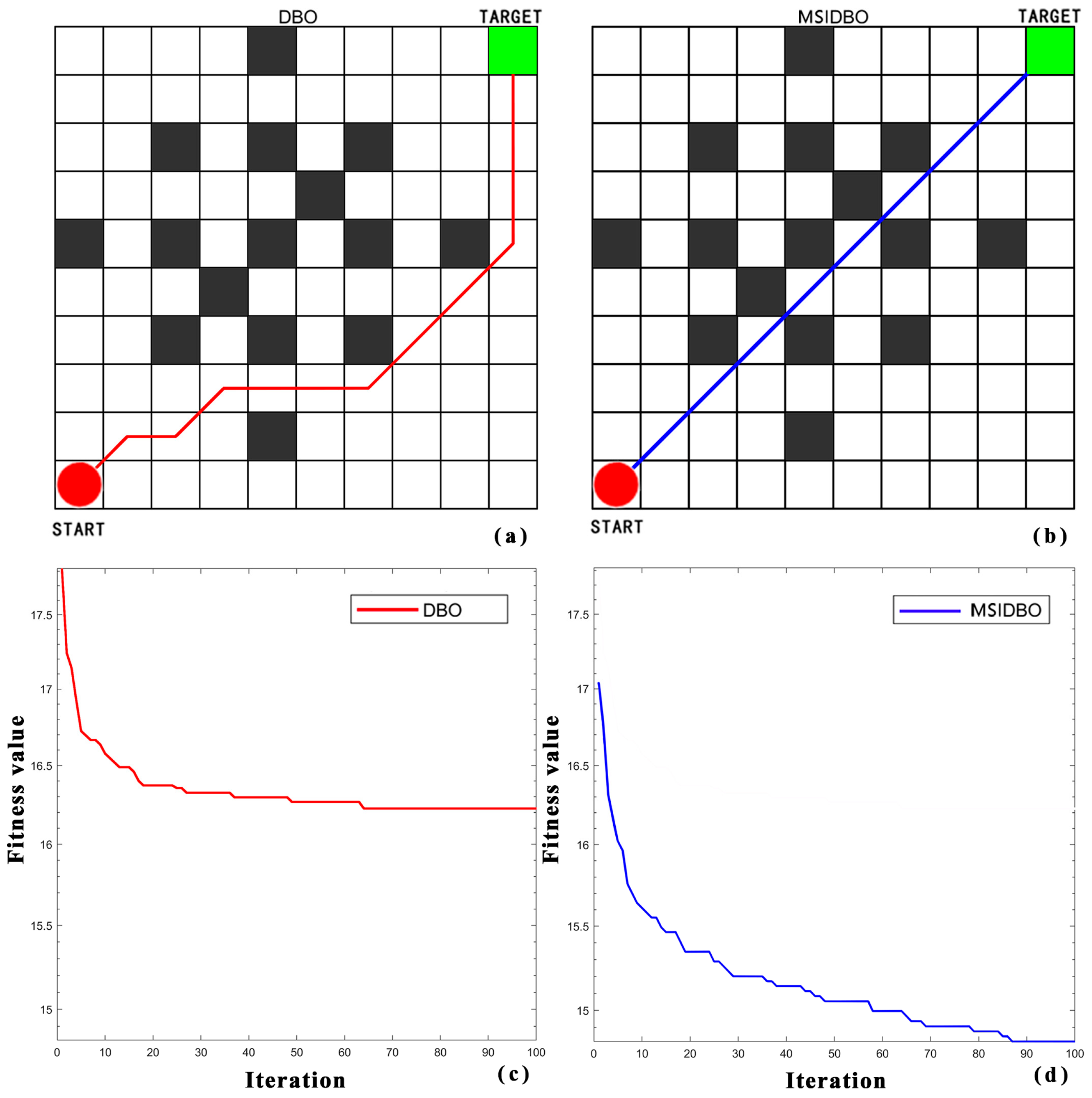
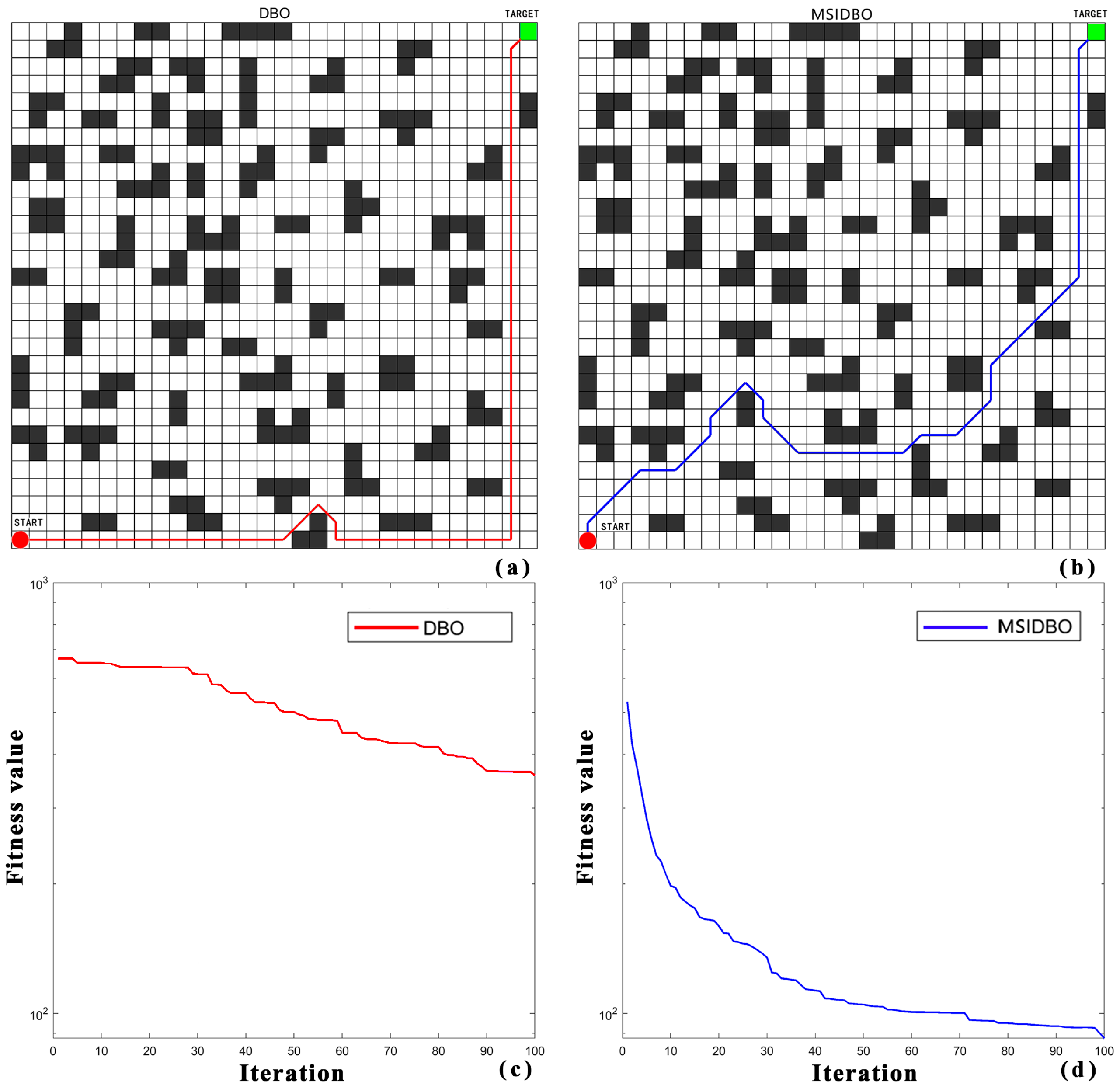
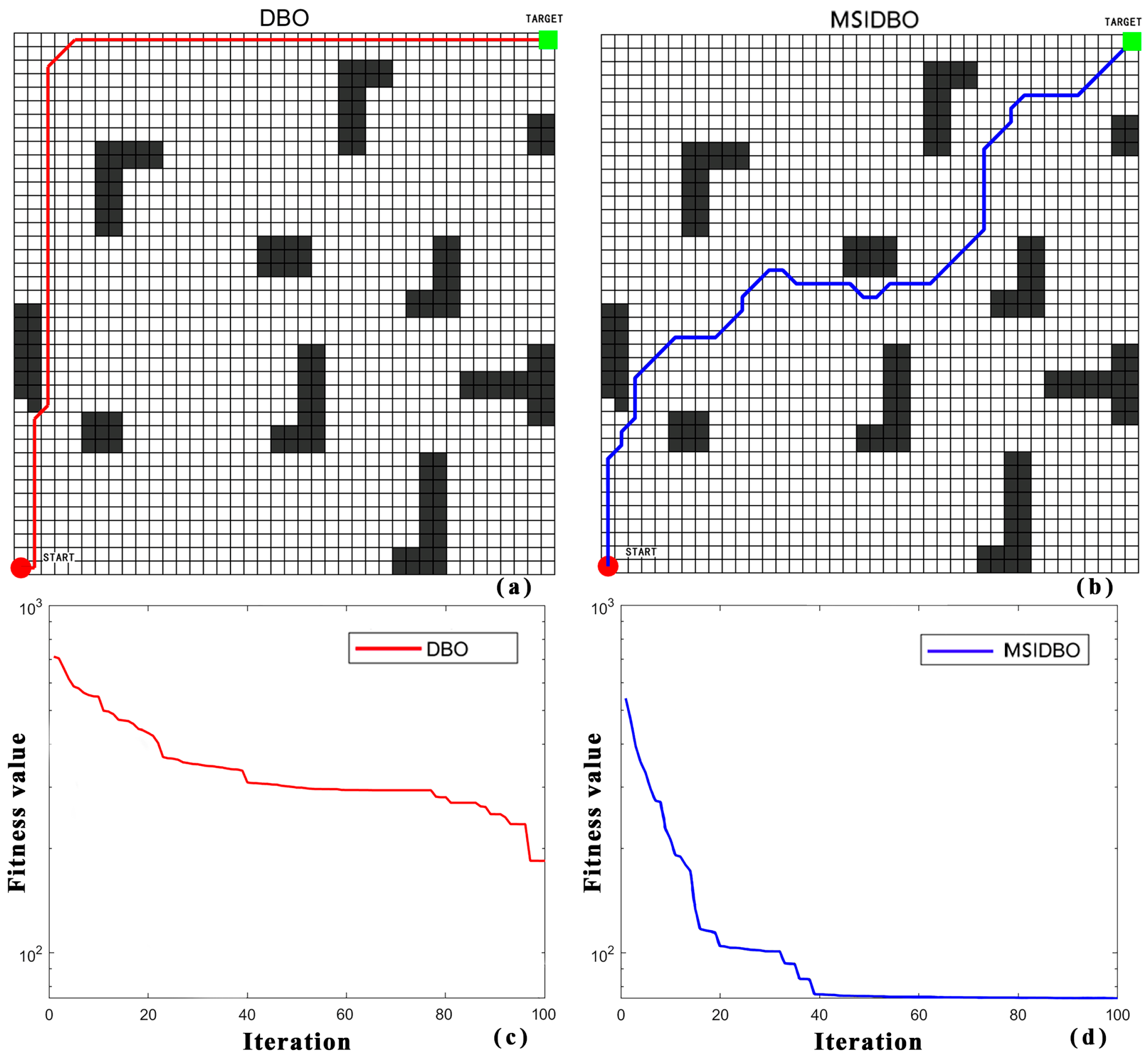
4. Simulation and Validation of Path Planning Experiments

To further validate the capabilities and effectiveness of the MSIDBO algorithm in path planning, this study adopts grid-based modeling to represent a known environment. MATLAB simulation software is utilized to conduct comparative experiments between the MSIDBO and DBO algorithms, exploring their performance on grid maps of varying sizes (10 × 10, 15 × 15, 20 × 20, 30 × 30, and 40 × 40) with a grid distance of 1 m. Different obstacle rates are employed to construct grids with various complexities. In these grid maps, black cells denote obstacles, while white cells indicate areas where the algorithms can navigate. The robot is represented as a point entity equipped with perception capabilities to detect and comprehend obstacles and target points within the grid map.

The evaluation of the generated paths encompasses assessing their completeness in reaching the designated targets, analyzing path lengths for efficiency evaluation, ensuring collision avoidance with obstacles, and quantifying the number of turns and iterations involved in the paths to evaluate the results. The number of turns reflects the complexity of the path planning process, while the number of iterations signifies the level of iterative optimization achieved by the algorithm.

By independently running the standard MSIDBO and DBO algorithms, both initialized with identical population sizes and a maximum iteration count of 100, we compare their performances. The starting and ending points of the paths are located at the bottom left and top right corners of the grid map, respectively. Each algorithm undergoes 50 independent runs, and the average values are computed as the final outcomes. The path trajectories are shown in Figure 10, Figure 11, Figure 12, Figure 13, Figure 14, Figure 15, Figure 16, Figure 17, Figure 18, Figure 19, Figure 20, Figure 21, Figure 22, Figure 23 and Figure 24, while the metric test results are presented in

Table 6. Metrics comparison of the runs.

Map Size	Obstacle Rate	Metric	DBO	MSIDBO	Decrease Percentage (%)
10 × 10	10%	Path Length (m)	14.4853	14.1532	2.29%
		Number of Turns	6	4	33.33%
		Iteration	90	80	11.11%
	15%	Path Length (m)	15.05	12.73	15.41%
		Number of Turns	5	0	100.00%
		Iteration	90	88	2.22%
	20%	Path Length (m)	14.46	13.28	13.54%
		Number of Turns	5	3	40%
		Iteration	92	65	29.35%
15 × 15	10%	Path Length (m)	25.65685	20.38478	20.55%
		Number of Turns	6	4	33.33%
		Iteration	91	78	14.29%
	15%	Path Length (m)	25.31371	20.97056	17.16%
		Number of Turns	15	5	66.67%
		Iteration	63	50	20.63%
	20%	Path Length (m)	22.14214	20.38478	7.94%
		Number of Turns	10	4	60%
		Iteration	90	83	7.78%
20 × 20	10%	Path Length (m)	34.4853	33.3137	3.40%
		Number of Turns	10	7	30.00%
		Iteration	80	70	12.50%
	15%	Path Length (m)	35.64	30.92	13.24%
		Number of Turns	8	13	−6.25%
		Iteration	72	67	6.94%
	20%	Path Length (m)	43.56	30.63	29.68%
		Number of Turns	19	11	42.11%
		Iteration	96	76	20.83%
30 × 30	10%	Path Length (m)	55.64	51.47	7.49%
		Number of Turns	5	17	−70.58%
		Iteration	56	50	10.71%
	15%	Path Length (m)	60.93	52.57	13.72%
		Number of Turns	11	7	36.37%
		Iteration	97	80	17.53%
	20%	Path Length (m)	57.72	54.08	6.31%
		Number of Turns	6	16	−166.67%
		Iteration	110	100	9.09%
40 × 40	10%	Path Length (m)	75.24	68.53	8.92%
		Number of Turns	5	23	−360.00%
		Iteration	93	42	54.84%
	15%	Path Length (m)	188.94	77.74	58.85%
		Number of Turns	46	29	36.96%
		Iteration	90	80	11.11%
	20%	Path Length (m)	76.83	72.73	5.34%
		Number of Turns	4	9	−175.00%
		Iteration	95	91	4.21%

.

In Figure 10, Figure 11, Figure 12, Figure 13, Figure 14, Figure 15, Figure 16, Figure 17, Figure 18, Figure 19, Figure 20, Figure 21, Figure 22, Figure 23 and Figure 24, it can be observed that due to MSIDBO being an optimization of the base algorithm DBO, there are similarities in the path planning. In Figure 11b, the path planned by MSIDBO is a straight line. In Figure 13a,b, Figure 14a,b and Figure 18a,b, it can be seen that the paths generated by MSIDBO are simpler, smoother, and more stable compared to DBO. When the convergence speed slows down, MSIDBO delves deeper into exploration by increasing the diversity of the initial population, enhancing its ability for rapid iterative optimization while avoiding local optima and premature convergence. Therefore, the paths generated by MSIDBO are smoother with fewer turning points, shorter in length, require less search time, effectively avoid obstacles, and achieve ordered visits to all waypoints, finding the optimal solution with less iteration. On the other hand, the paths generated by DBO have more turning points, longer lengths, lack smoothness, and exhibit insufficient local exploration capabilities during subsequent iterations, leading the algorithm to become trapped in local optima.

By observing the convergence curves, it can be seen that under the same maximum iteration count, the convergence curve of the MSIDBO algorithm is smoother and tends to stabilize earlier and faster. Additionally, from the graphs, it is apparent that the DBO path planning contains numerous turning points and transitions, indicating that DBO is prone to getting trapped in local optima and struggles to escape from them. Conversely, the MSIDBO curve in many cases approximates a steep line, with minimal instances of being stuck in local optima. Even if it does get trapped, it quickly escapes and finds the optimal solution. Considering the overall observations in Figure 17, Figure 19, Figure 20, Figure 21 and Figure 22 in complex maps, MSIDBO tends to generate optimal paths near the diagonal of the map. This ensures the generation of relatively optimal paths while significantly improving the speed of path finding. As the map size increases, this effect becomes more pronounced, and MSIDBO performs better on larger-sized maps. On the other hand, the DBO algorithm generates paths on the outer parts of the map where there are fewer obstacles. In such cases, although the number of turns decreases, the path length becomes longer. DBO performs relatively well in small-sized maps with slightly fewer turning points and approaches the optimal solution. However, as the map size increases, the number of turning points increases, leading to multiple instances of getting trapped in local optima and deviating further from the optimal solution.

To compare the two algorithms more clearly and precisely, this study summarizes and compares the path length, number of turns, and iteration count in Table 6 and Figure 25. The table also includes the corresponding reduction rates for path length, number of turns, and iteration count achieved by the MSIDBO algorithm. Figure 25 shows the performance comparisons between DBO and MSIDBO. By comparing the data in Table 6, it can be observed that MSIDBO performs better than DBO in terms of path length, number of turns, and iteration count. It is worth noting that in maps shown in Figure 17, Figure 19, Figure 20, Figure 21, Figure 22 and Figure 23, the number of turns in MSIDBO is greater than that in DBO. However, MSIDBO still outperforms DBO in terms of path length and iteration count. Therefore, the performance of MSIDBO remains superior to DBO. Satisfactorily, in Figure 10, the number of turns in MSIDBO reduced by 100%. In Figure 23, the path length in MSIDBO decreased by 58.85%. In Figure 22, the iteration count decreased by 54.84%. As the map size increases, the advantages of MSIDBO become more pronounced, particularly in optimizing smaller-sized maps, indicating its broader applicability. This clearer observation highlights that MSIDBO provides significant optimization over DBO in all aspects. It successfully avoids the central region with multiple obstacles, resulting in a shorter path length, lower variance in path length, better stability unaffected by map size, and fewer turning points. The algorithm runs smoothly and is more suitable for finding optimal paths in complex obstacle environments.

5. Conclusions

The paper begins by introducing the principles and mathematical model of the DBO algorithm. Addressing the limitations of the original DBO algorithm, such as the imbalance between global exploration and local exploitation capabilities leading to a tendency for local optima and weaker global exploration abilities, the study proposes improvements. The revised strategies are elaborated upon in detail. Subsequently, 19 benchmark test functions are selected for simulation and a thorough comparison between the improved MSIDBO and DBO algorithms is carried out. The experimental results demonstrate that the improved algorithm not only ensures the generation of relatively optimal paths but also significantly improves the speed of pathfinding. This improvement becomes more pronounced with increasing map size. Applying the enhanced algorithm in path planning experiments further confirms that MSIDBO meets practical requirements by generating shorter and smoother paths while exhibiting faster convergence. It shows adaptability in complex environments, making it highly suitable. Additionally, by effectively utilizing the advantages of both global and local planning methods, the proposed algorithm successfully addresses the problem of local obstacle avoidance when a global route has already been planned. This enhances obstacle avoidance performance while guaranteeing globally optimal planned paths, resulting in significant optimization effects. Therefore, in scenarios involving complex maps or emphasizing real-time computation, the MSIDBO algorithm exhibits strong application advantages.

The research findings are highly significant in the fields of algorithm development and path planning. By proposing and demonstrating the effectiveness of the MSIDBO algorithm, the contributes to the existing knowledge on swarm intelligence-based optimization techniques and their applications. One major aspect of the research findings is their potential value in practical applications such as robotics, autonomous navigation, and search and rescue missions. Effective path planning plays a crucial role in ensuring efficient movement in complex and dynamic environments in these applications. The MSIDBO algorithm’s ability to generate globally optimal paths while considering obstacle avoidance can greatly enhance the performance and reliability of such systems. Moreover, the research findings contribute to the academic community by expanding the understanding of algorithm design and optimization strategies. The integration of multiple strategies in the MSIDBO algorithm, along with the introduction of the novel spiral foraging technique, presents new perspectives on how to improve path planning algorithms. This not only provides innovative solutions for current challenges, but also progress in the field. Furthermore, the research findings have the potential to influence and improve existing algorithms. By addressing the limitations and drawbacks of the original DBO algorithm, the MSIDBO algorithm offers an alternative and improved approach to path planning. Other researchers and practitioners can benefit from these findings by incorporating the proposed strategies into their own algorithms or leveraging specific aspects of the MSIDBO algorithm to enhance their existing techniques.

References

1. Jiang, S.; Hong, Z. Unexpected Dynamic Obstacle Monocular Detection in the Driver View. IEEE Intell. Transp. Syst. Mag. 2022, 15, 68–81. [Google Scholar] [CrossRef]
2. Ait Saadi, A.; Soukane, A.; Meraihi, Y.; Benmessaoud Gabis, A.; Mirjalili, S.; Ramdane-Cherif, A. UAV path planning using optimization approaches: A survey. Arch. Comput. Methods Eng. 2022, 29, 4233–4284. [Google Scholar] [CrossRef]
3. Yan, C.; Xiang, X.; Wang, C. Towards real-time path planning through deep reinforcement learning for a UAV in dynamic environments. J. Intell. Robot. Syst. 2020, 98, 297–309. [Google Scholar] [CrossRef]
4. Puente-Castro, A.; Rivero, D.; Pazos, A.; Fernandez-Blanco, E. A review of artificial intelligence applied to path planning in UAV swarms. Neural Comput. Appl. 2022, 34, 153–170. [Google Scholar] [CrossRef]
5. Yao, Q.; Zheng, Z.; Qi, L. Path planning method with improved artificial potential field—A reinforcement learning perspective. IEEE Access 2020, 8, 135513–135523. [Google Scholar] [CrossRef]
6. Kandathil, J.J.; Mathew, R.; Hiremath, S.S. Development and analysis of a novel obstacle avoidance strategy for a multi robot system inspired by the bug-1 algorithm. Simulation 2020, 96, 807–824. [Google Scholar] [CrossRef]
7. Huang, S.K.; Wang, W.J.; Sun, C.H. A Path Planning Strategy for Multi-Robot Moving with Path-Priority Order Based on a Generalized Voronoi Diagram. Appl. Sci. 2021, 11, 9650. [Google Scholar] [CrossRef]
8. Alshammrei, S.; Boubaker, S. Improved Dijkstra Algorithm for Mobile Robot Path Planning and Obstacle Avoidance. Comput. Mater. Contin. 2022, 72, 5939–5954. [Google Scholar] [CrossRef]
9. Ma, X.; Gong, R.; Tan, Y. Path planning of mobile robot based on improved PRM based on cubic spline. Wirel. Commun. Mob. Comput. 2022, 2022, 1632698. [Google Scholar] [CrossRef]
10. Kang, J.G.; Lim, D.W.; Choi, Y.S. Improved RRT-Connect Algorithm Based on Triangular Inequality for Robot Path Planning. Sensors 2021, 21, 333. [Google Scholar] [CrossRef]
11. Wang, J.; Chi, W.; Li, C.; Wang, C.; Meng, M.Q.H. Neural RRT*: Learning-based optimal path planning. IEEE Trans. Autom. Sci. Eng. 2020, 17, 1748–1758. [Google Scholar] [CrossRef]
12. Chi, W.; Ding, Z.; Wang, J.; Chen, G.; Sun, L. A generalized Voronoi diagram-based efficient heuristic path planning method for RRTs in mobile robots. IEEE Trans. Ind. Electron. 2021, 69, 4926–4937. [Google Scholar] [CrossRef]
13. Pehlivanoglu, Y.V.; Pehlivanoglu, P. An enhanced genetic algorithm for path planning of autonomous UAV in target coverage problems. Appl. Soft Comput. 2021, 112, 107796. [Google Scholar] [CrossRef]
14. Patle, B.K.; Pandey, A.; Parhi, D.R.K.; Jagadeesh, A.J.D.T. A review: On path planning strategies for navigation of mobile robot. Def. Technol. 2019, 15, 582–606. [Google Scholar] [CrossRef]
15. Mohanty, P.K.; Dewang, H.S. A smart path planner for wheeled mobile robots using adaptive particle swarm optimization. J. Braz. Soc. Mech. Sci. Eng. 2021, 43, 101. [Google Scholar] [CrossRef]
16. Wu, L.; Huang, X.; Cui, J. Modified adaptive ant colony optimization algorithm and its application for solving path planning of mobile robot. Expert Syst. Appl. 2023, 215, 119410. [Google Scholar] [CrossRef]
17. Ge, H.; Ying, Z.; Chen, Z. Improved A* Algorithm for Path Planning of Spherical Robot Considering Energy Consumption. Sensors 2023, 23, 7115. [Google Scholar] [CrossRef]
18. Zhang, G.; Zhang, E. An improved sparrow search based intelligent navigational algorithm for local path planning of mobile robot. J. Ambient. Intell. Humaniz. Comput. 2023, 14, 14111–14123. [Google Scholar] [CrossRef]
19. Guo, F.; Zhang, H.; Xu, Y.; Xiong, G.; Zeng, C. Isokinetic Rehabilitation Trajectory Planning of an Upper Extremity Exoskeleton Rehabilitation Robot Based on a Multistrategy Improved Whale Optimization Algorithm. Symmetry 2023, 15, 232. [Google Scholar] [CrossRef]
20. Gao, L.; Liu, R.; Wang, F. An Advanced Quantum Optimization Algorithm for Robot Path Planning. J. Circuits Syst. Comput. 2020, 29, 2050122. [Google Scholar] [CrossRef]
21. Hong, K.R.; Park, J.K.; Kim, U.C. Rao-combined artificial bee colony algorithm for minimum dose path planning in complex radioactive environments. Nucl. Eng. Des. 2022, 400, 112043. [Google Scholar] [CrossRef]
22. Li, Y.; Wang, G. Sand cat swarm optimization based on stochastic variation with elite collaboration. IEEE Access 2022, 10, 89989–90003. [Google Scholar] [CrossRef]
23. Jiang, S.; Yao, W.; Wong, M.S.; Hang, M.; Hong, Z.; Kim, E.J. Automatic elevator button localization using a combined detecting and tracking framework for multi-story navigation. IEEE Access 2019, 8, 1118–1134. [Google Scholar] [CrossRef]
24. Dong, L.; Yuan, X.; Yan, B. An Improved Grey Wolf Optimization with Multi-Strategy Ensemble for Robot Path Planning. Sensors 2022, 22, 6843. [Google Scholar] [CrossRef] [PubMed]
25. Li, K.; Hu, Q.; Liu, J. Path Planning of Mobile Robot Based on Improved Multiobjective Genetic Algorithm. Wirel. Commun. Mob. Comput. 2021, 2021, 8881684. [Google Scholar] [CrossRef]
26. Zhu, F.; Li, G.; Tang, H. Dung beetle optimization algorithm based on quantum computing and multi-strategy fusion for solving engineering problems. Expert Syst. Appl. 2023, 236, 121219. [Google Scholar] [CrossRef]
27. Zhang, R.; Zhu, Y. Predicting the Mechanical Properties of Heat-Treated Woods Using Optimization-Algorithm-Based BPNN. Forests 2023, 14, 935. [Google Scholar] [CrossRef]
28. Wang, Z.; Huang, L.; Yang, S. A quasi-oppositional learning of updating quantum state and Q-learning based on the dung beetle algorithm for global optimization. Alex. Eng. J. 2023, 81, 469–488. [Google Scholar] [CrossRef]
29. Shen, Q.; Zhang, D.; Xie, M. Multi-Strategy Enhanced Dung Beetle Optimizer and Its Application in Three-Dimensional UAV Path Planning. Symmetry 2023, 15, 1432. [Google Scholar] [CrossRef]
30. Xue, J.; Shen, B. Dung beetle optimizer: A new meta-heuristic algorithm for global optimization. J. Supercomput. 2023, 79, 7305–7336. [Google Scholar] [CrossRef]
31. Jin, H.; Ji, H.; Yan, F. An Effective Obstacle Avoidance and Motion Planning Design for Underwater Telescopic Arm Robots Based on a Tent Chaotic Dung Beetle Algorithm. Electronics 2023, 12, 4128. [Google Scholar] [CrossRef]
32. Qin, L.; Li, T.; Shi, M. Internal leakage rate prediction and unilateral and bilateral internal leakage identification of ball valves in the gas pipeline based on pressure detection. Eng. Fail. Anal. 2023, 153, 107584. [Google Scholar] [CrossRef]
33. Xiao, Y.; Zhang, H.; Wang, R. Low-Carbon and Energy-Saving Path Optimization Scheduling of Material Distribution in Machining Shop Based on Business Compass Model. Processes 2023, 11, 1960. [Google Scholar] [CrossRef]
34. Wu, C.; Fu, J.; Huang, X.; Xu, X.; Meng, J. Lithium-Ion Battery Health State Prediction Based on VMD and DBO-SVR. Energies 2023, 16, 3993. [Google Scholar] [CrossRef]
35. Zhu, X.; Ni, C.; Chen, G.; Guo, J. Optimization of Tungsten Heavy Alloy Cutting Parameters Based on RSM and Reinforcement Dung Beetle Algorithm. Sensors 2023, 23, 5616. [Google Scholar] [CrossRef] [PubMed]
36. Guo, X.; Qin, X.; Zhang, Q.; Zhang, Y.; Wang, P.; Fan, Z. Speaker Recognition Based on Dung Beetle Optimized CNN. Appl. Sci. 2023, 13, 9787. [Google Scholar] [CrossRef]
37. Zilong, W.; Peng, S. A Multi-Strategy Dung Beetle Optimization Algorithm for Optimizing Constrained Engineering Problems. IEEE Access 2023, 11, 98805–98817. [Google Scholar] [CrossRef]
38. Dong, Y.H.; Yu, Z.C.; Hu, T.Y. Inversion of Rayleigh wave dispersion curve based on improved dung beetle optimizer algorithm. Pet. Geol. Recovery Effic. 2023, 30, 86–97. [Google Scholar]
39. Alamgeer, M.; Alruwais, N.; Alshahrani, H.M. Dung Beetle Optimization with Deep Feature Fusion Model for Lung Cancer Detection and Classification. Cancers 2023, 15, 3982. [Google Scholar] [CrossRef]
40. Mohapatra, S.; Mohapatra, P. Fast random opposition-based learning Golden Jackal Optimization algorithm. Knowl.-Based Syst. 2023, 275, 110679. [Google Scholar] [CrossRef]
41. Ali, M.A.S.; PP, F.R.; Salama Abd Elminaam, D. A Feature Selection Based on Improved Artificial Hummingbird Algorithm Using Random Opposition-Based Learning for Solving Waste Classification Problem. Mathematics 2022, 10, 2675. [Google Scholar] [CrossRef]
42. Balakrishnan, K.; Dhanalakshmi, R.; Mahadeo Khaire, U. Excogitating marine predators algorithm based on random opposition-based learning for feature selection. Concurr. Comput. Pract. Exp. 2022, 34, e6630. [Google Scholar] [CrossRef]
43. Kahraman, H.T.; Aras, S.; Gedikli, E. Fitness-distance balance (FDB): A new selection method for meta-heuristic search algorithms. Knowl.-Based Syst. 2020, 190, 105169. [Google Scholar] [CrossRef]
44. Wang, K.; Tao, S.; Wang, R.L. Fitness-distance balance with functional weights: A new selection method for evolutionary algorithms. IEICE Trans. Inf. Syst. 2021, 104, 1789–1792. [Google Scholar] [CrossRef]
45. Tasci, D.A.; Kahraman, H.T.; Kati, M. Improved Gradient-Based Optimizer with Dynamic Fitness Distance Balance for Global Optimization Problems. Smart Appl. Adv. Mach. Learn. Hum.-Centred Probl. Des. 2023, 1, 247. [Google Scholar]
46. Li, X.; Yang, Q.; Wu, H. Joints Trajectory Planning of Robot Based on Slime Mould Whale Optimization Algorithm. Algorithms 2022, 15, 363. [Google Scholar] [CrossRef]
47. Zhang, X.Y.; Hao, W.K.; Wang, J.S. Manta ray foraging optimization algorithm with mathematical spiral foraging strategies for solving economic load dispatching problems in power systems. Alex. Eng. J. 2023, 70, 613–640. [Google Scholar] [CrossRef]
48. Yang, C.; Yang, H.; Zhu, D. Chaotic sparrow search algorithm with manta ray spiral foraging for engineering optimization. Syst. Sci. Control Eng. 2023, 11, 2249021. [Google Scholar] [CrossRef]
49. Song, S.; Wang, P.; Heidari, A.A. Dimension decided Harris hawks optimization with Gaussian mutation: Balance analysis and diversity patterns. Knowl.-Based Syst. 2021, 215, 106425. [Google Scholar] [CrossRef]
50. Zhang, X.; Xu, Y.; Yu, C. Gaussian mutational chaotic fruit fly-built optimization and feature selection. Expert Syst. Appl. 2020, 141, 112976. [Google Scholar] [CrossRef]
51. Zhou, W.; Wang, P.; Heidari, A.A. Spiral Gaussian mutation sine cosine algorithm: Framework and comprehensive performance optimization. Expert Syst. Appl. 2022, 209, 118372. [Google Scholar] [CrossRef]
Figure 1. Dung beetle trajectory model.
Electronics 12 04462 g001
Figure 2. Tangent function and dancing model of dung beetles. (a) Tangent function in the rolling direction; (b) dancing model of dung beetles.
Electronics 12 04462 g002
Figure 3. Concept model of boundary selection strategy.
Electronics 12 04462 g003
Figure 4. Search models. (a) search model of DBO algorithm; (b) logarithmic spiral search model.
Electronics 12 04462 g004
Figure 6. Convergence processes of different algorithms for a unimodal function. Subfigures (ag) correspond to functions f1f7, respectively.
Electronics 12 04462 g006
Figure 7. Convergence processes of different algorithms for a multimodal function. Subfigures (af) correspond to functions f8f13, respectively.
Electronics 12 04462 g007
Figure 8. Convergence processes of different algorithms for a fixed-dimensional multimodal function. Subfigures (af) correspond to functions f14f19, respectively.
Electronics 12 04462 g008
Figure 9. Plots of the 19 standard benchmark functions. Subfigures (as) represent functions f1f19, respectively. Different colors represent different numerical values, with lighter colors leading to larger values.
Electronics 12 04462 g009
Figure 10. Path planning comparison graph (10 × 10, obstacle rates 10%). Panels (a) and (b) present the outcomes obtained from the DBO and MSIDBO algorithms, respectively, applied to path planning. Panels (c) and (d) provide descriptive fitness value iteration curves corresponding to the DBO and MSIDBO algorithms. Note that Figure 11, Figure 12, Figure 13, Figure 14, Figure 15, Figure 16, Figure 17, Figure 18, Figure 19, Figure 20, Figure 21, Figure 22, Figure 23 and Figure 24 have similar meanings to Figure 10, but with differences in map size, complexity, and obstacle rate.
Electronics 12 04462 g010
Figure 11. Path planning comparison graph (10 × 10, obstacle rates 15%). Panels (a) and (b) present the results of DBO and MSIDBO algorithms for path planning, respectively. Panels (c) and (d) depict the fitness value-iterations curves for DBO and MSIDBO algorithms, respectively.
Electronics 12 04462 g011
Figure 12. Path planning comparison graph (10 × 10, obstacle rates 20%). Panels (a) and (b) present the results of DBO and MSIDBO algorithms for path planning, respectively. Panels (c) and (d) depict the fitness value-iterations curves for DBO and MSIDBO algorithms, respectively.
Electronics 12 04462 g012
Figure 13. Path planning comparison graph (15 × 15, obstacle rates 10%). Panels (a) and (b) present the results of DBO and MSIDBO algorithms for path planning, respectively. Panels (c) and (d) depict the fitness value-iterations curves for DBO and MSIDBO algorithms, respectively.
Electronics 12 04462 g013
Figure 14. Path planning comparison graph (15 × 15, obstacle rates 15%). Panels (a) and (b) present the results of DBO and MSIDBO algorithms for path planning, respectively. Panels (c) and (d) depict the fitness value-iterations curves for DBO and MSIDBO algorithms, respectively.
Electronics 12 04462 g014
Figure 15. Path planning comparison graph (15 × 15, obstacle rates 20%). Panels (a) and (b) present the results of DBO and MSIDBO algorithms for path planning, respectively. Panels (c) and (d) depict the fitness value-iterations curves for DBO and MSIDBO algorithms, respectively.
Electronics 12 04462 g015
Figure 16. Path planning comparison graph (20 × 20, obstacle rates 10%). Panels (a) and (b) present the results of DBO and MSIDBO algorithms for path planning, respectively. Panels (c) and (d) depict the fitness value-iterations curves for DBO and MSIDBO algorithms, respectively.
Electronics 12 04462 g016
Figure 17. Path planning comparison graph (20 × 20, obstacle rates 15%). Panels (a) and (b) present the results of DBO and MSIDBO algorithms for path planning, respectively. Panels (c) and (d) depict the fitness value-iterations curves for DBO and MSIDBO algorithms, respectively.
Electronics 12 04462 g017
Figure 18. Path planning comparison graph (20 × 20, obstacle rates 20%). Panels (a) and (b) present the results of DBO and MSIDBO algorithms for path planning, respectively. Panels (c) and (d) depict the fitness value-iterations curves for DBO and MSIDBO algorithms, respectively.
Electronics 12 04462 g018
Figure 19. Path planning comparison graph (30 × 30, obstacle rates 10%). Panels (a) and (b) present the results of DBO and MSIDBO algorithms for path planning, respectively. Panels (c) and (d) depict the fitness value-iterations curves for DBO and MSIDBO algorithms, respectively.
Electronics 12 04462 g019
Figure 20. Path planning comparison graph (30 × 30, obstacle rates 15%). Panels (a) and (b) present the results of DBO and MSIDBO algorithms for path planning, respectively. Panels (c) and (d) depict the fitness value-iterations curves for DBO and MSIDBO algorithms, respectively.
Electronics 12 04462 g020
Figure 21. Path planning comparison graph (30 × 30, obstacle rates 20%). Panels (a) and (b) present the results of DBO and MSIDBO algorithms for path planning, respectively. Panels (c) and (d) depict the fitness value-iterations curves for DBO and MSIDBO algorithms, respectively.
Electronics 12 04462 g021
Figure 22. Path planning comparison graph (40 × 40, obstacle rates 10%). Panels (a) and (b) present the results of DBO and MSIDBO algorithms for path planning, respectively. Panels (c) and (d) depict the fitness value-iterations curves for DBO and MSIDBO algorithms, respectively.
Electronics 12 04462 g022
Figure 23. Path planning comparison graph (40 × 40, obstacle rates 15%). Panels (a) and (b) present the results of DBO and MSIDBO algorithms for path planning, respectively. Panels (c) and (d) depict the fitness value-iterations curves for DBO and MSIDBO algorithms, respectively.
Electronics 12 04462 g023
Figure 24. Path planning comparison graph (40 × 40, obstacle rates 20%). Panels (a) and (b) present the results of DBO and MSIDBO algorithms for path planning, respectively. Panels (c) and (d) depict the fitness value-iterations curves for DBO and MSIDBO algorithms, respectively.
Electronics 12 04462 g024
Figure 25. Performance comparisons between DBO and MSIDBO. (a) metric values; (b) MSIDBO overperformance ratio.
Electronics 12 04462 g025