Output Feedback Control of Overhead Cranes Based on Disturbance Compensation

Abstract

In practice, various factors such as friction, unmodeled dynamics and uncertain external disturbances often affect overhead cranes. The existing crane control methods often neglect these factors or address these factors by robust techniques. Moreover, most of them do not take input saturation into account and require full-state feedback. In this paper, taking the practical issues of uncertain disturbances, input saturation and output feedback into account, we propose an input-saturated output feedback control strategy for the underactuated two-dimensional (2-D) overhead crane systems with uncertain disturbances. Specifically, we first design a disturbance observer that can accurately estimate the external disturbance. Then, the virtual horizontal location signal is introduced and the new energy storage function is constructed. A novel composite control method for overhead crane systems is proposed based on the developed disturbance observer and the new energy storage function. The stability and convergence analysis are given through Lyapunov techniques and LaSalle’s invariance theorem. In order to verify the performance of the proposed controller, we perform a series of simulation tests and compare the proposed method with some existing control methods.

1. Introduction

In recent years, underactuated mechatronic systems, with more degrees of freedom than control inputs, have been widely used in real-world applications. Such systems include inverted pendulums [1,2], ball and beam systems [3], underactuated aircraft, vessels [4,5,6,7], suspension systems [8,9], etc., and have received extensive attention from the control community; a lot of meaningful research results on this topic have been reported in the literature [10,11,12,13]. Among them, the overhead crane system is also a common underactuated mechatronic system. On the one hand, the merits of the underactuated overhead crane system include a simple mechanical structure, less energy consumption, lower hardware cost, high carrying capacity and more flexible work; hence, they are widely used for cargo transportation in various sites. On the other hand, due to the complex nonlinear characteristics and underactuated features of the overhead cranes, the control problems of the overhead crane system present great challenges. During the transfer process, due to its own inertia and the existence of various external disturbances, there is always an undesired payload swing. This seriously affects the efficiency of the control system, making it difficult to unload cargo. Uncontrolled residual oscillations may even pose a serious safety threat to the people around.

Up to today, more and more scholars have devoted themselves to design effective controllers for overhead cranes to realize satisfactory control. As a result, a large number of control methods have been reported in the literature, which can be roughly classified into open-loop and closed-loop control methods. For the open-loop control methods, the input shaping technique [14,15,16] has been demonstrated to be effective for crane control and is widely used. Additionally, based on the highly coupled kinematics of overhead cranes, trajectory planning methods [17,18,19,20,21] are also proposed for the crane systems. In particular, in [20], a novel off-line minimum-time trajectory planning method is proposed, which simultaneously takes various constraints into account, including the bounded payload swing angle, acceleration, bounded velocity and even jerk for the trolley. However, due to the absence of a feedback mechanism, the open-loop control methods are sensitive to system parameter variations and external disturbances.

The other control method that has been usually designed for the control of the overhead crane systems is the closed-loop control method, which presents robustness to external disturbances and parameter variations because of the system state feedback. In recent years, a large number of closed-loop methods have been proposed to enhance the safety and transport efficiency of overhead crane systems. In particular, based on the passivity property of the overhead crane system, several energy-based controllers [22,23,24] have been proposed to achieve satisfactory control performances. However, these methods require exact model knowledge. In order to achieve adaptability to system parameter uncertainty and external disturbances, some adaptive control methods have been proposed in [25,26,27,28,29]. To deal with uncertain disturbances, the sliding mode control technique has been developed for overhead crane systems in [30,31,32,33]. In particular, in [30], a continuous sliding mode controller is designed to ensure that the state variables remain on the sliding manifold. On this basis, a nonlinear disturbance observer is introduced to compensate for external disturbances. The main advantage of this controller is that it does not sacrifice controller performance and is highly robust to external disturbances. In addition, model predictive control (MPC) [34,35,36,37] has also been applied to crane systems because of its advantages in handling constraints, ability to exploit simple models and robustness to parameter uncertainties. The approach proposed in [36] achieves low energy consumption and a small swing angle at the same time. In addition to the aforementioned methods, numerous intelligent controllers [38,39,40], including fuzzy logic controllers and a neural network, have been applied to solve the control issues of crane systems.

By summarizing the existing methods, we find that many issues are not well considered during the control design. Most existing closed-loop control methods of overhead cranes require full-state feedback. However, in most conditions due to insufficient sensor accuracy and so on, the exact velocity signals are unavailable. Additionally, the existing control methods are designed by assuming that the actuator can provide any bounded control force and the input constraints are not taken into account. The output the actuator can provide is limited; if the input exceeds the allowable range, it will cause the actuator to saturate and destroy the system stability. In addition, the overhead crane system will inevitably be subject to uncertain interference in practical applications. The existing sliding mode control methods usually eliminate these disturbances in a robust way, which means sacrificing the controller’s performance.

With the motivation to address the above three issues associated with the existing methods for the overhead crane system, we suggest a novel nonlinear control method, which simultaneously takes these three practical issues into account. Therefore, the proposed control method here exhibits three remarkable features: output feedback, bounded amplitude and robustness to uncertain external disturbances. Specifically, we first transform the crane dynamics into a form convenient for controller design through a series of auxiliary variables. After that, we design a nonlinear disturbances observer that can estimate unknown external disturbances within a certain time. Next, we suggest a novel control method for the overhead crane system based on a disturbance observer, which relies on a virtual horizontal location signal derived from its dynamic model. We then rigorously prove that the state variables converge to the equilibrium point. Finally, to examine the performance of the method designed in this paper, simulation tests are carried out and a comparison study is provided.

In summary, the main contributions of this work are summarized as follows.

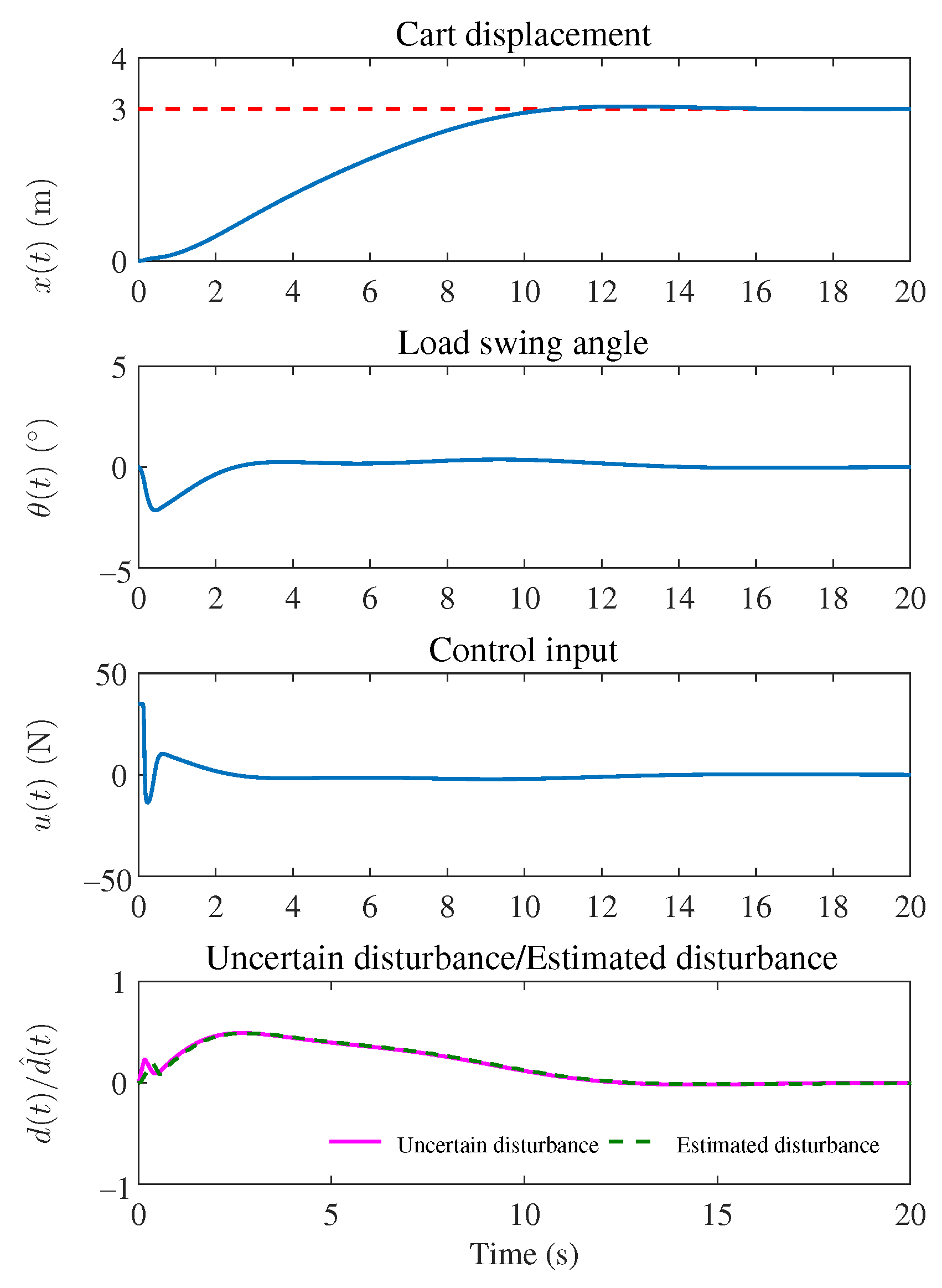
• Uncertain external disturbances are estimated and compensated through a feedforward control way, which hence enhances the robustness of the overhead crane system.
• The practical problem of actuators providing only limited force is taken into consideration. The amplitude of the proposed control method can be set on the basis of the practical actuators.
• The designed controller uses only output feedback, that is, the proposed approach does not require the velocity sensors in real applications, which can reduce hardware costs.

The remainder of this article is organized as follows. In Section 2, we give a brief introduction to crane dynamics. Section 3 presents a nonlinear disturbance observer and a nonlinear control strategy and analyzes their stability and convergence. In Section 4, the simulation results are provided to verify the regulation performance and strong robustness of the proposed method. Finally, the main contributions of this paper are summarized in Section 5.

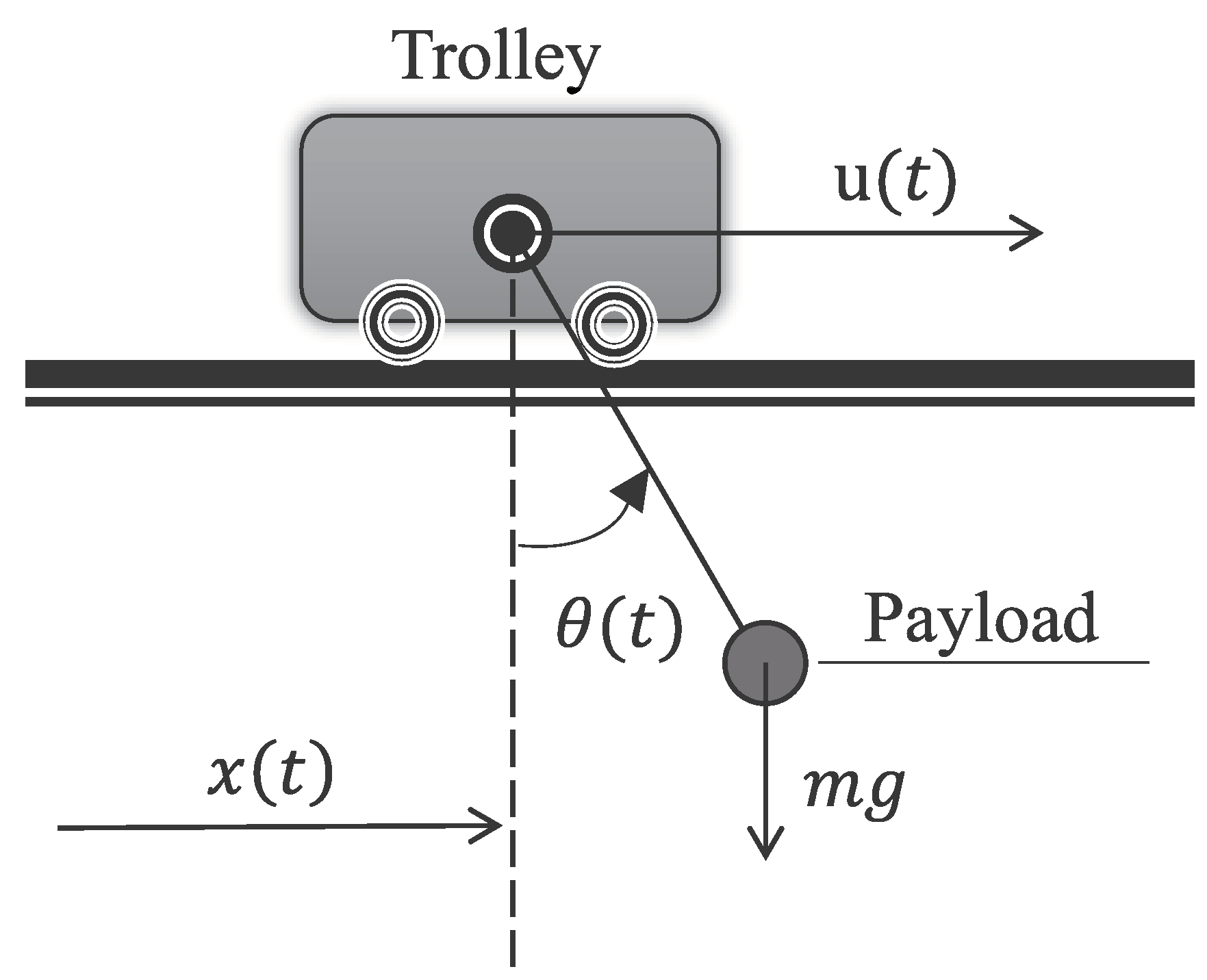
2. Dynamic Model of the Overhead Crane System

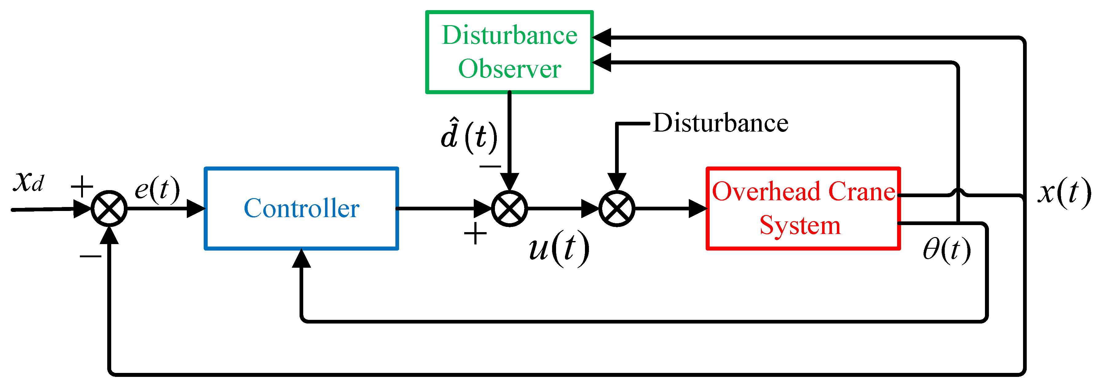
To investigate the control of the two-dimensional (2-D) overhead crane system (shown in Figure 1), the dynamic model of the 2-D overhead crane system is represented by [24,26,30,41]

$$\begin{array}{cc}\hfill & (M+m)\ddot{x}+ml\ddot{\theta }cos\theta -ml{\dot{\theta }}^{2}sin\theta =u+d\hfill \end{array}$$

(1)

$$\begin{array}{cc}\hfill & m{l}^2\ddot{\theta }+mlcos\theta \ddot{x}+mglsin\theta =0\hfill \end{array}$$

(2)

where variable $\theta \left(t\right)$ represents the payload swing angle, and variable $x\left(t\right)$ denotes the trolley displacement. m is the payload mass, and M represents the trolley mass. l stands for the length of the rope, and g is the gravitational constant.

The variable $u\left(t\right)$ represents the control input; considering the practical working conditions for overhead cranes, the force provided by the actuator is bounded, so the control input $u\left(t\right)$ should have the upper bound as follows:

$$\begin{array}{cc}\hfill & \left|u\left(t\right)\right|\le u_m\hfill \end{array}$$

(3)

where $u_m\in {\mathbb{R}}^{+}$ is an a priori known, positive bounding constant and depends on the actuator selected.

In the meantime, the lumped disturbance term $d\left(t\right)$ consists of friction, unmodeled dynamics, uncertain external disturbances and so forth. Considering the actual conditions, we assume that the lumped term $d\left(t\right)$ has the upper bound

$$\begin{array}{cc}\hfill & \left|d\left(t\right)\right|\le \overline{d},\left|\dot{d}\left(t\right)\right|\le {\overline{d}}_{\alpha }\hfill \end{array}$$

(4)

where the constant $\overline{d},{\overline{d}}_{\alpha }\in {\mathbb{R}}^{+}$ is a priori known.

The control objectives for practical crane systems consist of two main tasks: driving the trolley to its desired position $x_d$ with speed and accuracy and attenuating and eliminating the payload swing simultaneously. Thus, the control objectives can be expressed by

$$\begin{array}{c}\hfill \underset{t\to \infty }{lim}{\left[x\dot{x}\theta \dot{\theta }\right]}^{\mathrm{T}}={\left[x_{d}000\right]}^{\mathrm{T}}\end{array}$$

(5)

where $x_d\in \mathbb{R}$ is the desired position of the trolley.

Considering the practical overhead crane system, a reasonable assumption is made, which has been widely made in the literature [41,42].

Assumption 1.

In practical applications, the swing angle $\theta \left(t\right)$ of the payload is bounded between $-\frac{\pi }{2}\le \theta \left(t\right)\le \frac{\pi }{2}$.

3. Main Results

In this section, a nonlinear disturbance observer and a nonlinear control strategy will be presented for the overhead crane system’s disturbance compensation and regulation control, respectively. In particular, through some rigorous backward mathematical manipulations, we construct a novel energy storage function, based on which a novel controller will be derived. Next, we prove the stability of the closed-loop system and the convergence of all the state variables using Lyapunov techniques and LaSalle’s invariance theorem.

3.1. Disturbance Observer Design

In order to further write the dynamic equations of the overhead crane system (1) and (2) into a form facilitating the disturbance observer design, we introduce the following auxiliary signals:

$$\begin{array}{cc}\hfill & {\chi }_1=(M+m)x+mlsin\theta \hfill \end{array}$$

(6)

$$\begin{array}{cc}\hfill & {\chi }_2=(M+m)\dot{x}+ml\dot{\theta }cos\theta \hfill \end{array}$$

(7)

We take the derivative of (6) and (7) over time and substitute the obtained results into (1), which leads to

$$\begin{array}{cc}\hfill & {\dot{\chi }}_1={\chi }_2\hfill \end{array}$$

(8)

$$\begin{array}{cc}\hfill & {\dot{\chi }}_2=u+d\hfill \end{array}$$

(9)

In order to estimate the lumped disturbance term $d\left(t\right)$ in (1), the following finite-time disturbance observer is introduced based on (8) and (9):

$$\begin{array}{c}\hfill \left\{\begin{array}{c}{\dot{\widehat{\chi }}}_1={\omega }_0\hfill \\ {\omega }_0=-{\lambda }_0\sqrt{{\overline{d}}_{\alpha }}\sqrt{|{\widehat{\chi }}_1-{\chi }_1|}\mathrm{sgn}({\widehat{\chi }}_1-{\chi }_1)+{\widehat{\chi }}_2\hfill \\ {\dot{\widehat{\chi }}}_2={\omega }_1+u\hfill \\ {\omega }_1=-{\lambda }_1\sqrt{{\overline{d}}_{\alpha }}\sqrt{|{\widehat{\chi }}_2-{\omega }_0|}\mathrm{sgn}({\widehat{\chi }}_2-{\omega }_0)+\widehat{d}\hfill \\ \dot{\widehat{d}}={\omega }_2\hfill \\ {\omega }_2=-{\lambda }_2{\overline{d}}_{\alpha }\mathrm{sgn}(\widehat{d}-{\omega }_1)\hfill \end{array}\right.\end{array}$$

(10)

The disturbance observer is referred to [43,44], where ${\lambda }_0,{\lambda }_1,{\lambda }_2\in {\mathbb{R}}^{+}$ are the positive observer’s parameters, and ${\overline{d}}_{\alpha }$ is the upper bound of $\dot{d}\left(t\right)$. In addition, ${\widehat{\chi }}_1\left(t\right)$, ${\widehat{\chi }}_2\left(t\right)$, $\widehat{d}\left(t\right)$ are the estimated values of the auxiliary signals ${\chi }_1\left(t\right),{\chi }_2\left(t\right)$ and the unknown disturbance $d\left(t\right)$. The estimation error variables are defined to be

$$\begin{array}{c}\hfill \left\{\begin{array}{c}{e}_0={\widehat{\chi }}_1-{\chi }_1\hfill \\ e_1={\widehat{\chi }}_2-{\chi }_2\hfill \\ e_2=\widehat{d}-d\hfill \end{array}\right.\end{array}$$

(11)

Then, based on these error signals (11) and the observer designed in (10), one can obtain the differential equation array:

$$\begin{array}{c}\hfill \left\{\begin{array}{c}{\dot{e}}_0=-{\lambda }_0\sqrt{{\overline{d}}_{\alpha }}\sqrt{\left|e_0\right|}\mathrm{sgn}\left(e_0\right)+e_1\hfill \\ {\dot{e}}_1=-{\lambda }_1\sqrt{{\overline{d}}_{\alpha }}\sqrt{|e_1-{\dot{e}}_0|}\mathrm{sgn}(e_1-{\dot{e}}_0)+e_2\hfill \\ {\dot{e}}_2\in -{\lambda }_2{\overline{d}}_{\alpha }\mathrm{sgn}(e_2-{\dot{e}}_1)+\left[-{\overline{d}}_{\alpha },{\overline{d}}_{\alpha }\right]\hfill \end{array}\right.\end{array}$$

(12)

It can be obtained from the conclusion of the work in [43,45] that the differentiator error system (12) is finite time stable. Therefore, there exists a time constant $T_d>0$, and the estimation error $e_0\left(t\right)$, $e_1\left(t\right)$, $e_2\left(t\right)$ will converge to zero in a finite time $T_d$. The estimated values ${\widehat{\chi }}_1\left(t\right)$, ${\widehat{\chi }}_2\left(t\right)$ and $\widehat{d}\left(t\right)$ will be updated continuously to converge to their actual values within a certain time. Therefore, after the limited time $T_d$, we can conclude that

$$\begin{array}{c}\hfill \tilde{d}\left(t\right)=e_2=\widehat{d}\left(t\right)-d\left(t\right)=0\end{array}$$

(13)

where $\tilde{d}\left(t\right)$ is the disturbance estimation error.

Note that all the signals required by the designed disturbance observer are output signals of the system. In addition, it has been shown by (10) that $\widehat{d}\left(t\right)$ will not suddenly increase or decrease because of $\left|\dot{\widehat{d}}\left(t\right)\right|\le {\lambda }_2{\overline{d}}_{\alpha }$. The estimated value $\widehat{d}\left(t\right)$ will converge to a realistic value $d\left(t\right)$ within a certain time from its initial value. Thus, the estimated value does not go beyond the bound of $d\left(t\right)$ as follows:

$$\begin{array}{cc}\hfill & \left|\widehat{d}\left(t\right)\right|\le \left|d\left(t\right)\right|\le \overline{d}\hfill \end{array}$$

(14)

3.2. Energy Storage Function Construction

The mechanical energy of the overhead crane system consisting of the potential energies and kinetic can be described as

$$\begin{array}{c}\hfill E_i\left(t\right)=\frac{1}{2}\left[(M+m){\dot{x}}^2+m{l}^2{\dot{\theta }}^2\right]+mlcos\theta \dot{x}\dot{\theta }+mgl(1-cos\theta )\end{array}$$

(15)

We take the time derivative of (15) and substitute (1) and (2) into the results so that we can obtain

$$\begin{array}{c}\hfill {\dot{E}}_i\left(t\right)=\dot{x}·F\end{array}$$

(16)

where $F\left(t\right)=u\left(t\right)+d\left(t\right)$. From the expression of Equation (16), we can find that only the velocity signal $\dot{x}\left(t\right)$ is reflected in ${\dot{E}}_i\left(t\right)$, and terms related to the payload swing motion such as $\theta \left(t\right)$ and $\dot{\theta }\left(t\right)$ are not reflected in ${\dot{E}}_i\left(t\right)$. In order to realize the positioning control of the trolley and eliminate the payload swing, we need to enhance the coupling between state variables. Therefore, inspired by the expression of Equation (16), we introduce a virtual position signal and then construct a new energy storage function $E_m\left(t\right)$, whose derivative with respect to time is the following form:

$$\begin{array}{c}\hfill {\dot{E}}_m\left(t\right)=\dot{\eta }·F\end{array}$$

(17)

where $\eta \left(t\right)$ represents a new virtual horizontal location signal coupled by the displacement signal of the trolley and the swing signal of the load.

Next, we will seek the virtual horizontal location signal $\eta \left(t\right)$ in (17). First, inspired by the original dynamic model of the overhead cranes system in (1), by integrating both sides of (1) twice over time, we transform (1) into the following form:

$$\begin{array}{c}\hfill x+\frac{ml}{M+m}sin\theta =\frac{1}{M+m}{\int }_0^t{\int }_0^{t}F\mathrm{d}\tau \mathrm{d}\tau \end{array}$$

(18)

Then, we take the time derivative of (18), which results in

$$\begin{array}{c}\hfill \dot{x}+\frac{ml}{M+m}(\dot{\theta }cos\theta )=\frac{1}{M+m}{\int }_0^{t}F\mathrm{d}\tau \end{array}$$

(19)

Inspired by the above Formula (19), we define an auxiliary function $E_d\left(t\right)$ as

$$\begin{array}{c}\hfill E_d\left(t\right)=\frac{1}{2(M+m)}{\left({\int }_0^{t}F\mathrm{d}\tau \right)}^2\end{array}$$

(20)

We take the derivative of Equation (20) over time and substitute (19), which leads to

$$\begin{array}{c}\hfill {\dot{E}}_d\left(t\right)=(\dot{x}+\frac{ml}{M+m}\dot{\theta }cos\theta )·F\end{array}$$

(21)

According to the above derivation, we compare the forms of (21) and (17), and the virtual horizontal displacement signal $\eta \left(t\right)$ is defined as

$$\begin{array}{c}\hfill \eta =x+k_{1}sin\theta \end{array}$$

(22)

where $k_1\in \mathbb{R}$ is a control parameter. Based on the above definition (22), the time derivative of the energy storage function $E_m\left(t\right)$ in (17) can be rewritten as

$$\begin{array}{c}\hfill {\dot{E}}_m=\dot{\eta }·F=(\dot{x}+k_1\dot{\theta }cos\theta )·F\end{array}$$

(23)

According to (16) and (17), ${\dot{E}}_m\left(t\right)$ can be expressed as

$$\begin{array}{c}\hfill {\dot{E}}_m={\dot{E}}_i+{\dot{E}}_k\end{array}$$

(24)

where $E_i\left(t\right)$ can be obtained in (15) and $E_k\left(t\right)$ is an additional scalar function satisfying

$$\begin{array}{cc}\hfill {\dot{E}}_k& =k_1\dot{\theta }cos\theta ·F\hfill \end{array}$$

(25)

which is to be determined. Substituting (1) into (25) can be rewritten as

$$\begin{array}{cc}\hfill & {\dot{E}}_k=k_1\left[(M+m)\ddot{x}\dot{\theta }cos\theta +ml(\ddot{\theta }\dot{\theta }{cos}^2\theta -{\dot{\theta }}^{3}sin\theta cos\theta )\right]\hfill \end{array}$$

(26)

To derive the expression of $E_k\left(t\right)$, we should integrate (26) over time. Thus, we integrate the first and second terms of (26) over time separately. First, we substitute (2) into the first term in (26) and integrate the results, which lead to

$$\begin{array}{cc}\hfill & (M+m){\int }_0^t\ddot{x}\dot{\theta }cos\theta =-(M+m)\left[\frac{1}{2}l{\dot{\theta }}^2+g(1-cos\theta )\right]\hfill \end{array}$$

(27)

Next, the integral of the second term in (26) can be expressed as

$$\begin{array}{cc}\hfill & ml{\int }_0^t(\ddot{\theta }\dot{\theta }{cos}^2\theta -{\dot{\theta }}^{3}sin\theta cos\theta )\mathrm{d}\tau =\frac{1}{2}ml{\dot{\theta }}^2{cos}^2\theta \hfill \end{array}$$

(28)

According to (27) and (28), it can be derived that

$$\begin{array}{cc}\hfill & E_k=-k_1\left\{(M+m)\left[\frac{1}{2}l{\dot{\theta }}^2+g(1-cos\theta )\right]-\frac{1}{2}ml{\dot{\theta }}^2{cos}^2\theta \right\}\hfill \end{array}$$

(29)

Now, based on (29), it can be rewritten as

$$\begin{array}{cc}\hfill \frac{E_k}{k_1}& =-(M+m)\left[\frac{1}{2}l{\dot{\theta }}^2+g(1-cos\theta )\right]-\frac{1}{2}ml{\dot{\theta }}^2{cos}^2\theta \hfill \\ \hfill & =-\frac{1}{2}(M+m)l{\dot{\theta }}^2-\frac{1}{2}ml{\dot{\theta }}^2{cos}^2\theta -(M+m)g(1-cos\theta )\hfill \\ \hfill & \le 0\hfill \end{array}$$

(30)

In order to ensure the $E_k\left(t\right)$ is positive definite, $k_1$ should satisfy

$$\begin{array}{cc}\hfill & k_1<0\hfill \end{array}$$

(31)

3.3. Control Law Development

In this work, our control objective is to achieve the conditions referred to in (5), which implies that

$$\begin{array}{cc}\hfill & \underset{t\to \infty }{lim}\eta \left(t\right)\to x_d\hfill \end{array}$$

Based on this conclusion and the virtual horizontal motion signal $\eta \left(t\right)$, we define an error signal as

$$\begin{array}{cc}\hfill & {\xi }_x=\eta -x_d=e_x+k_{1}sin\theta \hfill \end{array}$$

(32)

where $e_x\left(t\right)=x\left(t\right)-x_d$ denotes the error of the trolley positioning and $x_d$ represents the desired location of the trolley.

Now, taking the time derivative of ${\xi }_x$ in (32), one can derive that

$$\begin{array}{c}\hfill {\dot{\xi }}_x=\dot{\eta }=\dot{x}+k_1\dot{\theta }cos\theta \end{array}$$

(33)

According to the energy storage function $E_m\left(t\right)$ in (17), the following Lyapunov function is introduced:

$$\begin{array}{cc}\hfill & V_p=E_m+\frac{1}{2}{k}_n{\xi }_x^2\hfill \end{array}$$

(34)

The term $k_n$ is the positive controller gain, $k_n\in {\mathbb{R}}^{+}$. The time derivative of (34) yields the expression

$$\begin{array}{c}\hfill {\dot{V}}_p={\dot{E}}_m+k_n{\xi }_x{\dot{\xi }}_x\end{array}$$

(35)

Substitute (17) into (35). The time derivative of the Lyapunov function is calculated as

$$\begin{array}{c}\hfill {\dot{V}}_p={\dot{\xi }}_x·F+k_n{\xi }_x{\dot{\xi }}_x\end{array}$$

(36)

Thus, a preliminary feedback control law can be designed in the following fashion:

$$\begin{array}{c}\hfill F_p=-k_n{\xi }_x-k_m{\dot{\xi }}_x\end{array}$$

(37)

The term $k_m$ is the positive controller gain, $k_m\in {\mathbb{R}}^{+}$.

By analyzing the control law introduced in (37), we can see that the output of the controller has no clear upper bound and requires full-state feedback. However, the control forces provided by practical actuators are limited. Moreover, it is difficult to obtain the speed signal in the actual production process, which implies that the state feedback is difficult to realize. Considering the above disadvantages of $F_p\left(t\right)$ in (37), an elaborate Lyapunov function is developed as follows:

$$\begin{array}{c}\hfill V\left(t\right)=E_m+k_{a}ln\left[cosh\left({\xi }_x\right)\right]+ln\left[cosh\left({\upsilon }_x\right)\right]\end{array}$$

(38)

The term $k_a$ is the positive controller gain, $k_a\in {\mathbb{R}}^{+}$. ${\upsilon }_x\left(t\right)$ is designed as

$$\begin{array}{cc}\hfill & {\upsilon }_x=\varphi +k_b{\xi }_x\hfill \end{array}$$

(39)

$$\begin{array}{cc}\hfill & \dot{\varphi }=-k_b(\varphi +k_b{\xi }_x)\hfill \end{array}$$

(40)

The term $k_b$ is the positive controller gain, $k_b\in {\mathbb{R}}^{+}$. $\varphi \left(t\right)$ is an auxiliary function. Now, taking the time derivative of $V\left(t\right)$ in (38) and making some mathematical arrangements, we can derive that

$$\begin{array}{c}\hfill \dot{V}\left(t\right)={\dot{\xi }}_x\left[u+d+k_{a}tanh\left({\xi }_x\right)\right]+(-k_b{\upsilon }_x+k_b{\dot{\xi }}_x)tanh\left({\upsilon }_x\right)\end{array}$$

(41)

Hence, based on the disturbance observer designed in (10) and Equation (41), we introduce an output feedback control approach that accounts for input saturation as follows.

$$\begin{array}{c}\hfill u=-k_{a}tanh\left({\xi }_x\right)-k_{b}tanh\left({\upsilon }_x\right)-\widehat{d}\end{array}$$

(42)

where $k_a,k_b\in {\mathbb{R}}^{+}$, and according to (3) and (4), they should satisfy

$$\begin{array}{c}\hfill k_a+k_b\le u_m-\overline{d}\end{array}$$

(43)

3.4. Stability Analysis

In this section, a rigorous Lyapunov-based stability analysis of the closed-loop system will be presented. We introduce the following theorem.

Theorem 1.

The proposed nonlinear control approach (42) guarantees that the trolley positioning error will go to zero asymptotically while the payload swing is eliminated as time goes to infinity, that is,

$$\begin{array}{c}\hfill \underset{t\to \infty }{lim}{\left[x\theta \dot{x}\dot{\theta }\right]}^{\mathrm{T}}={\left[x_{d}000\right]}^{\mathrm{T}}\end{array}$$

(44)

Proof. 

Firstly, before the disturbance is accurately estimated at time $t<T_d$, we define the Lyapunov candidate function $V_l\left(t\right)$ as

$$\begin{array}{cc}\hfill & V_l\left(t\right)=E_m+k_{a}ln\left[cosh\left({\xi }_x\right)\right]+ln\left[cosh\left({\upsilon }_x\right)\right]+\frac{1}{2}{\tilde{d}}^2\hfill \end{array}$$

(45)

Taking the derivative of (45) with respect to time and substituting Equations (23) and (42), the expression of ${\dot{V}}_l\left(t\right)$ is derived as

$$\begin{array}{cc}\hfill & {\dot{V}}_l\left(t\right)=-k_b{\upsilon }_{x}tanh\left({\upsilon }_x\right)-{\dot{\xi }}_x\tilde{d}+\tilde{d}\dot{d}\hfill \end{array}$$

(46)

Next, based on (13) and (14), we can conclude that when $t<T_d$

$$\begin{array}{cc}\hfill & \left|\dot{\tilde{d}}\right|\le \left|\dot{\widehat{d}}\right|+\left|\dot{d}\right|\le {\overline{d}}_{\alpha }+{\lambda }_2{\overline{d}}_{\alpha }\hfill \end{array}$$

(47)

$$\begin{array}{cc}\hfill & \left|\tilde{d}\right|\le \left|\widehat{d}\right|+\left|d\right|\le 2\overline{d}\hfill \end{array}$$

(48)

which further demonstrates that $\dot{\tilde{d}}\left(t\right),\tilde{d}\left(t\right)\in {\mathcal{L}}_{\infty }$, and it is also clear that

$$\begin{array}{cc}\hfill & V_l\left(t\right)\in {\mathcal{L}}_{\infty }\mathrm{for}t<T_d\hfill \end{array}$$

(49)

when $t\ge T_d$, and the uncertain disturbance can be estimated exactly, that is, $\tilde{d}\left(t\right)=0$. Then, we can obtain that

$$\begin{array}{c}\hfill {\dot{V}}_l\left(t\right)=-k_b{\upsilon }_{x}tanh\left({\upsilon }_x\right)\le 0\mathrm{for}t\ge T_d\end{array}$$

(50)

which indicates that the closed-loop system is Lyapunov stable with respect to the origin point and $V_l\left(t\right)\in {\mathcal{L}}_{\infty }$, and it is easily obtained that

$$\begin{array}{cc}\hfill & x\left(t\right),\theta \left(t\right),\dot{x}\left(t\right),\dot{\theta }\left(t\right)\in {\mathcal{L}}_{\infty }\hfill \end{array}$$

(51)

Now, in order to demonstrate that the origin is the only equilibrium point, the following invariant set is introduced:

$$\begin{array}{c}\hfill \mathcal{S}=\left\{(x,\theta ,\dot{x},\dot{\theta },)\mid {\dot{V}}_l\left(t\right)=0\right\}\end{array}$$

(52)

On the basis of (52), one has

$$\begin{array}{cc}\hfill & {\dot{V}}_l\left(t\right)=-k_b{\upsilon }_{x}tanh\left({\upsilon }_x\right)=0\hfill \end{array}$$

(53)

It is clear that

$$\begin{array}{cc}\hfill & {\upsilon }_x=0⟹{\dot{\upsilon }}_x=0\hfill \end{array}$$

(54)

From the expressions of (39) and (40), one can easily obtain that

$$\begin{array}{cc}\hfill & {\dot{\xi }}_x=0⟹{\ddot{\xi }}_x=0,{\xi }_x=c_1\hfill \end{array}$$

(55)

where $c_1$ is a constant, $c_1\in \mathbb{R}$. Now, take the time derivative of (33), which implies that

$$\begin{array}{cc}\hfill & {\ddot{\xi }}_x=\ddot{\eta }=\ddot{x}+k_1(\ddot{\theta }cos\theta -{\dot{\theta }}^{2}sin\theta )=0\hfill \end{array}$$

(56)

Substituting the proposed method (42) into Equation (1) for $u\left(t\right)$, using the results of (54)–(56) and making some mathematical arrangements, we have

$$\begin{array}{cc}\hfill & \left[\frac{ml}{k_1}-(M+m)\right]\ddot{x}=k_{a}tanh\left(c_1\right)\hfill \end{array}$$

(57)

Then, we assume that $c_1\ne 0$, which results in

$$\begin{array}{c}\hfill \dot{x}\left(t\right)\to \infty \mathrm{as}t\to \infty \end{array}$$

(58)

The above results conflict with the conclusion of (51). It can be proven that the assumption of $c_1\ne 0$ does not hold. From (33), (42) and (57), we know

$$\begin{array}{c}\hfill \left.\begin{array}{c}\hfill {\xi }_x=c_1=0\\ \hfill u=0\\ \hfill \ddot{x}=0\end{array}\right\}⟹\dot{x}={\dot{e}}_x=c_2\end{array}$$

(59)

where $c_2\in \mathbb{R}$ is a constant. Suppose that $c_2\ne 0$, and it can be easily concluded that

$$\begin{array}{c}\hfill {\dot{e}}_x\left(t\right)\to \left\{\begin{array}{cc}-\infty \hfill & c_2<0,\hfill \\ +\infty \hfill & c_2>0,\hfill \end{array}\right.\mathrm{as}t\to \infty \end{array}$$

(60)

which means that the assumption $c_2\ne 0$ is invalid. It shows that

$$\begin{array}{c}\hfill c_2=0,\dot{x}={\dot{e}}_x=0⟹e_x=c_3\end{array}$$

(61)

where $c_3$ is a constant, $c_3\in \mathbb{R}$. Then, substituting the above conclusions into (32) and (33), the following two equations can be derived

$$\begin{array}{cc}\hfill & sin\theta =-\frac{c_3}{k_1},\hfill \end{array}$$

(62)

$$\begin{array}{cc}\hfill & k_1\dot{\theta }cos\theta =0\hfill \end{array}$$

(63)

According to $\ddot{x}=0$, Equation (2) can be rewritten as

$$\begin{array}{cc}\hfill & \ddot{\theta }=-\frac{g}{l}sin\theta \hfill \end{array}$$

(64)

Thus, based on (62) and (64), the following results can be yielded:

$$\begin{array}{cc}\hfill & \ddot{\theta }=\frac{g{c}_3}{k_{1}l}\hfill \end{array}$$

(65)

By integrating on both sides of (65) with respect to time, we have

$$\begin{array}{cc}\hfill & \dot{\theta }=\frac{g{c}_3}{k_{1}l}t+c_4\hfill \end{array}$$

(66)

where $c_3\in \mathbb{R}$ is a constant. Analogously, assume that $c_3\ne 0$, and then we can easily derive that

$$\begin{array}{c}\hfill \dot{\theta }\left(t\right)\to \left\{\begin{array}{cc}-\infty \hfill & c_3<0,\hfill \\ +\infty \hfill & c_3>0,\hfill \end{array}\right.\mathrm{as}t\to \infty \end{array}$$

(67)

Hence, the assumption of $c_3\ne 0$ is invalid. According to (61)–(63), we draw the following conclusions:

$$\begin{array}{c}\hfill e_x=c_3=0⟹sin\theta =0,k_1\dot{\theta }cos\theta =0\end{array}$$

(68)

Based on Assumption 1, it is obvious that the unique solution of (68) is

$$\begin{array}{c}\hfill sin\theta =0⟹\theta =0,\dot{\theta }=0\end{array}$$

(69)

Based on the above analysis, one can obtain that in the invariant set $\mathcal{S}$,

$$\begin{array}{c}\hfill \underset{t\to \infty }{lim}{\left[x\theta \dot{x}\dot{\theta }\right]}^{\mathrm{T}}={\left[x_{d}000\right]}^{\mathrm{T}}\end{array}$$

(70)

By invoking LaSalle’s invariance theorem, we can conclude that the system states asymptotically converge to the desired ones. Based on the previous analysis, the conclusion of Theorem 1 is proven. □

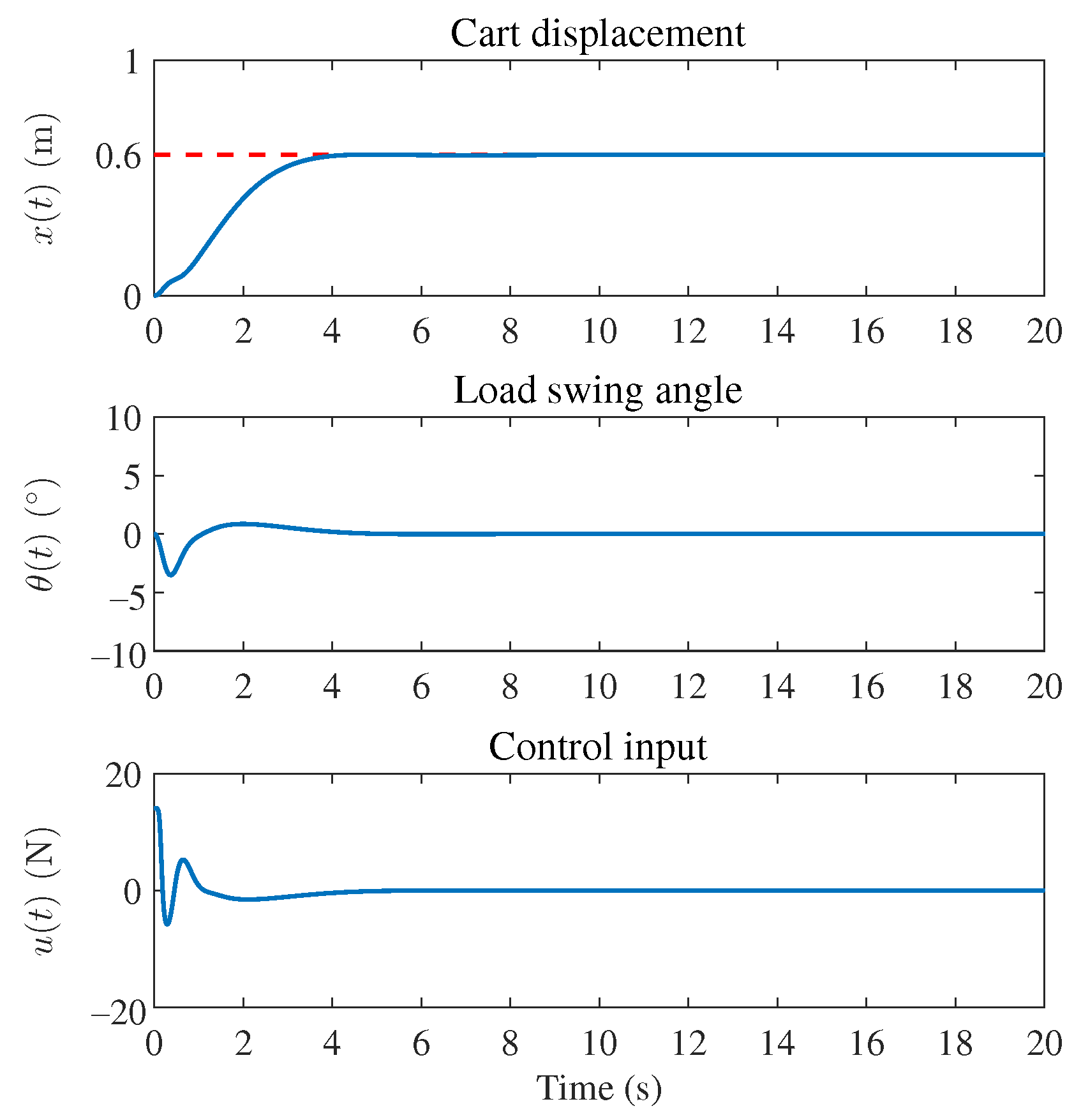
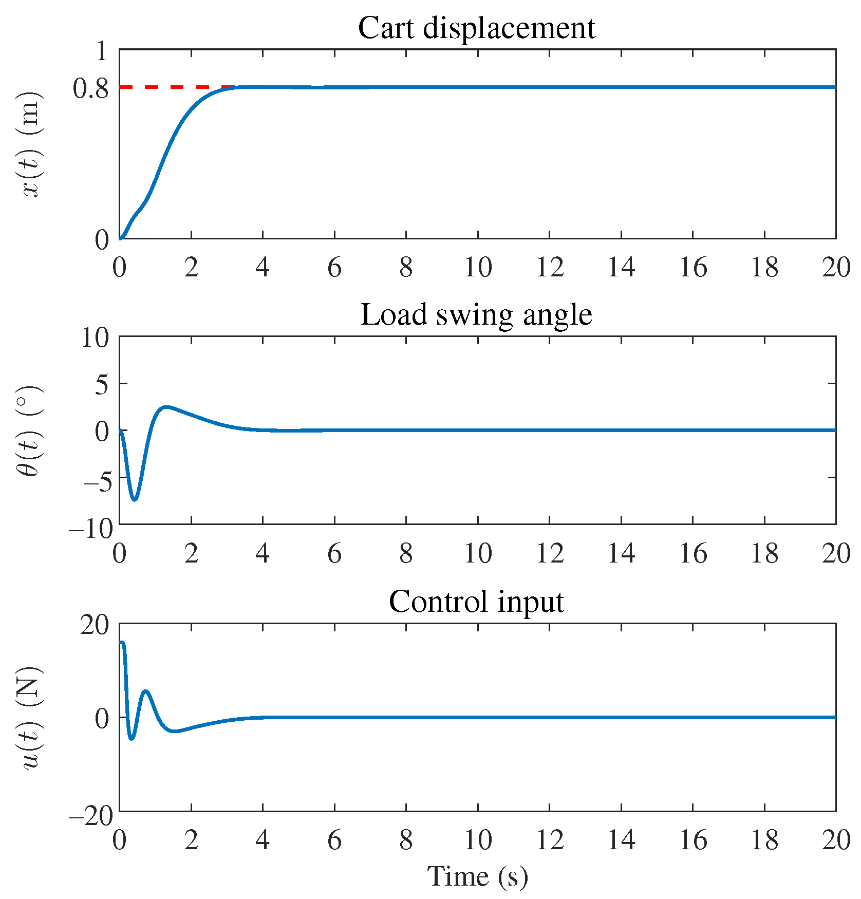
4. Simulation Results

In this section, in order to further demonstrate the regulation performance of the designed control approach and the estimation characteristic of the disturbance, a series of digital simulation tests are included by using MATLAB/Simulink. More precisely, we first verify the control performance of the proposed method under various system parameters and target locations. Then, external disturbances are considered to illustrate the robustness of the proposed method and an existing control method is chosen for a comparison study. The block diagram in Figure 2 depicts the entire control system to illustrate the proposed control framework.

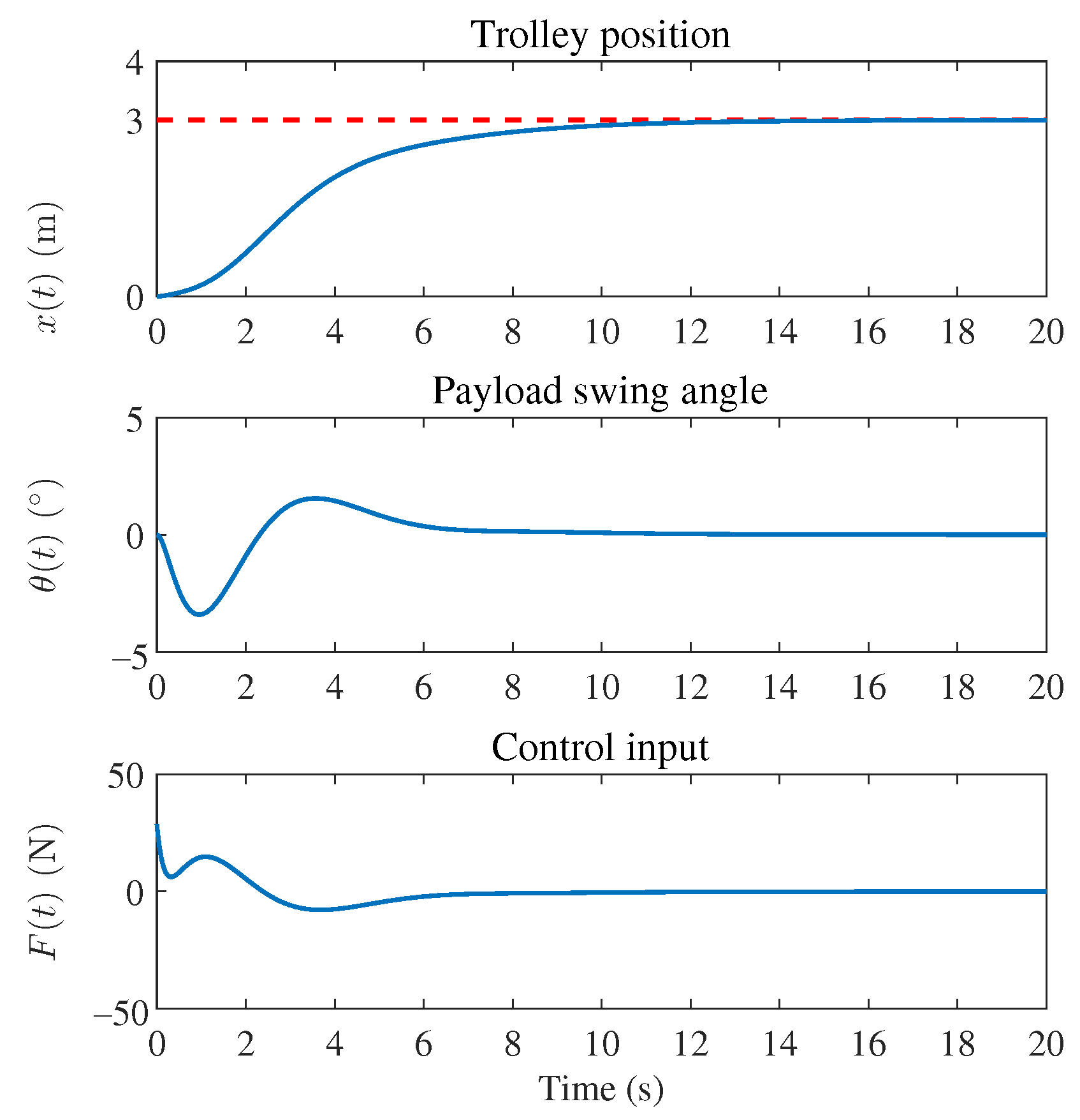
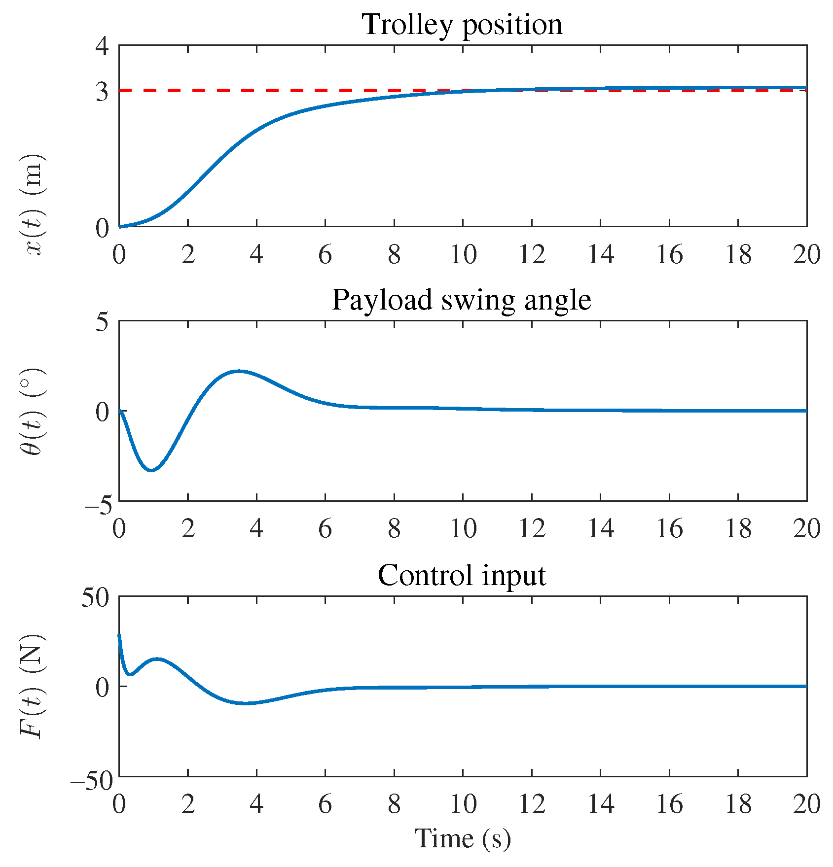
4.1. Effectiveness Verification

In this experiment, we ignore the external disturbances and will verify the effectiveness of the proposed method. First, the system parameters of the overhead crane are set as

$$\begin{array}{c}\hfill M=7\mathrm{kg},m=1\mathrm{kg},l=0.65\mathrm{m}.\end{array}$$

The control gains for the proposed method are

$$\begin{array}{c}\hfill k_1=-1.5,k_a=6,k_b=12.\end{array}$$

We set the initial condition as ${\left[x\left(0\right),\theta \left(0\right)\right]}^{\mathrm{T}}={\left[0,0\right]}^{\mathrm{T}}$ and the desired position as $x_d=0.6\mathrm{m}$. In order to verify the effectiveness of this controller against the system parameter changes and target position changes, the following two cases are considered:

Condition 1. 

The system parameters are adjusted to $M=9\mathrm{kg},m=2\mathrm{kg},l=0.75\mathrm{m}$.

Condition 2. 

We change the desired position from $x_d=0.6\mathrm{m}$ to $x_d=0.8\mathrm{m}$. We select the system parameters and control gains to be identical to the initial parameters.

The simulation results of the three cases are shown in Figure 3, Figure 4 and Figure 5, respectively. It can be seen from the results, under the proposed control method, that the trolley can finally be driven to the target point and there are almost no positioning errors. At the same time, the swing of the payload is suppressed and eliminated. The simulation results in Figure 4 and Figure 5 show that the proposed control method has good control performance for changes in the system parameters and target positions, which is beneficial to practical applications.

Remark 1. 

In practical applications, the motor actuates the trolley and an encoder embedded in the motor measures the trolley’s displacement. The angle encoder detects the payload swing. The velocity signals are obtained by applying numerical difference operations and low-pass filters to the position/angle signals. The motion control board with an I/O interface is used to collect data from the equipped encoder and transmit all the information to the host computer. The host computer generates control commands in real time through a calculation and sends them to the motor driver to control the motor.

4.2. Robustness Verification

In order to further evaluate the robustness of the proposed nonlinear control method, the following disturbances are introduced:

$$\begin{array}{cc}\hfill & d_1\left(t\right)=0.5sin\left(t\right)e^{-0.1t}\hfill \end{array}$$

(71)

$$\begin{array}{cc}\hfill & d_2\left(t\right)=tanh\left(\dot{x}\right)+0.5\left|\dot{x}\right|\dot{x}\hfill \end{array}$$

(72)

We choose the anti-swing control method (ASC) in [46] for the comparative study. The controller expression for the selected ASC method is as follows:

$$\begin{array}{cc}\hfill F=& (M+m{sin}^2\theta )\left\{-k_d[k_p(\dot{x}-\lambda sin\theta )-k_{E}cos\dot{\theta }]\right.\hfill \\ \hfill & \left.-\left[k_p(x-p_d-\lambda {\int }_0^{t}sin\theta \left(\tau \right)d\left(\tau \right))-k_{E}sin\theta \right]+\lambda \dot{\theta }cos\theta \right\}\hfill \\ \hfill & -msin\theta (gcos\theta +l{\dot{\theta }}^2)\hfill \end{array}$$

(73)

The controller gains of the ASC method are consistent with [46]:

$$\begin{array}{c}\hfill k_p=0.3,k_d=3.2,k_E=1.4,\lambda =1.8.\end{array}$$

In order to better compare the controller performance to verify the robustness of the proposed method, we select the system parameters to be consistent with those in [46].

$$\begin{array}{c}\hfill M=24\mathrm{kg},m=8\mathrm{kg},l=1.2\mathrm{m},x_d=3\mathrm{m}.\end{array}$$

The parameters of the proposed disturbance observer and the proposed controller gains are set to be

$$\begin{array}{cc}\hfill {\lambda }_1={\lambda }_2& ={\lambda }_3=1.3.\hfill \\ \hfill k_1=-9,& k_a=9,k_b=27.\hfill \end{array}$$

Figure 6, Figure 7, Figure 8 and Figure 9 record the results of the ASC method and the results of our proposed method, respectively. The simulation results demonstrate that our proposed method and the existing ASC methods can achieve trolley positioning and payload swing suppression under disturbance. By comparing Figure 8 with Figure 9, in the presence of disturbance $d_2$, both methods can achieve the positioning of the trolley within 10 s. The ASC method has positioning errors (about $6\mathrm{cm}$) that cannot be eliminated. However, the proposed controller has almost no positioning error and no residual payload swing. In addition, the proposed controller (maximum amplitude: 2.01 degrees in $d_1$ and 2.09 degrees in $d_2$) better suppresses and eliminates payload swings than the ASC method (maximum amplitude: 3.41 degrees in $d_1$ and 3.31 degrees in $d_2$), and the proposed method (about $2\mathrm{s}$) takes less time to eliminate the payload swing than the ASC method (about $6\mathrm{s}$). Moreover, the external disturbances are accurately estimated by the designed disturbance observer in a finite time. As shown by the simulation results, the performance of the proposed control method is superior to the existing ASC method.

5. Conclusions

In this article, a novel disturbance observer-based control method has been presented for the overhead crane system, which considers uncertain disturbances, input saturation and output feedback. First, we design a finite-time disturbance observer to estimate the uncertain disturbance. Then, a composite control method is introduced based on the new energy storage function and the designed disturbance observer. Compared with the existing full-state feedback control methods, from the practical and theoretical viewpoints, the proposed method in this paper takes three remarkable issues into consideration simultaneously: input saturation, output feedback and uncertain disturbances. The simulation results implemented in MATLAB/Simulink show that the proposed nonlinear disturbance observer can accurately and quickly estimate and compensate for different external disturbances. In addition, this method has good regulation control performance and strong robustness against uncertain disturbances. In future work, we will consider more practical issues, such as the inertia effect of the drive. Moreover, we plan to establish an experimental apparatus and evaluate the performance of the proposed approach through rigorous experiments, quantifying the experimental results with performance indicators.

References

1. Ortega, R.; Spong, M.; Gomez-Estern, F.; Blankenstein, G. Stabilization of a class of underactuated mechanical systems via interconnection and damping assignment. IEEE Trans. Autom. Control 2002, 47, 1218–1233. [Google Scholar] [CrossRef]
2. Franco, E.; Astolfi, A.; y Baena, F.R. Robust balancing control of flexible inverted-pendulum systems. Mech. Mach. Theory 2018, 130, 539–551. [Google Scholar] [CrossRef]
3. Li, E.; Liang, Z.Z.; Hou, Z.G.; Tan, M. Energy-based balance control approach to the ball and beam system. Int. J. Control 2009, 82, 981–992. [Google Scholar] [CrossRef]
4. Liang, X.; Fang, Y.; Sun, N.; Lin, H.; Zhao, X. Adaptive nonlinear hierarchical control for a rotorcraft transporting a cable-suspended payload. IEEE Trans. Syst. Man Cybern. Syst. 2019, 51, 4171–4182. [Google Scholar] [CrossRef]
5. Liang, X.; Fang, Y.; Sun, N.; Lin, H. A novel energy-coupling-based hierarchical control approach for unmanned quadrotor transportation systems. IEEE/ASME Trans. Mechatronics 2019, 24, 248–259. [Google Scholar] [CrossRef]
6. Aguilar-Ibáñez, C.; Sira-Ramírez, H.; Suárez-Castañón, M.S.; Martínez-Navarro, E.; Moreno-Armendariz, M.A. The trajectory tracking problem for an unmanned four-rotor system: Flatness-based approach. Int. J. Control 2012, 85, 69–77. [Google Scholar] [CrossRef]
7. Zhang, Y.; Li, S.; Liu, X. Adaptive near-optimal control of uncertain systems with application to underactuated surface vessels. IEEE Trans. Control Syst. Technol. 2017, 26, 1204–1218. [Google Scholar] [CrossRef]
8. Wen, S.; Chen, M.Z.; Zeng, Z.; Yu, X.; Huang, T. Fuzzy control for uncertain vehicle active suspension systems via dynamic sliding-mode approach. IEEE Trans. Syst. Man Cybern. Syst. 2016, 47, 24–32. [Google Scholar] [CrossRef]
9. Li, H.; Jing, X.; Karimi, H.R. Output-feedback-based H∞ control for vehicle suspension systems with control delay. IEEE Trans. Ind. Electron. 2013, 61, 436–446. [Google Scholar] [CrossRef]
10. Zhang, M. Finite-time model-free trajectory tracking control for overhead cranes subject to model uncertainties, parameter variations and external disturbances. Trans. Inst. Meas. Control 2019, 41, 3516–3525. [Google Scholar] [CrossRef]
11. Zhang, M.; Zhang, Y.; Cheng, X. Finite-time trajectory tracking control for overhead crane systems subject to unknown disturbances. IEEE Access 2019, 7, 55974–55982. [Google Scholar] [CrossRef]
12. Wu, X.; Xu, K.; Ma, M.; Ke, L. Output feedback control for an underactuated benchmark system with bounded torques. Asian J. Control 2021, 23, 1466–1475. [Google Scholar] [CrossRef]
13. Hu, R.; Han, L.; Huang, J. Stabilization control of underactuated cranes with guaranteed transient performance. In Proceedings of the 2018 Chinese Control And Decision Conference (CCDC), Shenyang, China, 9–11 June 2018; pp. 1358–1363. [Google Scholar]
14. Tang, R.; Huang, J. Control of bridge cranes with distributed-mass payloads under windy conditions. Mech. Syst. Signal Process. 2016, 72, 409–419. [Google Scholar] [CrossRef]
15. Maghsoudi, M.J.; Mohamed, Z.; Sudin, S.; Buyamin, S.; Jaafar, H.; Ahmad, S. An improved input shaping design for an efficient sway control of a nonlinear 3D overhead crane with friction. Mech. Syst. Signal Process. 2017, 92, 364–378. [Google Scholar] [CrossRef]
16. Sorensen, K.L.; Singhose, W.E. Command-induced vibration analysis using input shaping principles. Automatica 2008, 44, 2392–2397. [Google Scholar] [CrossRef]
17. Li, F.; Zhang, C.; Sun, B. A minimum-time motion online planning method for underactuated overhead crane systems. IEEE Access 2019, 7, 54586–54594. [Google Scholar] [CrossRef]
18. Sun, N.; Wu, Y.; Chen, H.; Fang, Y. An energy-optimal solution for transportation control of cranes with double pendulum dynamics: Design and experiments. Mech. Syst. Signal Process. 2018, 102, 87–101. [Google Scholar] [CrossRef]
19. Zhang, M.; Ma, X.; Chai, H.; Rong, X.; Tian, X.; Li, Y. A novel online motion planning method for double-pendulum overhead cranes. Nonlinear Dyn. 2016, 85, 1079–1090. [Google Scholar] [CrossRef]
20. Zhang, X.; Fang, Y.; Sun, N. Minimum-time trajectory planning for underactuated overhead crane systems with state and control constraints. IEEE Trans. Ind. Electron. 2014, 61, 6915–6925. [Google Scholar] [CrossRef]
21. Wu, X.; He, X.; Sun, N. An analytical trajectory planning method for underactuated overhead cranes with constraints. In Proceedings of the 33rd Chinese Control Conference, Nanjing, China, 28–30 July 2014; pp. 1966–1971. [Google Scholar]
22. Wu, X.; He, X. Nonlinear energy-based regulation control of three-dimensional overhead cranes. IEEE Trans. Autom. Sci. Eng. 2016, 14, 1297–1308. [Google Scholar] [CrossRef]
23. Sun, N.; Yang, T.; Chen, H.; Fang, Y.; Qian, Y. Adaptive anti-swing and positioning control for 4-DOF rotary cranes subject to uncertain/unknown parameters with hardware experiments. IEEE Trans. Syst. Man Cybern. Syst. 2017, 49, 1309–1321. [Google Scholar] [CrossRef]
24. Sun, N.; Fang, Y.; Wu, X. An enhanced coupling nonlinear control method for bridge cranes. IET Control Theory Appl. 2014, 8, 1215–1223. [Google Scholar] [CrossRef]
25. Sun, N.; Wu, Y.; Fang, Y.; Chen, H. Nonlinear antiswing control for crane systems with double-pendulum swing effects and uncertain parameters: Design and experiments. IEEE Trans. Autom. Sci. Eng. 2017, 15, 1413–1422. [Google Scholar] [CrossRef]
26. Zhang, M.; Ma, X.; Song, R.; Rong, X.; Tian, G.; Tian, X.; Li, Y. Adaptive proportional-derivative sliding mode control law with improved transient performance for underactuated overhead crane systems. IEEE/CAA J. Autom. Sin. 2018, 5, 683–690. [Google Scholar] [CrossRef]
27. Zhang, M.; Ma, X.; Rong, X.; Tian, X.; Li, Y. Adaptive tracking control for double-pendulum overhead cranes subject to tracking error limitation, parametric uncertainties and external disturbances. Mech. Syst. Signal Process. 2016, 76, 15–32. [Google Scholar] [CrossRef]
28. Sun, N.; Fang, Y.; Chen, H. Adaptive antiswing control for cranes in the presence of rail length constraints and uncertainties. Nonlinear Dyn. 2015, 81, 41–51. [Google Scholar] [CrossRef]
29. Sun, N.; Fang, Y.; Chen, H.; He, B. Adaptive nonlinear crane control with load hoisting/lowering and unknown parameters: Design and experiments. IEEE/ASME Trans. Mechatronics 2014, 20, 2107–2119. [Google Scholar] [CrossRef]
30. Wu, X.; Xu, K.; Lei, M.; He, X. Disturbance-compensation-based continuous sliding mode control for overhead cranes with disturbances. IEEE Trans. Autom. Sci. Eng. 2020, 17, 2182–2189. [Google Scholar] [CrossRef]
31. Zhang, M.; Zhang, Y.; Chen, H.; Cheng, X. Model-independent PD-SMC method with payload swing suppression for 3D overhead crane systems. Mech. Syst. Signal Process. 2019, 129, 381–393. [Google Scholar] [CrossRef]
32. Ouyang, H.; Wang, J.; Zhang, G.; Mei, L.; Deng, X. Novel adaptive hierarchical sliding mode control for trajectory tracking and load sway rejection in double-pendulum overhead cranes. IEEE Access 2019, 7, 10353–10361. [Google Scholar] [CrossRef]
33. Zhang, Z.; Wu, Y.; Huang, J. Differential-flatness-based finite-time anti-swing control of underactuated crane systems. Nonlinear Dyn. 2017, 87, 1749–1761. [Google Scholar] [CrossRef]
34. Smoczek, J.; Szpytko, J. Particle swarm optimization-based multivariable generalized predictive control for an overhead crane. IEEE/ASME Trans. Mechatronics 2016, 22, 258–268. [Google Scholar] [CrossRef]
35. Chen, H.; Fang, Y.; Sun, N. A swing constraint guaranteed MPC algorithm for underactuated overhead cranes. IEEE/ASME Trans. Mechatronics 2016, 21, 2543–2555. [Google Scholar] [CrossRef]
36. Wu, Z.; Xia, X.; Zhu, B. Model predictive control for improving operational efficiency of overhead cranes. Nonlinear Dyn. 2015, 79, 2639–2657. [Google Scholar] [CrossRef]
37. Jolevski, D.; Bego, O. Model predictive control of gantry/bridge crane with anti-sway algorithm. J. Mech. Sci. Technol. 2015, 29, 827–834. [Google Scholar] [CrossRef]
38. Drąg, Ł. Model of an artificial neural network for optimization of payload positioning in sea waves. Ocean Eng. 2016, 115, 123–134. [Google Scholar] [CrossRef]
39. Smoczek, J.; Szpytko, J. Evolutionary algorithm-based design of a fuzzy TBF predictive model and TSK fuzzy anti-sway crane control system. Eng. Appl. Artif. Intell. 2014, 28, 190–200. [Google Scholar] [CrossRef]
40. Lee, L.H.; Huang, P.H.; Shih, Y.C.; Chiang, T.C.; Chang, C.Y. Parallel neural network combined with sliding mode control in overhead crane control system. J. Vib. Control 2014, 20, 749–760. [Google Scholar] [CrossRef]
41. Sun, N.; Fang, Y.; Chen, H. A new antiswing control method for underactuated cranes with unmodeled uncertainties: Theoretical design and hardware experiments. IEEE Trans. Ind. Electron. 2014, 62, 453–465. [Google Scholar] [CrossRef]
42. Lee, H.H. Motion planning for three-dimensional overhead cranes with high-speed load hoisting. Int. J. Control 2005, 78, 875–886. [Google Scholar] [CrossRef]
43. Levant, A. Higher-order sliding modes, differentiation and output-feedback control. Int. J. Control 2003, 76, 924–941. [Google Scholar] [CrossRef]
44. Yang, J.; Su, J.; Li, S.; Yu, X. High-order mismatched disturbance compensation for motion control systems via a continuous dynamic sliding-mode approach. IEEE Trans. Ind. Inform. 2013, 10, 604–614. [Google Scholar] [CrossRef]
45. Yin, J.; Khoo, S.; Man, Z.; Yu, X. Finite-time stability and instability of stochastic nonlinear systems. Automatica 2011, 47, 2671–2677. [Google Scholar] [CrossRef]
46. Wu, X.; He, X.; Wang, M. A new anti-swing control law for overhead crane systems. In Proceedings of the 2014 9th IEEE Conference on Industrial Electronics and Applications, Hangzhou, China, 9–11 June 2014; pp. 678–683. [Google Scholar]
Figure 1. Schematic of the two-dimensional (2-D) overhead crane system.
Electronics 12 04474 g001
Figure 2. Block diagram of the simulation system.
Electronics 12 04474 g002
Figure 3. Simulation results of the proposed method with initial system parameters.
Electronics 12 04474 g003
Figure 4. Simulation results of the proposed method for Condition 1.
Electronics 12 04474 g004
Figure 5. Simulation results of the proposed method for Condition 2.
Electronics 12 04474 g005
Figure 6. Simulation results of the ASC method (73) with d 1 .
Electronics 12 04474 g006
Figure 7. Simulation results of the proposed method (42) with d 1 .
Electronics 12 04474 g007
Figure 8. Simulation results of the ASC method (73) with d 2 .
Electronics 12 04474 g008
Figure 9. Simulation results of the proposed method (42) with d 2 .
Electronics 12 04474 g009
Disclaimer/Publisher’s Note: The statements, opinions and data contained in all publications are solely those of the individual author(s) and contributor(s) and not of MDPI and/or the editor(s). MDPI and/or the editor(s) disclaim responsibility for any injury to people or property resulting from any ideas, methods, instructions or products referred to in the content.