Sinogram Upsampling via Sub-Riemannian Diffusion with Adaptive Weighting

Abstract

Computed tomography is a versatile imaging technique used to enable seeing internal structures of objects without opening or destroying them. This is possible through a process called tomographic reconstruction, which reconstructs images from projections of the object that are obtained by penetrating the object with beams of radiation, such as X-rays, from different angles. These projection data are often limited to low-resolution data in terms of projection angles. These limited or subsampled data make it difficult to obtain high-quality reconstruction results. Hence, upsampling projection data is necessary. In this paper, we propose a sinogram upsampling method via the sub-Riemannian diffusion process. We first lift the data into a feature space, and we fill in the missing angle parts by propagating information from the observed data to the missing parts. We observe that the sinogram with limited angle data has high directional dependency, and based on this observation, we suggest an adaptive weighting scheme to keep information propagating toward the missing regions. This adaptive weighting allows for diffusing toward the desired directions. The experimental results show the effectiveness of the proposed method in some scenarios regarding inpainting fine details, when compared to the existing model-based methods, such as Plug-and-Play and total generalized variation.

1. Introduction

Computed tomography (CT) is a computational imaging technique that uses radiation such as in X-rays to form cross-sectional images of the objects [1]. CT techniques are used in many applications, including industry, medical imaging and diagnosis [2,3,4,5]. The basic principle of CT is to measure the attenuation of radiation as it passes through the object, and the attenuation depends on the density of the object. By measuring the attenuation at multiple angles, it is possible to reconstruct the internal image of the object.

One of the challenges of CT imaging is that the sinogram, the raw data used to create the image, is often undersampled. This means that there are not enough measurements to accurately reconstruct the image. Sinogram upsampling is a technique that can be used to increase the resolution of the sinogram, which can lead to improved image quality. This is especially important for images of small objects or objects with complex shapes. Sinogram upsampling can also increase the contrast of CT images, which can make it easier to see subtle differences in the reconstructed images.

The sinogram upsampling problem can be considered as image inpainting because both problems involve filling in missing or corrupted data. In the case of sinogram upsampling, the missing data are the undersampled projection data, while in the case of image inpainting, the missing data are the pixels that have been corrupted or removed.

Among the image inpainting methods, there have been several works using sub-Riemannian diffusion, inspired by biological models of the primary visual cortex [6]. The primary visual cortex is a part of the brain that is responsible for processing visual information. It is organized into a hierarchy of layers, with each layer responding to different features of the visual image. The neurons of the primary visual cortex are organized into a hypercolumn structure, which allows V1 to process information from the entire visual field in a systematic and efficient way.

Sub-Riemannian diffusion methods for image inpainting lift an image into a feature space and propagate information from the observed pixels to the missing pixels [7,8,9]. The lifting process can be performed by, e.g., feature extractions from a Gabor transform [7] with different orientations. The information is propagated along a set of paths that are defined by the sub-Riemannian geometry of the primary visual cortex. The sub-Riemannian geometry is a way of measuring the distance between points in the visual space.

In this paper, we propose a sinogram upsampling method, inspired by computational models of the visual cortex. We lift the sinogram data to the Lie group of the rotation–translation SE(2) and fill in the missing projection values using the sub-Riemannian diffusion process. Then, the upsampled sinogram is obtained by projecting the lifted sinogram onto the original sinogram space. We adopt an adaptive weighting scheme during the diffusion process to account for the fact that the missing angles lead to vertical missing lines. In summary, the contributions of this paper are the following:

• We formulate the sinogram upsampling problem as a sub-Riemannian diffusion process.
• We propose an adaptive weighting scheme to exploit the characteristics of sinogram upsampling problems with respect to projection angles.
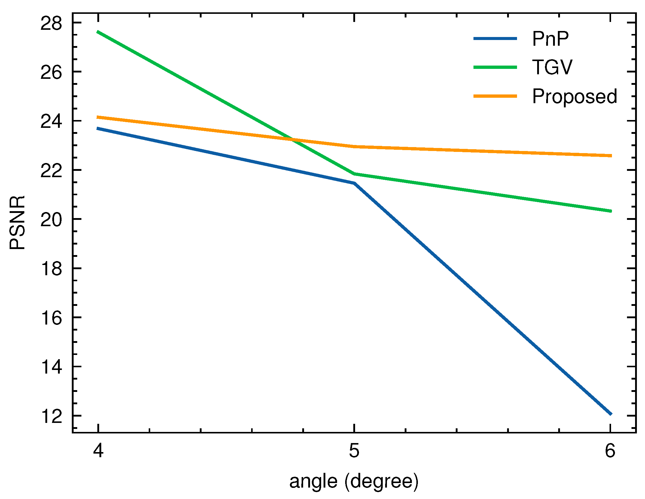
• The experimental results verify that the proposed method is effective for upsampling a sinogram with respect to projection angles, compared to some model-based methods.

This paper is organized as follows. In Section 2, we describe the related work on sinogram inpainting and sub-Riemannian diffusion for image processing. Section 3 explains the proposed method, and Section 4 demonstrates the numerical experiments and results with different scenarios. Section 5 discusses and concludes the paper.

2. Related Works

2.1. Sinogram Inpainting

A straightforward approach for sinogram inpainting is to regard a sinogram as an image and apply the image inpainting algorithm. This approach has been adopted in several works via variational methods [10] or interpolation [11].

Another approach is a data-driven inpainting approach in a supervised or unsupervised way. Lee et al. [12,13] employed convolutional neural networks patchwise to refine an initial guess obtained from interpolation. These methods belong to the category of supervised learning. Recently, there have been many attempts using unsupervised learning. Generative Adversarial Networks (GAN) [14] were adopted in [15]. To fill in large missing regions, an auto-encoder type called the context encoder was proposed for image inpainting [16] and this context encoder was used in [17] for sinogram inpainting. Valat et al. [18] incorporated the shape prior information into the GAN framework. One disadvantage of using a GAN is that it requires large computational resources and so it is difficult to scale to large data. Unlike the data-driven approach, our method does not require training data, often providing a more fast and reliable solution with greater interpretability than the data-driven approaches.

2.2. Image Processing via Sub-Riemannian Diffusion

Our method adopts the sub-Riemannian diffusion used in the image completion task, so we review such work. Sub-Riemannian diffusion is a type of diffusion process that is defined on a sub-Riemannian manifold. A sub-Riemannian manifold [19] is a manifold where the tangent space at each point is equipped with a non-degenerate inner product, but not all vectors in the tangent space are allowed to move [20]. The allowed vectors form a distribution, which is a subset of the tangent space. In 1989, Hoffman [21] considered the hypercolumn structure of V1 as a contact-bundle structure. It was developed further by several works, including [7,22], which proposed a mathematical model of the structure of V1 as the group of rotations and translations SE(2) and the receptive profiles as Gabor functions. This line of model is often called the Citti–Petitot–Sarti model, following the author names. This novel framework is extended to considering more features, such as multiscale or multifrequency [23]. Based on such a mathematical model of the visual cortex, sub-Riemnnian diffusion is employed for image completion problems [24,25,26,27,28] and for explaining visual illusions [29,30,31]. Unlike the existing sub-Riemannian diffusion work, we suggest an adaptive weighting scheme that is direction-dependent, which is suitable for sinogram inpainting.

3. Method

In this section, we propose an algorithm to upsample the sinogram with respect to projection angles. Before introducing the proposed method, we review the data acquisition process in CT imaging. In CT, the data acquisition process can be modeled as a process called Radon transform. The Radon transform of an image $I:\Omega \subset {\mathbb{R}}^2\to \mathbb{R}$ maps the image into a measurement space, defined as:

$$\begin{array}{cc}\hfill p(r,s)& =\mathcal{R}\left[I\right]\hfill \\ \hfill & ={\int }_{-\infty }^{\infty }{\int }_{-\infty }^{\infty }I(x,y)\delta (xcosr+ysinr-s)dxdy\hfill \end{array}$$

(1)

where s represents the position of the detector and r is the rotation angle. This measurement is called projection and the projection value $p(r,s)$ represents the line integral of I along the line: $xcosr+ysinr-s$.

From this setting, sinogram upsampling aims to upsample signals with respect to projection angles r. For this problem, the proposed method consists of three stages: the lifting stage, diffusion stage and projection stage, summarized in Algorithm 1.

Algorithm 1 Sinogram upsampling method

1: Input: Sinogram data p, projection angles M to be upsampled 2: Lifting the sinogram to obtain O (Section 3.1) 3: Sub-Riemannian diffusion (Section 3.2) 4: Projection of the lifted sinogram to the original space (Section 3.3) 5: Output: Upsampled sinogram

3.1. Lifting

We lift the sinogram data to the lifting space $M={\mathbb{R}}^2\times [0,2\pi )$ by extracting the orientation features by Gabor filters. The Gabor function G is defined as

$$G(r,s,\theta ):=\frac{1}{2{\sigma }^2}{\mathrm{e}}^{-i\left(f(-rsin\theta +scos\theta )-\varphi \right)}{\mathrm{e}}^{-\frac{r^2+s^2}{2{\sigma }^2}}$$

(2)

where $\varphi$ is a phase component, f is the spatial frequency and $\sigma$ is the scaling parameter. In the experiments, we set $\varphi$ to 0. The lifted sinogram F is obtained by the convolution of G and the sinogram data p as follows:

$$F(r,s,\theta )=\int G(r-r^{\prime },s-s^{\prime },\theta )p(r^{\prime },s^{\prime })d{r}^{\prime }d{s}^{\prime }.$$

(3)

3.2. Sub-Riemannian Diffusion

From the lifted sinogram, the goal is two-fold: (i) we propagate the information from the observed projections to the missing projections in the unknown projection angles; (ii) we denoise the lifted sinogram in an anisotropic way. To achieve this goal, we employ the sub-Riemannian diffusion process, where smoothing can be imposed in some directions more than others.

To consider connections in the geometry M of the lifting space, sub-Riemannian geometry considers a subbundle called the horizontal vector fields $HM$ of the tangent bundle $TM$. A subbundle of a tangent bundle is a proper subset of the tangent bundle, which is itself a vector bundle. In our rotation–translation lifting space M, we consider the following horizontal vector fields:

$$\begin{array}{cc}\hfill X_1& =cos\theta {\partial }_r+sin\theta {\partial }_s,\hfill \end{array}$$

(4)

$$\begin{array}{cc}\hfill X_2& ={\partial }_{\theta }.\hfill \end{array}$$

(5)

Note that for each point $p\in M$,

$$span\{X_1,X_2\}{|}_p\subset T_{p}M,$$

(6)

but the horizontal vector fields have the bracket-generating property such that

$$span\{X_1,X_2,[X_1,X_2]\}{|}_p=T_{p}M,$$

(7)

where $[X_1,X_2]=sin\theta {\partial }_r-cos\theta {\partial }_s$.

From the horizontal vector fields, we can take the corresponding integral curves. An integral curve of a vector field X is a curve $\gamma :[0,1]\to M$ such that ${\gamma }^{\prime }\left(t\right)=V_{\gamma \left(t\right)}\mathrm{for}\mathrm{all}t\in J$ [32]. Integral curves of horizontal vector fields are called horizontal integral curves, and following these curves, we can fill in the missing parts of the sinogram. Citti and Sarti [7] consider the SE(2) sub-Riemannian diffusion operator $X_1^2+\beta X_2^2$.

3.2.1. Adaptive Weighting

In this paper, we focus on the sinogram upsampling with respect to projection angles. We observe that the information should be less propagated from the vertical directions on the missing regions. With this motivation, we suggest using the diffusion operator with adaptive weighting, as follows:

$$\mathcal{L}=\alpha (r,s,\theta )X_1^2{{|}_{(r,s,\theta )}+\beta X_2^2|}_{(r,s,\theta )}$$

(8)

where we choose the weighting parameter $\alpha$ as

$$\alpha (r,s,\theta )={\mathbf{1}}_A(r,s,\theta )exp(-{\alpha }_0{sin}^2\theta )+(1-{\mathbf{1}}_A(r,s,\theta )),$$

(9)

where A is the set of missing positions in the sinogram and $1_A(r,s,\theta )$ is the indicator function, defined as

$${\mathbf{1}}_A\left(x\right)=\left\{\begin{array}{cc}1\hfill & \mathrm{if}x\in A\hfill \\ 0\hfill & \mathrm{if}x\notin A\hfill \end{array}\right..$$

(10)

The motivation of this choice is to diffuse less along the vertical directions on the missing positions. Another weighting parameter $\beta$ is chosen as $T/\left(RS\right)$, where T is the number of lifting angles $\theta$’s, R is the number of projection angles r and S is the number of detector pixels s.

From the sub-Riemannian diffusion operator, we update the lifted sinogram P as follows:

$${\partial }_{t}P=\mathcal{L}P$$

(11)

where t denotes the time variable.

3.2.2. Discretization

To discretize the diffusion process (11), we consider its discrete version:

$$P^{t+1}=P^t+(\Delta t)\mathcal{L}{P}^t$$

(12)

where $\Delta t$ is the step size. We also need to discretize the operators $X_1^2$ and $X_2^2$. We discretize the lifted space, and for simplicity, the intervals $\Delta r$ and $\Delta s$ are set to 1. For the Gabor filter angle $\theta$, we introduce the index i such that we are given $\{{\theta }_1,{\theta }_2,\cdots ,{\theta }_i,\cdots ,{\theta }_T\}$, with T the number of Gabor filter angles during the lifting. From this setting, we adopt a second-order centered difference approximation of derivatives as follows:

$$\begin{array}{cc}\hfill X_1^{2}P& =P(r+cos{\theta }_i,s+sin{\theta }_i,{\theta }_i)-2P(r,s,{\theta }_i)+P(r-cos{\theta }_i,s-sin{\theta }_i,{\theta }_i)\hfill \end{array}$$

(13)

$$\begin{array}{cc}\hfill X_2^{2}P& =\delta (P(r,s,{\theta }_{i+1})-2P(r,s,{\theta }_i)+P(r,s,{\theta }_{i-1}))\hfill \end{array}$$

(14)

where we consider $\delta =1$ in our experiments for numerical stability when considering a large number of angles in the Gabor filters. Note that the values of P are available on the uniform grid. Hence, to evaluate $P(r+cos{\theta }_i,s+sin{\theta }_i,{\theta }_i)$ and $P(r-cos{\theta }_i,s-sin{\theta }_i,{\theta }_i)$, we need to interpolate, and we use B-spline interpolation [33] from the values on the uniform grid.

3.3. Projection

After finishing the diffusion process, we need to project back the lifted sinogram to the original sinogram space. We adopt the summation projection as follows:

$$p(r,s)=\mid \sum _{i}P(r,s,{\theta }_i)\mid ,$$

(15)

where the absolute operator is taken to convert complex values to real values. An alternative way for lifting and projection is to use cake wavelets [34,35], which are invertible. However, we observe that due to the dependency on Fourier transform, cake wavelets have some numerical issues when we have vertical missing regions.

4. Results

In this section, we perform the numerical experiments to test the proposed method.

4.1. Test Dataset

We consider three phantom images, as shown in the first row of Figure 1. From the phantom images, we generate ground-truth sinograms by Radon transform (1) with 180 projection angles and 363 detector pixels, visualized in the third row. From these ground-truth sinograms, we remove 44, 88 or 132 projection angles and impose Gaussian noise with variance, 0.0001. The goal of the experiments is to upsample and denoise the undersampled noisy sinogram data.

4.2. Comparison Methods

In imaging applications, many problems can be formulated as optimizing a cost function, which consists of a data fidelity term and regularization term. To compare our method, we formulate the sinogram upsampling problem as a variational imaging problem as follows:

$$\underset{p}{min}{\parallel p_{\mathrm{d}ata}-\mathcal{A}\left(p\right)\parallel }_2^2+\lambda Reg\left(p\right)$$

(16)

where $\mathcal{A}$ is the undersampling operator to map an upsampled sinogram p to the original data space. In Equation (16), the first term is the data fidelity term, the second term Reg is the regularization term and the parameter $\lambda$ controls the trade-off between the two terms.

Plug-and-Play (PnP) with median filtering. Some first-order optimization algorithms [36] alternatively optimize the two terms. When optimizing (16), minimizing the regularization term often corresponds to a denoising problem. To take advantage of the state-of-the-art denoising methods, the Plug-and-Play (PnP) scheme [37] provides a flexible framework to replace the denoising step with sophisticated denoising schemes. In our experiments, we use median filtering as a denoiser. We use Half-Quadratic Splitting [38] as an optimizer.

Total generalized variation (TGV). One of the most popular image priors is total variation regularization [39], which was generalized by Bredies et al. [40] in 2010 as total generalized variation (TGV). Specifically, TGV aims to optimize

$$\underset{p}{min}\parallel p_{\mathrm{d}ata}{-\mathcal{A}\left(p\right)\parallel }_2^2+{\lambda }_1{\parallel r\parallel }_{1,2}+{\lambda }_2{\parallel J(\nabla p-r)\parallel }_{1,F}$$

(17)

where r is an auxiliary variable, ∇ is the discrete gradient operator, J is the Jacobian operator and ${\parallel ·\parallel }_{1,F}$. We use the Alternating Direction Method of Multipliers (ADMM) [41] as an optimizer. We use the deepinv library [42] for the implementation of PnP and TGV.

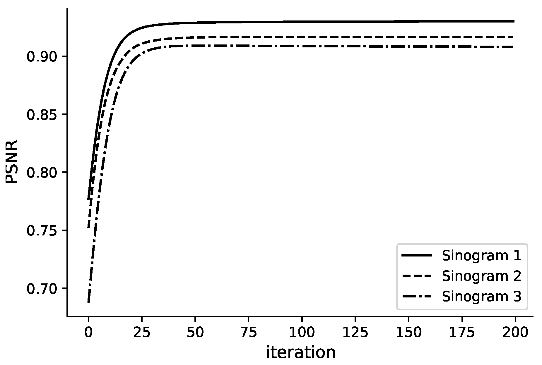
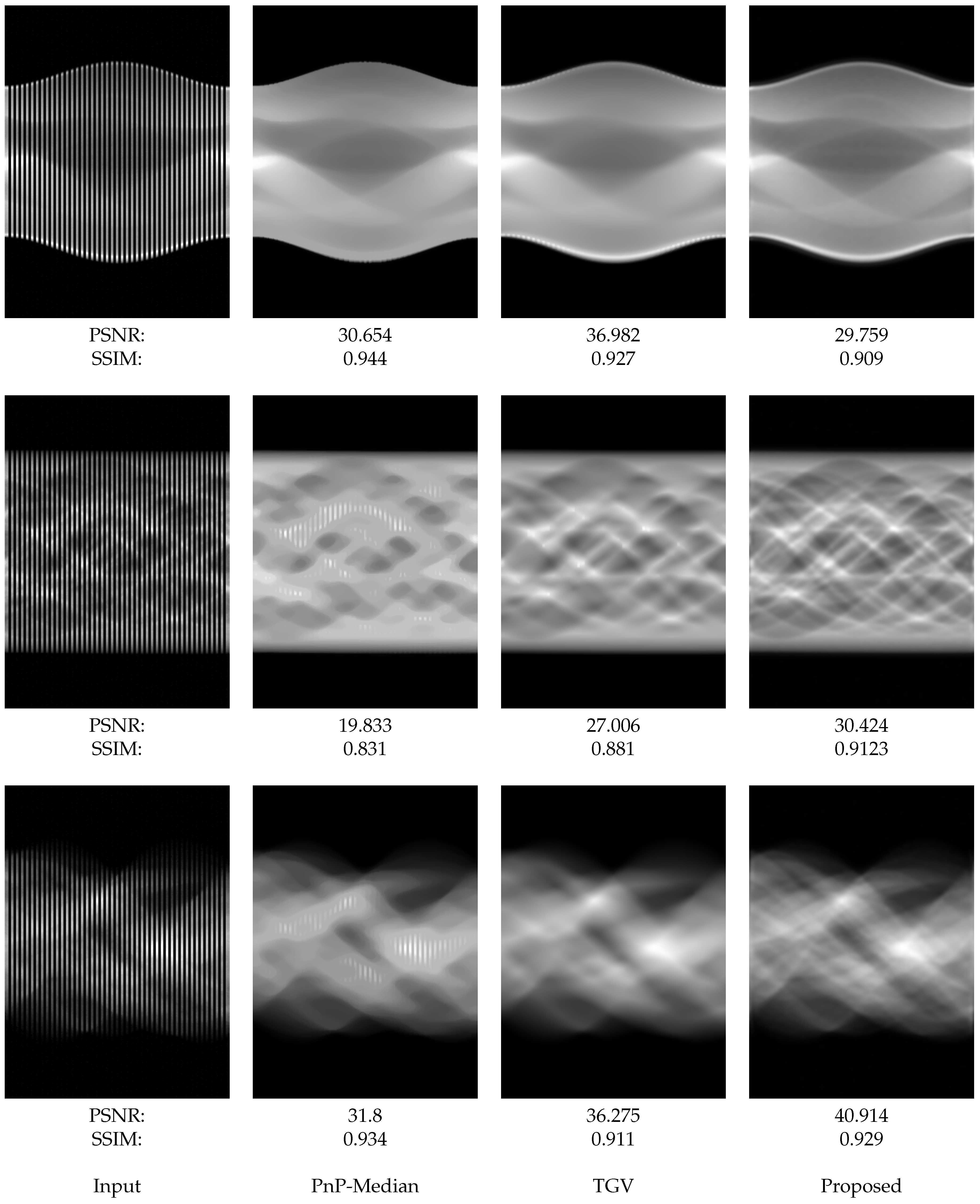
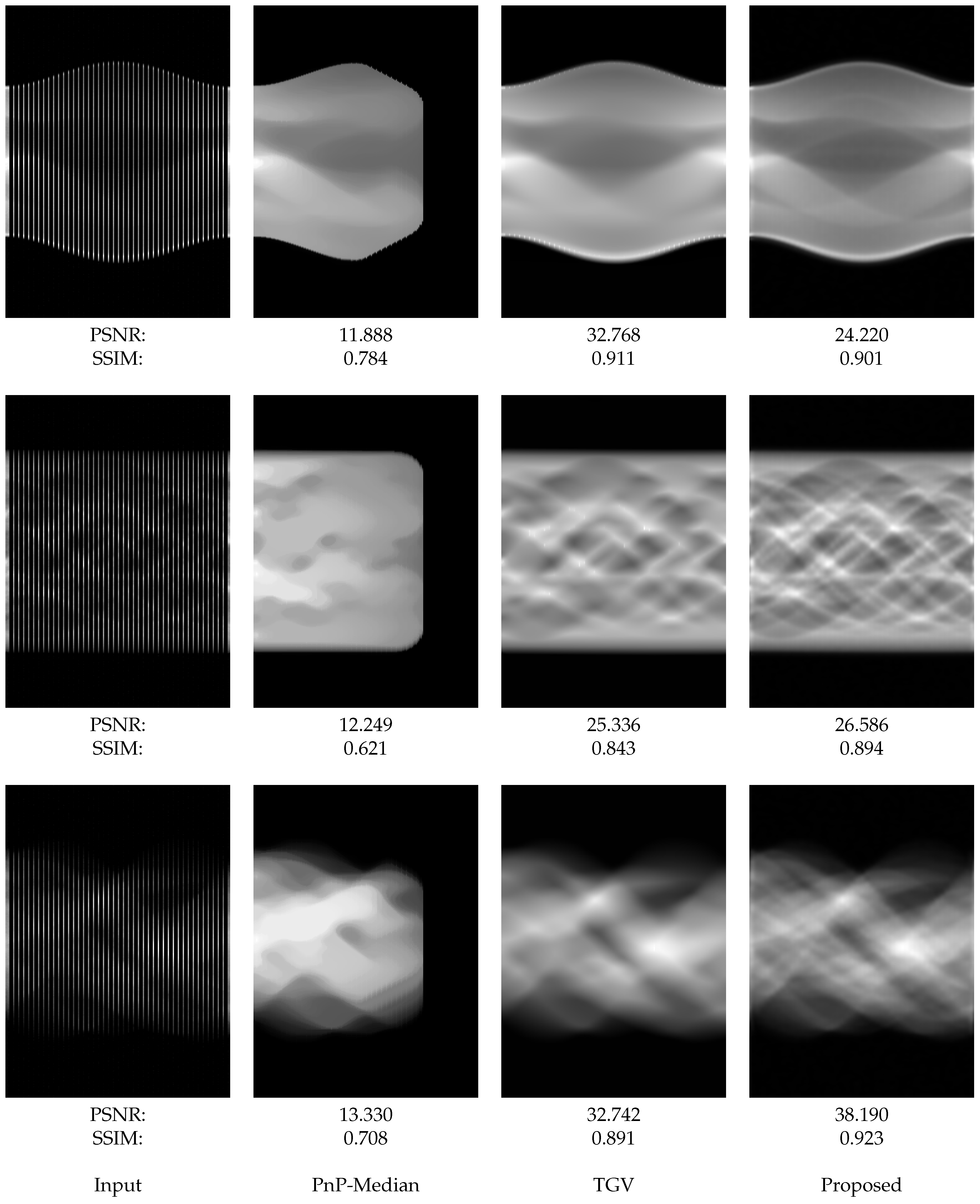
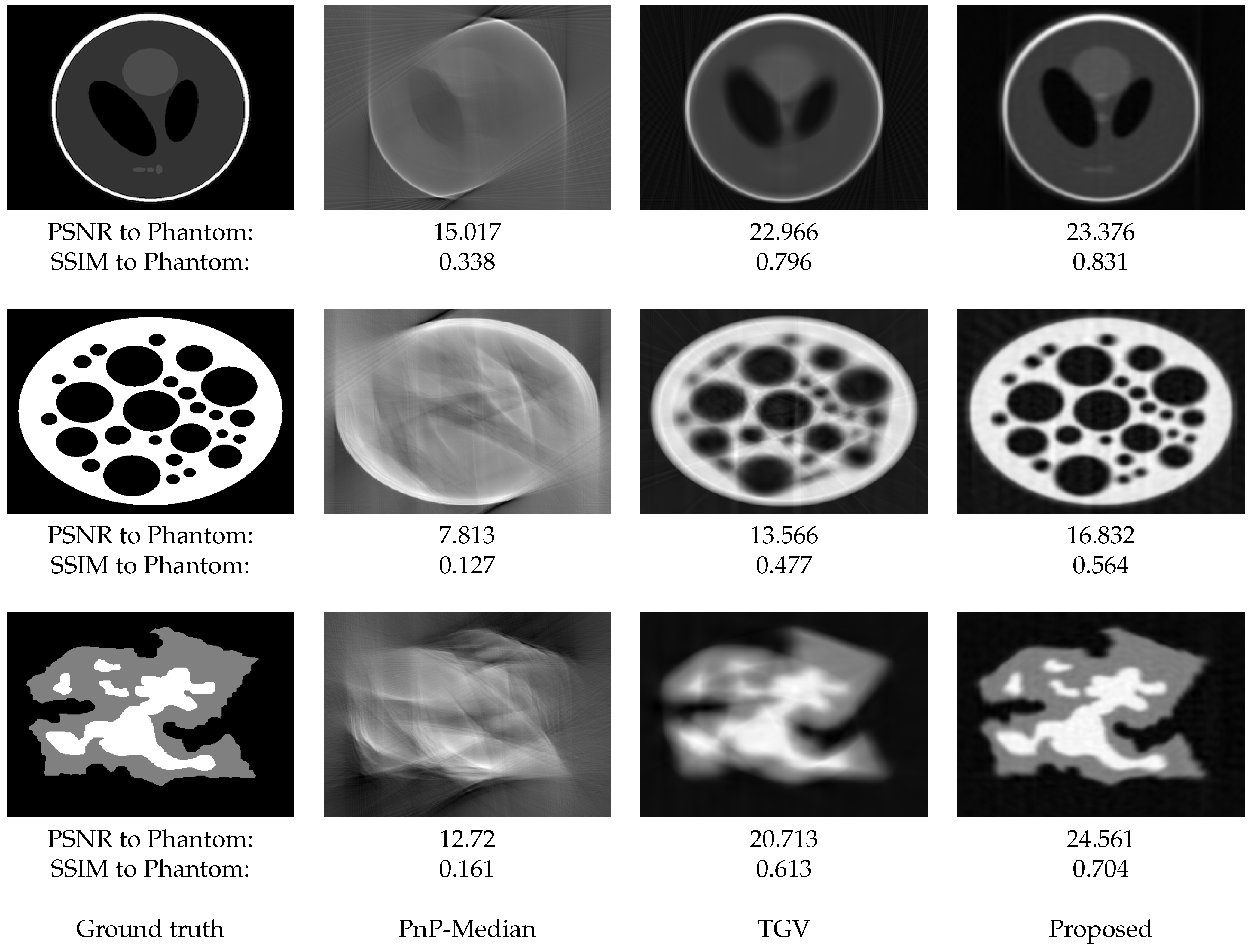
4.3. Experimental Results

We use the same parameters throughout the numerical experiments as follows: the step size is $\Delta t=0.5$, the weighting hyperparameter is ${\alpha }_0=10$ and the number of iterations is 200.

In the first experiment, we removed 44 projection angles, and the goal was to upsample 44 projection angles. Figure 2 shows the convergence behavior for Sinograms 1, 2 and 3 during the iteration. Figure 3 shows the qualitative upsampling results from the noisy sinogram data from the different methods. The first row shows the results for Sinogram 1. The PnP method misses the top and bottom boundaries of the sinogram. Overall, the proposed method estimates fine details well, but some artifacts are observed near the boundary of the sinogram. The second row shows the results for Sinogram 2 and the proposed method can also estimate fine structures well and shows fewer artifacts near the sinogram border, compared to that of Sinogram 1. This is because the contrast is small in Sinogram 1, but in Sinogram 2, due to the large contrast, we observe some blurring effects in our results.

Figure 4 presents the results of upsampling 88 projection angles from noisy sinograms. PnP with median filters yields some artifacts due to large missing areas. TGV produces typically blurry results, while the proposed method produces overall good results.

As shown in Figure 5, the numerical results are demonstrated to upsample 132 projection angles from noisy sinograms. PnP with median filters shows severe artifacts on the right part due to large missing areas. TGV again produces blurry results to fill in the large missing areas. On the other hand, the proposed method overall captures fine details better than TGV. Figure 6 shows the reconstructed images from the upsampled sinograms in Figure 5. It is clear from the reconstructed images that the the proposed method reconstructs fine details well with better contrasts, which is a distinct advantage of the proposed method.

Table 1. Quantitative comparison of sinogram upsampling methods. The best results are in bold.

Sinogram	Upsampled Angles	Metric	PnP-Median	TGV	Proposed
Sinogram 1	44	PSNR	32.588	39.615	33.591
		SSIM	0.972	0.935	0.907
Sinogram 2	44	PSNR	21.159	27.249	34.933
		SSIM	0.913	0.899	0.917
Sinogram 3	44	PSNR	36.573	38.818	42.215
		SSIM	0.974	0.919	0.930
Sinogram 1	88	PSNR	30.654	36.982	29.759
		SSIM	0.944	0.927	0.909
Sinogram 2	88	PSNR	19.833	27.006	30.424
		SSIM	0.831	0.881	0.9123
Sinogram 3	88	PSNR	31.8	36.275	40.914
		SSIM	0.934	0.911	0.929
Sinogram 1	132	PSNR	11.888	32.768	24.220
		SSIM	0.784	0.911	0.901
Sinogram 2	132	PSNR	12.249	25.336	26.586
		SSIM	0.621	0.843	0.894
Sinogram 3	132	PSNR	13.330	32.742	38.190
		SSIM	0.708	0.891	0.923

provides the quantitative comparison in terms of the Peak Signal-to-Noise Ratio (PSNR) and the Structural Similarity Index Measure (SSIM) [43]. Interestingly, PnP with median filtering often gives the best results in terms of the SSIM but shows poor performance in terms of the PSNR. For Sinogram 2, the proposed method shows the best performance. For Sinogram 1, TGV presents the best performance in terms of the PSNR, compared to the proposed method.

Figure 7 shows the quantitative results with respect to the different projection angles available. Specifically, the sinogram data are available on every 4, 5 or 6 angles among the 180 angles. Figure 8 shows the corresponding reconstruction images. In particular, the proposed method is shown to capture small details in the bottom of the objects.

Table 2. Comparison of computation time when upsampling 88 angles. The computation time in the proposed method is divided into three parts of lifting, diffusion and projection.

	PnP-Median	TGV	Proposed
Computational time (in seconds)	0.26	27.82	3.11 = 1.3 + 1.7 + 0.11

provides the computational efficiency between the proposed method and other methods. We use a Linux server containing an NVIDIA GeForce RTX 4090 card. This GPU is used for PnP-Median and TGV. For the proposed method, we use a CPU for the lifting stage and a GPU for the diffusion and projection steps. Hence, there is room for improving the computational speed by parallelizing the lifting step.

Lastly, we test the proposed method on the Walnut dataset provided by [44]. This object is scanned by microCT with an exposure time of 1000 ms, an acceleration voltage of 40 kV and a current of 1 mA in the X-ray tube. The sinogram data have 180 projection angles. We preprocess the sinogram data for converting the fan-beam geometry to parallel-beam geometry, because the proposed method is currently developed for parallel-beam geometry. We further normalize the range of data lying in between 0 and 1 and extract 256 detector pixels. Because they are real data, there is no exact ground truth, but a reference image is provided from [44]. Figure 9 shows the reconstruction results after upsampling 44 missing angles. The first column shows the reference image. The 2nd, 3rd and 4th columns show the reconstruction results after upsampling via Plug-and-Play with the median filter, total generalized variation and the proposed method, respectively.

5. Discussion and Conclusions

In this paper, we propose a sinogram upsampling method via sub-Riemannian diffusion. The proposed method first lifts the sinogram into a rotation-and-translation space. The lifted sinogram has many missing parts that are to be filled in by the diffusion process on the lifted space. After the diffusion process, it is projected back to the original sinogram space. In the diffusion process, we adopt a direction-dependent weighting scheme to keep noisy information propagating toward the missing regions. The numerical experiments on the simulated phantom and Walnut dataset [44] show the effectiveness of the proposed method, compared to the existing Plug-and-Play and total generalized variation work. The proposed method can also be applied to sinogram inpainting with respect to detector pixels, as well as projection angles. In this case, we can consider another adaptive weighting procedure and we leave it as future work.

A drawback of the proposed method is that lifting and projection are not invertible. For example, a clever transformation known as the cake wavelets lift [34,35] can be used to give invertible procedures. The idea of cake wavelets is to divide the frequency space into small parts, where each part can refer to some orientations. To these small parts, the inverse Fourier transforms are applied, and the real parts can serve as line detectors and the imaginary parts can serve as edge detectors with a specific orientation. However, due to the dependency on fast Fourier transform, applying that lift to sinogram upsampling with vertical missing regions yields some numerical artifacts. We leave it as future work to make lifting and projection invertible with numerical stability.

Further future work would be to extend the proposed method to sinogram inpainting. In this paper, we deal with sinogram data where projection angles are available for at least every 2 or up to 6 degrees. It has many applications, such as diagnosis or security applications. Another important problem, the so-called limited angle problem, considers missing angles in a specific range, such as −20 degrees to 20 degrees. The proposed method is not designed to deal with such limited angle data, as there is no information to propagate from the limited range. However, the data-driven approach using deep learning can be combined with the proposed method to tackle this problem. We leave it as future work.

References

1. Buzug, T.M. Computed Tomography: From Photon Statistics to Modern Cone-Beam CT; Springer: Berlin/Heidelberg, Germany, 2009. [Google Scholar]
2. Huang, D.; Swanson, E.A.; Lin, C.P.; Schuman, J.S.; Stinson, W.G.; Chang, W.; Hee, M.R.; Flotte, T.; Gregory, K.; Puliafito, C.A. Optical Coherence Tomography. Science 1991, 254, 1178–1181. [Google Scholar] [CrossRef] [PubMed]
3. Drexler, W.; Liu, M.; Kumar, A.; Kamali, T.; Unterhuber, A.; Leitgeb, R.A. Optical Coherence Tomography Today: Speed, Contrast, and Multimodality. J. Biomed. Opt. 2014, 19, 071412. [Google Scholar] [CrossRef] [PubMed]
4. Cogliati, A.; Canavesi, C.; Hayes, A.; Tankam, P.; Duma, V.F.; Santhanam, A.; Thompson, K.P.; Rolland, J.P. MEMS-based Handheld Scanning Probe with Pre-Shaped Input Signals for Distortion-Free Images in Gabor-domain Optical Coherence Microscopy. Opt. Express 2016, 24, 13365–13374. [Google Scholar] [CrossRef] [PubMed]
5. Măroiu, A.C.; Sinescu, C.; Duma, V.F.; Topală, F.; Jivănescu, A.; Popovici, P.M.; Tudor, A.; Romînu, M. Micro-CT and Microscopy Study of Internal and Marginal Gap to Tooth Surface of Crenelated versus Conventional Dental Indirect Veneers. Medicina 2021, 57, 772. [Google Scholar] [CrossRef] [PubMed]
6. Hubel, D.H.; Wiesel, T.N. Receptive Fields of Single Neurones in the Cat’s Striate Cortex. J. Physiol. 1959, 148, 574–591. [Google Scholar] [CrossRef]
7. Citti, G.; Sarti, A. A Cortical Based Model of Perceptual Completion in the Roto-Translation Space. J. Math. Imaging Vis. 2006, 24, 307–326. [Google Scholar] [CrossRef]
8. Boscain, U.; Gauthier, J.; Prandi, D. Image Inpainting via a Control-Theoretical Model of Human Vision. In Proceedings of the 2018 IEEE 14th International Conference on Control and Automation (ICCA), Anchorage, AK, USA, 12–15 June 2018; pp. 963–968. [Google Scholar]
9. Baspinar, E.; Sarti, A.; Citti, G. A Sub-Riemannian Model of the Visual Cortex with Frequency and Phase. J. Math. Neurosci. 2020, 10, 11. [Google Scholar] [CrossRef]
10. Kostler, H.; Prummer, M.; Rude, U.; Hornegger, J. Adaptive Variational Sinogram Interpolation of Sparsely Sampled CT Data. In Proceedings of the 18th International Conference on Pattern Recognition (ICPR’06), Hong Kong, China, 20–24 August 2006; Volume 3, pp. 778–781. [Google Scholar]
11. Benammar, A.; Allag, A.; Drai, R.; Yahi, M.; Boutkedjirt, T. Sinogram Interpolation Method for Limited-Angle Tomography. In Proceedings of the 2019 International Conference on Advanced Electrical Engineering (ICAEE), Algiers, Algeria, 19–21 November 2019; pp. 1–5. [Google Scholar]
12. Lee, H.; Lee, J.; Cho, S. View-Interpolation of Sparsely Sampled Sinogram Using Convolutional Neural Network. Med. Imaging 2017, 10133, 1013328. [Google Scholar]
13. Lee, H.; Lee, J.; Kim, H.; Cho, B.; Cho, S. Deep-Neural-Network-Based Sinogram Synthesis for Sparse-View CT Image Reconstruction. IEEE Trans. Radiat. Plasma Med. Sci. 2018, 3, 109–119. [Google Scholar] [CrossRef]
14. Goodfellow, I.; Pouget-Abadie, J.; Mirza, M.; Xu, B.; Warde-Farley, D.; Ozair, S.; Courville, A.; Bengio, Y. Generative Adversarial Nets. In Advances in Neural Information Processing Systems; The MIT Press: Cambridge, MA, USA, 2014; pp. 2672–2680. [Google Scholar]
15. Anirudh, R.; Kim, H.; Thiagarajan, J.J.; Mohan, K.A.; Champley, K.; Bremer, T. Lose the Views: Limited Angle CT Reconstruction via Implicit Sinogram Completion. In Proceedings of the 2018 IEEE/CVF Conference on Computer Vision and Pattern Recognition, Salt Lake City, UT, USA, 18–23 June 2018; pp. 6343–6352. [Google Scholar]
16. Pathak, D.; Krahenbuhl, P.; Donahue, J.; Darrell, T.; Efros, A.A. Context Encoders: Feature Learning by Inpainting. In Proceedings of the 2016 IEEE Conference on Computer Vision and Pattern Recognition (CVPR), Las Vegas, NV, USA, 27–30 June 2016; pp. 2536–2544. [Google Scholar]
17. Yoo, S.; Yang, X.; Wolfman, M.; Gursoy, D.; Katsaggelos, A.K. Sinogram Image Completion for Limited Angle Tomography with Generative Adversarial Networks. In Proceedings of the 2019 IEEE International Conference on Image Processing (ICIP), Taipei, Taiwan, 22–25 September 2019; pp. 1252–1256. [Google Scholar]
18. Valat, E.; Farrahi, K.; Blumensath, T. Sinogram Inpainting with Generative Adversarial Networks and Shape Priors. Tomography 2023, 9, 1137–1152. [Google Scholar] [CrossRef]
19. Agrachev, A.; Barilari, D.; Boscain, U. A Comprehensive Introduction to Sub-Riemannian Geometry; Cambridge Studies in Advanced Mathematics; Cambridge University Press: Cambridge, UK, 2019. [Google Scholar]
20. Agrachev, A.; Barilari, D.; Boscain, U. Introduction to Geodesics in Sub-Riemannian Geometry. In EMS Series of Lectures in Mathematics, 1st ed.; Barilari, D., Boscain, U., Sigalotti, M., Eds.; EMS Press: Helsinki, Finland, 2016; pp. 1–83. [Google Scholar]
21. Hoffman, W.C. The Visual Cortex Is a Contact Bundle. Appl. Math. Comput. 1989, 32, 137–167. [Google Scholar] [CrossRef]
22. Petitot, J.; Tondut, Y. Vers une neurogéométrie. Fibrations corticales, structures de contact et contours subjectifs modaux. Math. Inform. Sci. Hum. 1999, 145, 5–101. [Google Scholar] [CrossRef]
23. Baspinar, E. Multi-Frequency Image Completion via a Biologically-Inspired Sub-Riemannian Model with Frequency and Phase. J. Imaging 2021, 7, 271. [Google Scholar] [CrossRef] [PubMed]
24. Sanguinetti, G.; Citti, G.; Sarti, A. Image Completion Using a Diffusion Driven Mean Curvature Flow in a Sub-Riemannian Space. In Proceedings of the Third International Conference on Computer Vision Theory and Applications, Funchal, Madeira, Portugal, 22–25 January 2008; pp. 46–53. [Google Scholar]
25. Boscain, U.; Chertovskih, R.A.; Gauthier, J.P.; Remizov, A.O. Hypoelliptic Diffusion and Human Vision: A Semidiscrete New Twist. SIAM J. Imaging Sci. 2014, 7, 669–695. [Google Scholar] [CrossRef]
26. Citti, G.; Franceschiello, B.; Sanguinetti, G.; Sarti, A. Sub-Riemannian Mean Curvature Flow for Image Processing. SIAM J. Imaging Sci. 2016, 9, 212–237. [Google Scholar] [CrossRef]
27. Boscain, U.; Chertovskih, R.; Gauthier, J.P.; Prandi, D.; Remizov, A. Highly Corrupted Image Inpainting through Hypoelliptic Diffusion. J. Math. Imaging Vis. 2018, 60, 1231–1245. [Google Scholar] [CrossRef]
28. Boscain, U.; Duplaix, J.; Gauthier, J.P.; Rossi, F. Anthropomorphic Image Reconstruction via Hypoelliptic Diffusion. SIAM J. Control Optim. 2012, 50, 1309–1336. [Google Scholar] [CrossRef]
29. BertalmÃo, M. From Image Processing to Computational Neuroscience: A Neural Model Based on Histogram Equalization. Front. Comput. Neurosci. 2014, 8, 71. [Google Scholar] [CrossRef]
30. Citti, G.; Sarti, A. Neurogeometry of Perception: Isotropic and Anisotropic Aspects. Axiomathes 2022, 32, 817–840. [Google Scholar] [CrossRef]
31. Bertalmío, M.; Calatroni, L.; Franceschi, V.; Franceschiello, B.; Villa, A.G.; Prandi, D. Visual Illusions via Neural Dynamics: Wilson–Cowan-type Models and the Efficient Representation Principle. J. Neurophysiol. 2020, 123, 1606–1618. [Google Scholar] [CrossRef] [PubMed]
32. Lee, J.M. Introduction to Smooth Manifolds; Graduate Texts in Mathematics; Springer: New York, NY, USA, 2012; Volume 218. [Google Scholar]
33. Unser, M. Splines: A Perfect Fit for Signal and Image Processing. IEEE Signal Process. Mag. 1999, 16, 22–38. [Google Scholar] [CrossRef]
34. Duits, R.; Duits, M.; Van Almsick, M.; Ter Haar Romeny, B. Invertible Orientation Scores as an Application of Generalized Wavelet Theory. Pattern Recognit. Image Anal. 2007, 17, 42–75. [Google Scholar] [CrossRef]
35. Favali, M.; Abbasi-Sureshjani, S.; Ter Haar Romeny, B.; Sarti, A. Analysis of Vessel Connectivities in Retinal Images by Cortically Inspired Spectral Clustering. J. Math. Imaging Vis. 2016, 56, 158–172. [Google Scholar] [CrossRef]
36. Parikh, N.; Boyd, S. Proximal Algorithms. Found. Trends Optim. 2014, 1, 127–239. [Google Scholar] [CrossRef]
37. Venkatakrishnan, S.V.; Bouman, C.A.; Wohlberg, B. Plug-and-Play Priors for Model Based Reconstruction. In Proceedings of the IEEE Global Conference on Signal and Information Processing, Austin, TX, USA, 3–5 December 2013. [Google Scholar]
38. Geman, D.; Yang, C. Nonlinear Image Recovery with Half-Quadratic Regularization. IEEE Trans. Image Process. 1995, 4, 932–946. [Google Scholar] [CrossRef] [PubMed]
39. Rudin, L.I.; Osher, S.; Fatemi, E. Nonlinear Total Variation Based Noise Removal Algorithms. Phys. D Nonlinear Phenom. 1992, 60, 259–268. [Google Scholar] [CrossRef]
40. Bredies, K.; Kunisch, K.; Pock, T. Total Generalized Variation. SIAM J. Imaging Sci. 2010, 3, 492–526. [Google Scholar] [CrossRef]
41. Boyd, S. Distributed Optimization and Statistical Learning via the Alternating Direction Method of Multipliers. Found. Trends® Mach. Learn. 2010, 3, 1–122. [Google Scholar] [CrossRef]
42. Deepinv/Deepinv: PyTorch Library for Solving Imaging Inverse Problems Using Deep Learning. 2023. Available online: https://github.com/deepinv/deepinv (accessed on 15 August 2023.).
43. Wang, Z.; Bovik, A.; Sheikh, H.; Simoncelli, E. Image Quality Assessment: From Error Visibility to Structural Similarity. IEEE Trans. Image Process. 2004, 13, 600–612. [Google Scholar] [CrossRef]
44. Hämäläinen, K.; Harhanen, L.; Kallonen, A.; Kujanpää, A.; Niemi, E.; Siltanen, S. Tomographic X-ray data of a walnut. arXiv 2018, arXiv:1502.04064. [Google Scholar]
45. Van der Walt, S.; Schönberger, J.L.; Nunez-Iglesias, J.; Boulogne, F.; Warner, J.D.; Yager, N.; Gouillart, E.; Yu, T. Scikit-Image: Image Processing in Python. PeerJ 2014, 2, e453. [Google Scholar] [CrossRef] [PubMed]
Figure 1. The first row images show the phantom images used in the experiments to generate the ground-truth sinograms in the second row.
Electronics 12 04503 g001
Figure 2. Convergence behavior with respect to the metric PSNR on data from three sinograms. The final PSNR values are 33.591, 34.933 and 42.215 for Sinogram 1, 2 and 3, respectively.
Electronics 12 04503 g002
Figure 3. Qualitative results to upsample 63 missing angles from noisy sinogram data. The first column shows the input noisy sinogram. The 2nd–4th columns show the upsampled sinogram by Plug-and-Play with median filtering, total generalized variation [40] and the proposed method. The rows are organized by Sinograms 1, 2 and 3.
Electronics 12 04503 g003
Figure 4. Qualitative results to upsample 88 missing angles from noisy sinogram data. The first column shows the input noisy sinogram. The 2nd–4th columns show the upsampled sinogram by Plug-and-Play with median filtering, total generalized variation [40] and the proposed method. The rows are organized by Sinograms 1, 2 and 3.
Electronics 12 04503 g004
Figure 5. Qualitative results to upsample 132 missing angles from noisy sinogram data. The first column shows the input noisy sinogram. The 2nd–4th columns show the upsampled sinogram by Plug-and-Play with median filter, total generalized variation [40] and the proposed method. The rows are organized by Sinograms 1, 2 and 3.
Electronics 12 04503 g005
Figure 6. Reconstruction results after upsampling 132 missing angles from noisy sinogram data. The first column shows the input noisy sinogram. The 2nd–4th columns show the reconstructed images after upsampling by Plug-and-Play with median filter, total generalized variation [40] and the proposed method. The rows are organized by Sinograms 1, 2 and 3.
Electronics 12 04503 g006
Figure 7. Quantitative results with respect to different projection angles available, where the data are only available on every 4, 5 or 6 angles (x-axis). The PSNR number is evaluated between the reconstructed images and Phantom 1.
Electronics 12 04503 g007
Figure 8. Qualitative results with respect to different projection angles available, where the data are only available on every 4, 5 or 6 angles (top to bottom). Reconstruction results are obtained after upsampling by PnP-Median, TGV and the proposed method (left to right).
Electronics 12 04503 g008
Figure 9. Reconstruction results after upsampling 44 missing angles from Walnut sinogram data [44]. The first column shows the reference image. The 2nd-4th columns show the reconstructed images after upsampling by Plug-and-Play with median filter, total generalized variation (TGV) and the proposed method.
Electronics 12 04503 g009