A Multireservoir Echo State Network Combined with Olfactory Feelings Structure

Abstract

As a special form of recurrent neural network (RNN), echo state networks (ESNs) have achieved good results in nonlinear system modeling, fuzzy nonlinear control, time series prediction, and so on. However, the traditional single-reservoir ESN topology limits the prediction ability of the network. In this paper, we design a multireservoir olfactory feelings echo state network (OFESN) inspired by the structure of the Drosophila olfactory bulb, which provides a new connection mode. The connection between subreservoirs is transformed into the connection between each autonomous neuron, the neurons in each subreservoir are sparsely connected, and the neurons in different subreservoirs cannot communicate with each other. The OFESN greatly simplifies the coupling connections between neurons in different libraries, reduces information redundancy, and improves the running speed of the network. The findings from the simulation demonstrate that the OFESN model, as introduced in this study, enhances the capacity to approximate sine superposition function and the Mackey–Glass system when combined. Additionally, this model exhibits improved prediction accuracy by 98% in some cases and reduced fluctuations in prediction errors.

1. Introduction

A recurrent neural network (RNN) is a class of artificial neural networks that use their internal memory to process arbitrary sequences of inputs, forming internal states of the network through cyclic connections between the units, allowing their dynamic time behavior to be displayed [1]. The echo state network (ESN) is a member of the RNN family [2]. Like RNNs, ESNs have the ability of nonlinear autoregression, but they also solve the challenges related to slow convergence speed and complex training process encountered in traditional RNNs. ESNs hav been employed for the purpose of forecasting the renowned Mackey–Glass chaotic time series. Remarkably, the application of an ESN resulted in a substantial enhancement of prediction accuracy, achieving an impressive rise of 2400 times, as reported in [3]. ESNs are composed of three main components: an input layer, a reservoir, and an output layer. The reservoir can be considered analogous to the hidden layer of ESNs. It is comprised of several neurons that exhibit sparse connections. The reservoir of an ESN has the following characteristics: (1) In contrast to the hidden layer of conventional neural networks, the reservoir can accommodate a relatively higher number of neurons without significantly augmenting the difficulty of the training algorithm or the time complexity. (2) The connections between neurons are formed in a random manner, and no subsequent adjustments are performed following their initial formation. (3) Neurons exhibit a sparse connectivity pattern.

The training procedure of ESNs involves the adjustment of connection weights between the reservoir and the output layer. Given the aforementioned attributes of the reservoir, ESNs exhibit the subsequent noteworthy features: (1) ESNs employ a hidden layer that consists of a sparsely linked reservoir, which is produced randomly. (2) The reservoir generation process is autonomous and occurs prior to the training phase of the ESN, hence guaranteeing the stability of the ESN throughout training and its ability to generalize after training. (3) With the exception of output connection weights, all other connection weights are initially created randomly and stay unaltered during the training process. (4) The output connection weights can be acquired through the utilization of linear regression or the least square approach [4]. This streamlines the training procedure of the neural network. The architecture of ESNs is characterized by their straightforward design, while the training procedure is known for its efficiency in terms of speed. ESNs have been applied successfully to a wide range of domains, including nonlinear modeling [5], pattern recognition [6], fuzzy nonlinear control [7,8], time series prediction [9,10,11,12], and so on.

ESNs have a fixed reservoir composed of randomly sparsely connected neurons, which makes ESNs have the advantage of certain universality. However, this reservoir is usually not optimal. Usually, a good reservoir needs to meet the following conditions: (1) The reservoir parameters must be taken to ensure the echo state property. (2) Reservoir neurons are dynamically rich and capable of representing classification features or approximating complex dynamic systems. (3) The coupling connection of reservoir neurons is as simple as possible. (4) Overfitting or underfitting phenomena should be avoided. The reservoir is the core factor that determines the performance of an ESN. There have been many attempts to find more efficient reservoir schemes to improve the performance of ESNs, for example, the reservoir structure [13,14,15,16,17], the type of reservoir neurons [18,19], reservoir parameter optimization [20,21,22], obtaining echo state property (ESP) condition [23,24], etc.

In [3], H. Jaeger pointed out that an ESN with a single reservoir can be well trained to generate a sinusoidal function superposition generator, but  performance becomes worse when faced with the task of implementing multiple sinusoidal function superposition. The reason may be that the neurons in the same reservoir are coupled, while the task requires the existence of multiple uncoupled neurons [25]. The topology of a single reserve pool limits the application of ESN in time series prediction and other fields. In order to further improve the prediction accuracy, researchers have proposed a series of multireservoir ESN models, including deep reservoir [16,26], growing reservoir [13], and chain reservoir [27], etc.

This paper proposes a novel multireservoir echo state network, called olfactory feelings echo state network (OFESN), to improve the approximation ability and classification ability of ESNs. Each subreservoir of OFESN is composed of a master neuron and several other neurons called sister neurons. The master neuron plays a key role and is the core representative of its own subreservoir. The sister neurons belonging to the same subreservoir can communicate with each other, but the sister neurons belonging to different subreservoir cannot.

The OFESN model can provide a new connection mode, as follows: (i) The connections between subreservoirs are transformed into the connections between their respective master neurons. (ii) The sister neurons within each subreservoir are sparsely connected. (iii) There are no connections between the sister neurons in different subreservoir. Such a new connection mode greatly simplifies the coupling connection between neurons in different reservoirs and then reduces the information redundancy. The sparse connection between the master neurons actually creates a virtual subreservoir, which makes the reservoir add a new subreservoir composed of master neurons with large diversity and thus be equivalent to an increasing the number of neurons. Therefore, the OFESN model may be deemed more appropriate in scenarios where the network’s approximation capability is limited due to a small number of neurons in the overall network reservoir. This is particularly relevant in cases where both the number of neurons in each subreservoir is small and the number of subreservoirs is large. The validity of the OFESN is assessed by utilizing two time series, i.e., sine superposition function and the Mackey–Glass system. The findings from the simulation demonstrate that the OFESN enhances the capacity to approximate several sinusoidal functions in a superposition job. Moreover, it exhibits attributes such as increased prediction accuracy and reduced fluctuations in prediction errors.

The rest of this article is organized as follows. In Section 2, the basic theory of Leaky-ESN is introduced. In Section 3, the OFESN model is proposed, considering the stability of the OFESN and the sufficient conditions for the OFESN to ensure the echo state properties are given, as well as the implementation steps of the OFESN. In Section 4, the OFESN model is simulated and discussed. Finally, the conclusion is given in Section 5.

2. Basic Theories of the Standard Leaky-ESN

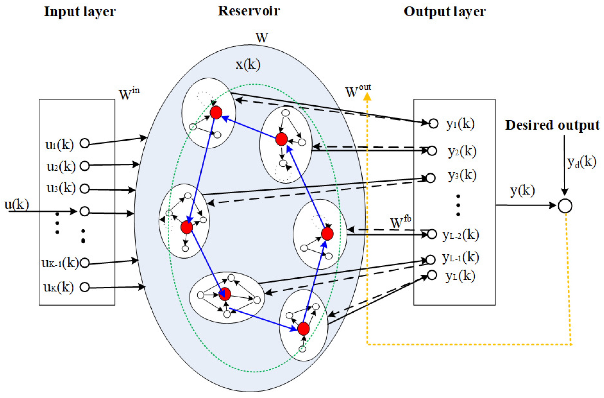
A standard ESN typically consists of an input layer, a reservoir, and an output layer, as shown in Figure 1. The circles in Figure 1 represent neurons.

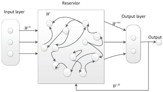
Figure 1. The structure of a standard ESN.

The quantities of input neurons, reservoir neurons, and output neurons are denoted as K, N, and L, respectively. At time step n, the input vector is denoted as $u\left(n\right)={[u_1\left(n\right),u_2\left(n\right),\cdots ,u_K\left(n\right)]}^T$, the state of the reservoir is represented by $x\left(n\right)=[x_1\left(n\right),x_2\left(n\right),$$\cdots ,x_N{\left(n\right)]}^T$, and the output vector is given by $y\left(n\right)=[y_1\left(n\right),y_2\left(n\right),\cdots ,y_L\left(n\right)]$. The given expression can be rewritten as $T^T$. The input weight matrix, denoted as $W^{in}$ with dimensions $N\times K$, represents the weights associated with the input of a system. The reservoir weight matrix, denoted as W with dimensions $N\times N$, represents the weights within the reservoir of the system. The feedback weight matrix, denoted as $W^{fb}$ with dimensions $N\times L$, represents the weights associated with the feedback connections in the system. Lastly, the output weight matrix, denoted as $W^{out}$ with dimensions $L\times (K+N)$, represents the weights associated with the output of the system. Typically, the initial values of $W^{in}$, W, and $W^{fb}$ are predetermined and remain constant during the training of an ESN. Conversely, the weight matrix $W^{out}$ is acquired through the training process of the ESN, representing one of the notable benefits of this approach. The Leaky-ESN is an enhanced variant of the normal ESN, characterized by a reservoir composed of Leaky Integral neurons. The reservoir equation of state proposed by Leaky-ESN is represented as follows [17]:

$$\dot{x}=\frac{1}{c}\left(-ax+f\left(W^{in}u+Wx+W^{fb}y\right)\right),$$

(1)

$$y=g\left(W^{out}\left[x;u\right]\right),$$

(2)

where $c>0$ represents the time constant of the Leaky-ESN model. The parameter $a>0$ corresponds to the leaking rate of the reservoir nodes, which can be interpreted as the rate at which the reservoir state update equation is discretized in time. The function f refers to a sigmoid function used within the reservoir, commonly either the hyperbolic tangent (tanh) or logistic sigmoid function. The function g represents the output activation function, typically either the identity function or the hyperbolic tangent (tanh) function. The notation $\left[;\right]$ denotes the concatenation of two vectors. By employing Euler’s discretization method to the ordinary differential Equation (1) with respect to time, we can accurately derive the discrete equation for the Leaky-ESN model:

$$x\left(n+1\right)=\left(1-a\right)x\left(n\right)+f\left(W^{in}u\left(n+1\right)+Wx\left(n\right)+W^{fb}y\left(n\right)\right),$$

(3)

In Equation (2), the variable $W^{out}$ is both unknown and adjustable, and its computation is necessary throughout the training process of the desired network. During the training phase, the echo states $x\left(n\right)$ are organized into a state collection X in a row-wise manner. Similarly, the learned output values $y\left(n\right)$ that correspond to the $x\left(n\right)$ are arranged in a row-wise vector Y. Next, the calculation of $W^{out}$ is determined using the learning equation in the following manner:

$$W^{out}={\left(X^{T}X\right)}^{-1}{X}^{T}Y,$$

(4)

where $X^T$ represents the transpose of matrix X, while ${\left(X^{T}X\right)}^{-1}$ represents the inverse of the square matrix $\left(X^{T}X\right)$.

The objective of training the ESN is to minimize the error function $E\left(y,d\right)$. The error, denoted as $E\left(y,d\right)$, is commonly represented as a normalized root-mean-square error (NRMSE). The formula for NRMSE is given by

$$E(y,d)=\frac{\sqrt{\frac{1}{n}{\sum }_{i=1}^n{∥y\left(i\right)-d\left(i\right)∥}^2}}{\sigma \left(d\right)},$$

(5)

where $y\left(i\right)$ denotes the ith data of the actual output; $d\left(i\right)$ denotes the ith data of the desired output; $∥·∥$ means the Euclidean distance of a variable; and $\sigma \left(d\right)$ denotes the standard deviation of the desired output.

3. Olfactory Feelings Echo State Network

3.1. The Structure of the OFESN

The subreservoirs of the OFESN may be composed of different types of neurons or the same types of neurons. Here, we assume that the reservoir of the OFESN is composed of m subreservoirs, and each subreservoir is composed of the same types of neurons, i.e., the neuron state update model of each subreservoir is the same. The enrichment of the dynamics of the reservoir can be achieved by constructing an echo state network with the following idea:

(1)

First, m neurons with different initial states are generated, and the Euclidean distance between any two initial states is greater than or equal to a certain number that can be either specified or generated randomly. If this number is randomly generated, the state of neurons of the subreservoirs subsequently generated will be guaranteed to have more complex differences. The m neurons generated above are referred to as master neurons, similar to the master neurons of typical neural circuits, such as olfactory cortex, cerebellar cortex, and hippocampal structures, that are responsible for the input and output of the circuit. Each master neuron becomes the core of each subreservoir and thus becomes the representative of each subreservoir. Let $x_{11}$, $x_{22}$, ⋯$x_{mm}$ denote these m neurons, respectively. Their initial states need to meet the inequality $\left|\right|x_{ii}-x_{jj}\left|\right|\ge {\sigma }_{ij}(i=1,2,\cdots ,m;j=1,2,\cdots ,m)$. Here, ${\sigma }_{ij}$ may be either specified or randomly generated.

(2)

Next, with each master neuron as the center, a subreservoir is constructed around the master neuron. In each subreservoir, the other neurons except the master neuron are called sister neurons. The master neuron and the sister neurons of a subreservoir need to ensure high similarity and correlation. Thus, the master neuron can represent its own subreservoir. The communication between subreservoirs can be realized by the communication between master neurons. The sister neurons belonging to the same subreservoir can communicate with each other, but the sister neurons belonging to a different subreservoir cannot communicate with each other. The m master neurons can construct an m subreservoir, called the actual subreservoir. Let the neurons of the $ith$ subreservoir satisfy $\Vert x_{ii}-x_{ij}\Vert \le {\overline{\sigma }}_{2i}$. Here, $x_{ij}$$(j=1,2,\cdots ,d_i,j\ne i)$ denotes the $jth$ sister neuron of the $ith$ subreservoir, and $d_i$ denotes the number of neurons of the $ith$ subreservoir.

(3)

The OFESN model can provide a new connection mode as follows: (i) The connections between subreservoirs are transformed into the connections between their respective master neurons, which can be determined by the small-world network method or sparse connection. The connections between these master neurons actually generate a virtual and flexible subreservoir. The biggest difference between the virtual reservoir and the actual subreservoir is that the virtual reservoirs are only composed of the master neurons, and thus their neuron states have a bigger difference and less redundant information than those of the actual subreservoir. Therefore, the OFESN is equivalent to having a flexible virtual subreservoir and m actual subreservoirs. (ii) The sister neurons within each subreservoir are sparsely connected. (iii) The sister neurons in different subreservoirs cannot communicate with each other, and there are no connections among them. Such a new connection mode greatly simplifies the coupling connection between neurons in different reservoirs and then reduces the information redundancy. The sparse connection between the master neurons actually creates a virtual subreservoir, which makes the reservoir add a new subreservoir composed of master neurons with large diversity and thus is equivalent to increasing the number of neurons. Therefore, the OFESN model can be more suitable for the situation where the network approximation ability is poor due to the small number of neurons in the whole network reservoir, especially the situation where the number of neurons in each subreservoir is small and the number of subreservoirs is large.

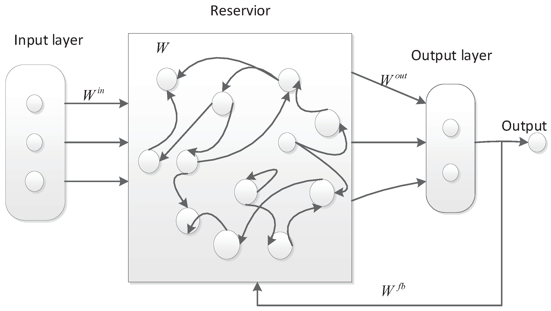
The structure of the OFESN is shown in Figure 2. In Figure 2, the dashed lines from the output layer to the reservoir represent $W^{fb}$,  the solid lines from the reservoir to the output layer represent $W^{out}$, and the colored dotted line means that $W^{out}$ can be adjusted online such that the network output $y\left(k\right)$ follows $y_d\left(k\right)$, in addition to being calculated by Equation (4). The ellipses of the black line in the reservoir represent actual subreservoirs, respectively. In each subreservoir, a circle filled with red denotes its master neuron. All master neurons construct a virtual subreservoir denoted by the ellipses of the green dotted line. The neurons of each actual subreservoir, including its master neuron and the sister neurons, use the sparse connection. Each subreservoir can be represented by its master neuron, and then the connections between actual subreservoirs can be determined by the connections between master neurons. The master neurons, i.e., the neurons of the virtual subreservoir, may use sparse connection or the small-world network method.

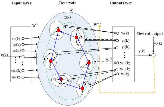
Figure 2. The structure of the OFESN.

The state update equation of the OFESN is as follows:

$$x\left(n+1\right)=\left(1-a\right)x\left(n\right)+f\left(W^{in}u\left(n+1\right)+Wx\left(n\right)+W^{fb}y\left(n\right)\right),$$

(6)

$$y\left(n\right)=g\left(W^{out}\left[x\left(n\right);u\left(n\right)\right]\right),$$

(7)

where $x\left(n\right)={[x_1^T\left(n\right),x_2^T\left(n\right),\cdots ,x_m^T\left(n\right)]}^T$ denotes the state vector of the reservoir and $x_i\left(n\right)={[x_{i1},x_{i2},\cdots ,x_{i{d}_i}]}^T$ denotes the state of the subreservoir. $d_i$ indicates the number of neurons of the ith subreservoir. $W^{in}$, W, $W^{fb}$ are the input connection weight matrix, the reservoir neuron connection weight matrix, and the output feedback connection weight matrix, respectively. The reservoir neuron connection weight matrix takes the following form:

$$\begin{array}{c}\hfill W=\left[\begin{array}{cccc}{W}_1& W_{12}& \cdots & W_{1m}\\ W_{21}& W_{22}& \cdots & W_{2m}\\ ⋮& ⋮& \ddots & ⋮\\ W_{m1}& W_{m2}& \cdots & W_m\end{array}\right]\end{array}$$

where $W_{ij}$ is the connection weight matrix between the ith subreservoir and the jth subreservoir, $W_1$, $W_2$, ⋯, $W_m$ denote the internal connection weight matrix of m actual subreservoirs, which can be generated randomly with a certain sparsity. The dimensions of W, $W_{ij}$, and $W_i$ are ${\displaystyle \sum _{i=1}^m}{d}_i\times {\displaystyle \sum _{i=1}^m}{d}_i$, $d_i\times d_j$, and $d_i\times d_i$, respectively.

The following is an example of how to generate $W_{12}$, $W_{13}$, ⋯, $W_{1m}$ to explain how to generate $W_{ij}$. $W_{12}$ denotes the connection weight matrix between the 1st subreservoir and the 2nd subreservoir. To reduce information redundancy and simplify the connections between neurons, the OFESN uses the connections between the master neuron of the 1st subreservoir and the master neuron of the 2nd subreservoir to represent the connections between the 1st subreservoir and the 2nd subreservoir. We assume that the first neuron of the first subreservoir is the principal neuron and the second neuron of the second subreservoir is the master neuron. Thus, the element in the 1st row and the 2nd column of $W_{12}$ denotes the connection weights between the master neuron of the 1st subreservoir and the master neuron of the 2nd subreservoir, which can be expressed as ${\overline{W}}_{12}$. ${\overline{W}}_{12}$ may be a zero or nonzero value. ${\overline{W}}_{12}=0$ represents that there is no connection between the master neuron of the 1st subreservoir and the master neuron of the 2nd subreservoir. ${\overline{W}}_{12}\ne 0$ represents that there is a connection between the master neuron of the 1st subreservoir and the master neuron of the 2nd subreservoir. In other words, only ${\overline{W}}_{12}$ of $W_{12}$ may be a nonzero element, and the rest of the elements $W_{12}$ are zero. Similarly, the element in the 1st row and 3rd column of $W_{13}$, denoted by ${\overline{W}}_{13}$, represents the connection weights between the master neuron of the 1st subreservoir and the master neuron of the 3rd subreservoir. Only the ${\overline{W}}_{13}$ of $W_{13}$ may be a nonzero element, and the rest of the elements $W_{13}$ are zero. So, the element in the 1st row and mth column of $W_{1m}$ is denoted by ${\overline{W}}_{1m}$. Only the ${\overline{W}}_{1m}$ of $W_{1m}$ may be a nonzero element, and the rest of the elements $W_{1m}$ are zero. The values of ${\overline{W}}_{12}$, ${\overline{W}}_{13}$, ⋯, ${\overline{W}}_{1m}$ are determined by the connection weights between the neurons of the virtual subreservoir, and ${\overline{W}}_{12}$, ${\overline{W}}_{13}$, ⋯, ${\overline{W}}_{1m}$ is actually the corresponding element of the connection weight matrix $\overline{W}$ of the virtual subreservoir.

From the above, the element in the ith row and the jth column of $W_{ij}$, denoted by ${\overline{W}}_{ij}$, represents the connection weights between the master neuron of the ith subreservoir and the master neuron of the jth subreservoir. Only one element of $W_{ij}$ is possibly nonzero, and the rest of the elements of $W_{ij}$ are zero. The possibly nonzero element characterizes the master neuron of the ith subreservoir possibly connected with the master neuron of the jth subreservoir, and its value is determined by the random sparse connection of the virtual subreservoir. ${\overline{W}}_{ii}$ represents the connection of the master neuron itself in the ith subreservoir. So, $\overline{W}$ is made up of ${\overline{W}}_{ij}$$(i=1,2,\cdots ,m,j=1,2,\cdots ,m)$. Let ${\overline{W}}_{ii}=0$, which is the equivalent of ${\overline{W}}_{ii}$ added to $W_i$. $\overline{W}$ can be generated randomly with a spectral radius less than 1 and a certain sparsity. It is especially worth noting that the connection weight matrix of reservoir W is asymmetric; that is, the connection between reservoir neurons is duplex.

In addition, in Equation (7), the input matrix $W^{in}$ and feedback connection weight matrix $W^{fb}$ are in the following form:

$$\begin{array}{c}\hfill W^{in}=\left[\begin{array}{cccc}{\left(W_1^{in}\right)}^T& {\left(W_2^{in}\right)}^T& \cdots & {\left(W_m^{in}\right)}^T\end{array}\right]\end{array}$$

$$\begin{array}{c}\hfill W^{fb}=\left[\begin{array}{cccc}{\left(W_1^{fb}\right)}^T& {\left(W_2^{fb}\right)}^T& \cdots & {\left(W_m^{fb}\right)}^T\end{array}\right]\end{array}$$

After the matrix is normalized, Equation (6) is rewritten as

$$x\left(n+1\right)=\left(1-a\right)x\left(n\right)+f\left(S^{in}{W}^{in}u\left(n+1\right)+\rho Wx\left(n\right)+S^{fb}{W}^{fb}y\left(n\right)\right),$$

(8)

where $S^{in}$ is the input scaling factor, $\rho$ is the spectral radius, and $S^{fb}$ is the output feedback scaling factor.

After normalization, W, $W^{in}$, $W^{fb}$ can be, respectively, rewritten as

$$\begin{array}{c}\hfill W=\left[\begin{array}{cccc}{\rho }_1{W}_1& W_{12}& \cdots & W_{1m}\\ W_{21}& {\rho }_2{W}_{22}& \cdots & W_{2m}\\ ⋮& ⋮& \ddots & ⋮\\ W_{m1}& W_{m2}& \cdots & {\rho }_3{W}_m\end{array}\right]\end{array}$$

$$\begin{array}{c}\hfill W^{in}=\left[\begin{array}{cccc}{\left(S_1^{in}{W}_1^{in}\right)}^T& S_2^{in}{\left(W_2^{in}\right)}^T& \cdots & S_m^{in}{\left(W_m^{in}\right)}^T\end{array}\right]\end{array}$$

$$\begin{array}{c}\hfill W^{fb}=\left[\begin{array}{cccc}{\left(S_1^{fb}{W}_1^{fb}\right)}^T& S_2^{fb}{\left(W_2^{fb}\right)}^T& \cdots & S_m^{fb}{\left(W_m^{fb}\right)}^T\end{array}\right]\end{array}$$

among them, $W_i$, $W_i^{in}$, $W_i^{fb}$ is the normalized matrix.

3.2. The Echo State Property of the OFESN

Theorem 1 ([28]).

For a discrete OFESN model (8), if the following conditions are satisfied:

(i) 

f selects sigmoid function (tanh);

(ii) 

The output activation function g is a bounded function (for example, tanh) or $W^{fb}=0$;

(iii) 

There are no output feedbacks, that is, $W^{fb}=0$;

(iv) 

$|1-a+\rho {\delta }_{max}| <1$ (where ${\delta }_{max}$ is the maximal singular value of W);

the OFESN model has the echo state property.

In order to ensure that the OFESN satisfies the echo state property, the reservoir connection weight matrix must satisfy Theorem 1. In fact, each subreservoir does not need to meet the echo state property, as long as the entire reservoir does.

Proof. 

For any two states $x\left(n+1\right)$ and $x^{\prime }\left(n+1\right)$ of the reservoir at time $n+1$ [23], the following holds:

$$\begin{array}{ccc}\hfill & & ∥x(n+1)-x^{\prime }(n+1)∥\hfill \\ & =& ∥(1-a)(x\left(n\right)-x^{\prime }\left(n\right))+(f(S^{in}{W}^{in}u\left(n+1\right)+\rho Wx\left(n\right))-f(S^{in}{W}^{in}u\left(n+1\right)+\rho W{x}^{\prime }\left(n\right))∥\hfill \\ & \le & (1-a)∥x\left(n\right)-x^{\prime }\left(n\right)∥+∥f(S^{in}{W}^{in}u\left(n+1\right)+\rho Wx\left(n\right))-f(S^{in}{W}^{in}u\left(n+1\right)+\rho W{x}^{\prime }\left(n\right))∥\hfill \\ & \le & (1-a)∥x\left(n\right)-x^{\prime }\left(n\right)∥+\rho ∥Wx\left(n\right)-W{x}^{\prime }\left(n\right)∥\hfill \\ & \le & (1-a+\rho {\delta }_{max})∥x\left(n\right)-x^{\prime }\left(n\right)∥\hfill \end{array}$$

(9)

Thus, $|1-a+\rho {\delta }_{max}|$ is a global Lipschitz rate by which any two states approach each other in the state update. To guarantee that the OFESN has the echo state property, the inequality (10) must be satisfied.

$$\begin{array}{c}\hfill |1-a+\rho {\delta }_{max}|<1,\end{array}$$

(10)

hence, the proof is complete.    □

3.3. Optimizing the Global Parameters of OFESN

The models to be optimized here are Equations (7) and (8). The parameters to be optimized are a, $S_i^{in}$, $S_i^{fb}$, ${\rho }_i$, $\overline{\rho }$ (spectral radius of matrix), and $W^{out}$. $W^{out}$ can be solved by linear regression method, such as pseudoinverse method. In order to simplify the operation, ${\rho }_i$, ${\sigma }_{ij}$, ${\overline{\sigma }}_{2i}$ is not optimized and is given in advance. Only the $q\in \{a,S_i^{in},S_i^{fb},\overline{\rho }\}$ parameters are optimized, and echo state property conditions are satisfied. In this paper, stochastic gradient descent method is used to optimize these parameters. Here, $i=1,2,\cdots ,m$.

When $W^{fb}=0$, invoke the chain rule and observe (8); we obtain $\frac{\partial x\left(n\right)}{\partial q}$:

$$\begin{array}{c}\hfill \frac{\partial x\left(n\right)}{\partial a}=(1-a)\frac{\partial x\left(n-1\right)}{\partial a}-x\left(n-1\right)+f^{\prime }\left(x\right).\ast (\overline{\rho }W\frac{\partial x\left(n-1\right)}{\partial a}),\end{array}$$

(11)

$$\begin{array}{c}\hfill \frac{\partial x\left(n\right)}{\partial \overline{\rho }}=(1-a)\frac{\partial x\left(n-1\right)}{\partial \overline{\rho }}+f^{\prime }\left(x\right).\ast (\overline{\rho }W\frac{\partial x\left(n-1\right)}{\partial \overline{\rho }}+Wx(n-1)),\end{array}$$

(12)

$$\begin{array}{c}\hfill \frac{\partial x\left(n\right)}{\partial S_i^{in}}=(1-a)\frac{\partial x\left(n-1\right)}{\partial S_i^{in}}+f^{\prime }\left(x\right).\ast (\overline{\rho }W\frac{\partial x\left(n-1\right)}{\partial S_i^{in}}+\frac{\partial W^{in}}{\partial S_i^{in}}u\left(n\right)),\end{array}$$

(13)

$$\begin{array}{c}\hfill \frac{\partial x\left(n\right)}{\partial S_i^{fb}}=(1-a)\frac{\partial x\left(n-1\right)}{\partial S_i^{fb}}+f^{\prime }\left(x\right).\ast (\overline{\rho }W\frac{\partial x\left(n-1\right)}{\partial S_i^{fb}}),\end{array}$$

(14)

where $.\ast$ denotes the element-wise product of two vectors.

When containing $W^{fb}$, let $X\left(n\right)=S^{in}{W}^{in}u\left(n+1\right)+\rho Wx\left(n\right)+S^{fb}{W}^{fb}y\left(n\right)$. Here, we use a simple symbol $0_u={\left(0,\cdots ,0\right)}^T$ to represent the input vector whose entries are all zeros; the $\frac{\partial y\left(n\right)}{\partial q}=W^{out}[\frac{\partial x\left(n-2\right)}{\partial q};0_u]$, and we obtain $\frac{\partial x\left(n\right)}{\partial q}$:

$$\begin{array}{c}\hfill \frac{\partial x\left(n\right)}{\partial a}=(1-a)\frac{\partial x\left(n-1\right)}{\partial a}-x\left(n-1\right)+f^{\prime }\left(x\right).\ast (\overline{\rho }W\frac{\partial x\left(n-1\right)}{\partial a}+W^{fb}{W}^{out}[\frac{\partial x\left(n-2\right)}{\partial a};0_u]),\end{array}$$

(15)

$$\begin{array}{c}\hfill \frac{\partial x\left(n\right)}{\partial \overline{\rho }}=(1-a)\frac{\partial x\left(n-1\right)}{\partial \overline{\rho }}+f^{\prime }\left(x\right).\ast (\overline{\rho }W\frac{\partial x\left(n-1\right)}{\partial \overline{\rho }}+Wx(n-1)+W^{fb}{W}^{out}[\frac{\partial x\left(n-2\right)}{\partial \overline{\rho }};0_u]),\end{array}$$

(16)

$$\begin{array}{c}\hfill \frac{\partial x\left(n\right)}{\partial S_i^{in}}=(1-a)\frac{\partial x\left(n-1\right)}{\partial S_i^{in}}+f^{\prime }\left(x\right).\ast (\overline{\rho }W\frac{\partial x\left(n-1\right)}{\partial S_i^{in}}+\frac{\partial W^{in}}{\partial S_i^{in}}u\left(n\right)+W^{fb}{W}^{out}[\frac{\partial x\left(n-2\right)}{\partial S_i^{in}};0_u]),\end{array}$$

(17)

$$\begin{array}{c}\hfill \frac{\partial x\left(n\right)}{\partial S_i^{fb}}=(1-a)\frac{\partial x\left(n-1\right)}{\partial S_i^{fb}}+f^{\prime }\left(x\right).\ast (\overline{\rho }W\frac{\partial x\left(n-1\right)}{\partial S_i^{fb}}+\frac{\partial W^{fb}}{\partial S_i^{fb}}y\left(n\right)+W^{fb}{W}^{out}[\frac{\partial x\left(n-2\right)}{\partial S_i^{fb}};0_u]),\end{array}$$

(18)

In other words, to train the output weight matrix $W_{out}$, the output $y\left(n\right)$ should be as close as possible to the teacher output $d\left(n\right)$ during the training process. The error $\epsilon \left(n\right)$ expression is as follows:

$$\begin{array}{c}\hfill \epsilon \left(n\right)=y\left(n\right)-d\left(n\right),\end{array}$$

(19)

we define the squared error $E\left(n\right)$ as follows:

$$\begin{array}{c}\hfill E\left(n\right)=\frac{1}{2}{∥\epsilon \left(n\right)∥}^2,\end{array}$$

(20)

to $0_u={\left(0,\cdots ,0\right)}^T$, there is

$$\begin{array}{c}\hfill \frac{\partial E\left(n+1\right)}{\partial q}=-\epsilon \left(n+1\right)W^{out}[\frac{\partial x\left(n-1\right)}{\partial q};0_u],\end{array}$$

(21)

the global parameter update expression is as follows:

$$\begin{array}{c}\hfill q\left(n+1\right)=q\left(n\right)-K\frac{\partial E\left(n+1\right)}{\partial q},\end{array}$$

(22)

K represents the learning rate of the global parameter q. The parameters modified in this process must ensure that the OFESN model has the echo state property in practical applications.

3.4. Implementation of the OFESN

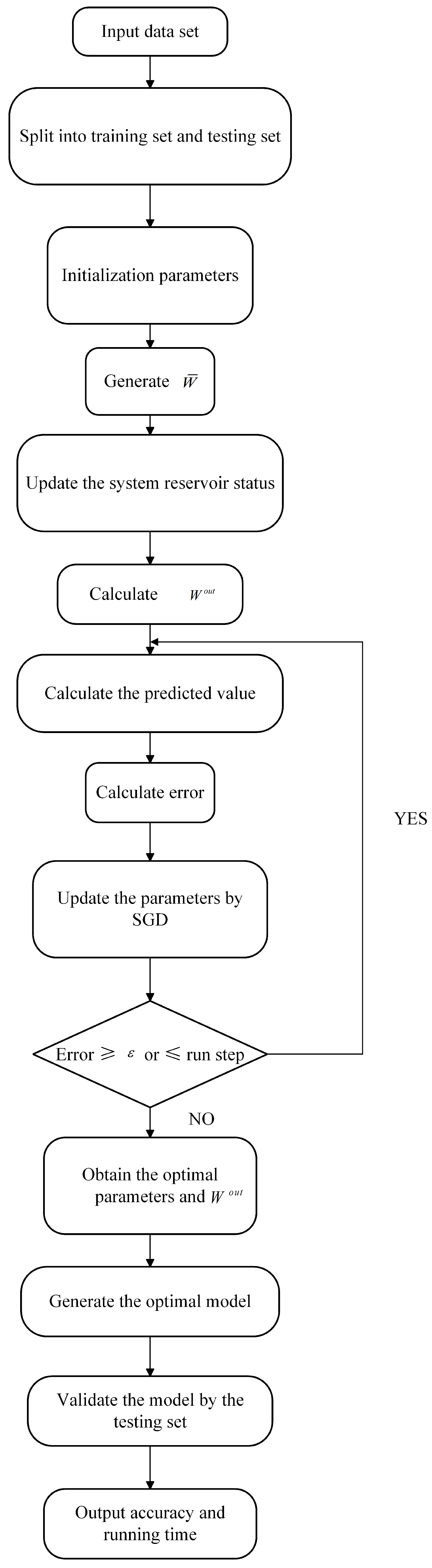
The simulation flow chart is shown in Figure 3, and the steps for OFESN implementation are as follows:

Figure 3. OFESN test error at different initial value and different connection.

(i)

Assume that the reservoir of the OFESN is composed of m classes of neurons, and each class of neurons constitutes a subreservoir, and the number of neurons in the ith reservoir is $d_i$, then the total number of neurons in the reservoir is $N={\displaystyle \sum _{i=1}^m}{d}_i$.

(ii)

Initialize the parameters, including the sparse degree, run step, learning rate, and connection weight matrix $W^{in}$ and $W^{fb}$, as well as the parameters to be optimized a, $\rho$, $S_i^{in}$, $S_i^{fb}$.

(iii)

The master neurons of m subreservoir constitute a virtual subreservoir, and its corresponding connection weight is $\overline{W}$ that is randomly generated and has a certain sparsity.

(iv)

Initialization of m master neurons. Let $x_{11},x_{22},x_{33},\cdots ,x_{mm}$ (m) be given, respectively, and let their initial state satisfy $|x_{ii}-x_{jj}|\ge {\sigma }_{ij}$, and ${\sigma }_{ij}$ can be either specified or randomly generated.

(v)

The other sister neurons of m subreservoirs generate initial states. With master neuron $x_{ii}(i=1,2,\cdots ,m)$ as the center, multiple sister neurons with high similarity and high correlation are formed into the ith subreservoir, and the neuron state of the ith subreservoir meets $|x_{ii}-x_{ij}|\le {\overline{\sigma }}_{2i}$.

(vi)

The internal connection weight matrix $W_i$$(i=1,2,\cdots ,m)$ of the ith actual subreservoir can be randomly generated, has certain sparsity, and may satisfy the spectral radius of less than 1. $\overline{W}$ is composed of ${\overline{W}}_{ij}$, among which $(i=1,2,\cdots ,m,j=1,2,\cdots ,m)$ can be randomly generated with a spectral radius less than 1 and a certain sparsity. The spectral radius of $W_i$ and ${\overline{W}}_{ij}$ may not be less than 1, but the echo state property condition must be satisfied as inequality (10).

(vii)

Update the system reservoir states according to (8).

(viii)

The optimal parameters and $W^{out}$ were obtained at the end of the training.

(ix)

Test OFESN accuracy and running time.

The implementation pseudocode is shown in Algorithm 1:

Algorithm 1: OFESN algorithm
	Input: Dataset, number of reservoirs m, number of ith reservoir $d_i$, sparse degree, run step, learning rate K, ${\sigma }_{ij}$, $\overline{{\sigma }_{2j}}$
	Output: Testing set accuracy and running time
1	Split the dataset into a training set and a testing set;
2	Initialize parameters: $W^{in}$, $W^{fb}$, $a,\rho ,S_i^{in},S_i^{fb}$
3	$\overline{W}$← master neurons:$\left|x_{ii}-x_{jj}\right|\ge {\sigma }_{ij}$, subreservoir:$\left|x_{ii}-x_{ij}\right|\le \overline{{\sigma }_{2j}}$
4	while error ≥$\epsilon$ or n≤ run step do
5	Update the system reservoir states according to Equation (8);
6	Calculate $W^{out}$ according to Equation (4);
7	Calculate the predicted value according to Equation (7);
8	Calculate error;
9	Update the parameters by SGD;
10	$n\leftarrow n+1$;
11	end
12	Return $a,\rho ,S_i^{in},S_i^{fb}$, $W^{out}$;
13	Generate the optimal model;
14	Validate accuracy by the testing set;

4. Verification by Experiment Simulation

To verify the effectiveness of the OFESN, sine superposition function and Mackey–Glass were used, and comparisons between the OFESN with Leaky-ESN are given in terms of run time and prediction accuracy.

4.1. Simulation Example 1

In this section, a sine superposition function is given as follow:

$$\begin{array}{c}\hfill u_1\left(n\right)=sin\left(n\right)+sin\left(0.51n\right)+sin\left(0.22n\right)+sin\left(0.1002n\right)+sin\left(0.05343n\right),\end{array}$$

(23)

The teacher output $d_1\left(n\right)$ is

$$\begin{array}{c}\hfill d_1\left(n\right)=u_1\left(n-5\right),\end{array}$$

(24)

According to Equations (23) and (24), we generate 20,500 data samples, which are divided into three parts: 20,000 training samples (100 initial washout samples) and 500 testing samples. The sample point, or epoch, is set at 500 times, and a total of 20,000 times results in 40 points. In this context, it is necessary to examine two scenarios pertaining to the size of the reservoir. The first group consists of 36 neurons, while the second group consists of 17 neurons. When the size of the reservoir, denoted as N, is equal to 36, the reservoir can be categorized into two categories based on the number of subreservoirs it contains, i.e., the reservoir with either 6 subreservoirs or 3 subreservoirs. In each case, the model performs 20 times in a random manner. The resulting mean and standard deviation of the NRNSE are then gathered. Subsequently, error bar graphs are constructed to visually represent these values.

4.1.1. The Structure of 3 Actual Subreservoirs

The reservoir contains 3 actual subreservoirs, the number of neurons in the ith actual subreservoir is denoted by $N_i$ (i = 1, 2, 3). Here, the number of neurons in the virtual subreservoir is denoted by $N_4$. Assuming that the actual subreservoirs are $N_i=12$ and the virtual subreservoir is $N_4=3$, different initial values were selected for parameter a, $\overline{\rho }$, $S_i^{in}$, and the different sparsity of neuron connections in the subreservoir was tested. In this section, a, $\overline{\rho }$, $S_i^{in}$ take two different initial values. The first case is $[a\left(0\right),\overline{\rho }\left(0\right),S_i^{in}\left(0\right)]=[1;0.5\ast rand\left(1\right);0.15\ast rand\left(1\right)]$, and the second case is $[a\left(0\right),\overline{\rho }\left(0\right),S_i^{in}\left(0\right)]=[0.8;0.6;0.1]$. Here, $rand\left(1\right)$ denotes a random number uniformly distributed within the interval $(0,1)$. Then, the connections between neurons in each subreservoir can be divided into two cases of fully connections and partially connections. In view of different initial values of the parameters and the different connections between neurons in each subreservoir, simulation tests are carried out in this section. The results are shown in Figure 1, Figure 2, Figure 3, Figure 4, Figure 5, Figure 6, Figure 7, Figure 8 and Figure 9, respectively. The figure is an error bar diagram of NRMSE. Error bars are calculated using mean and standard deviation. The standard deviation is obtained by dividing by M − 1, where M represents the number of samples.

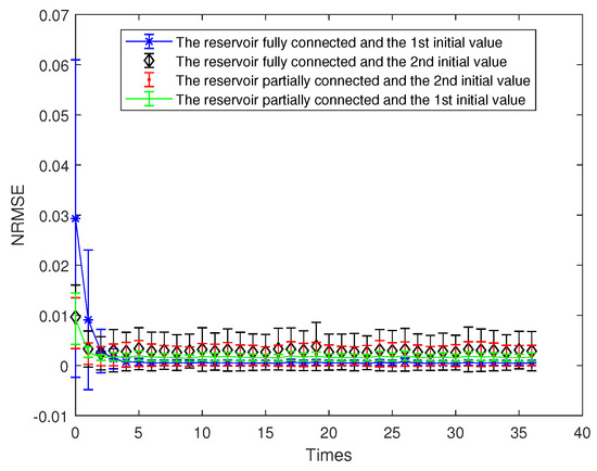
Figure 4. OFESN test error at different initial value and different connection.

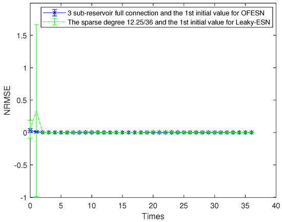
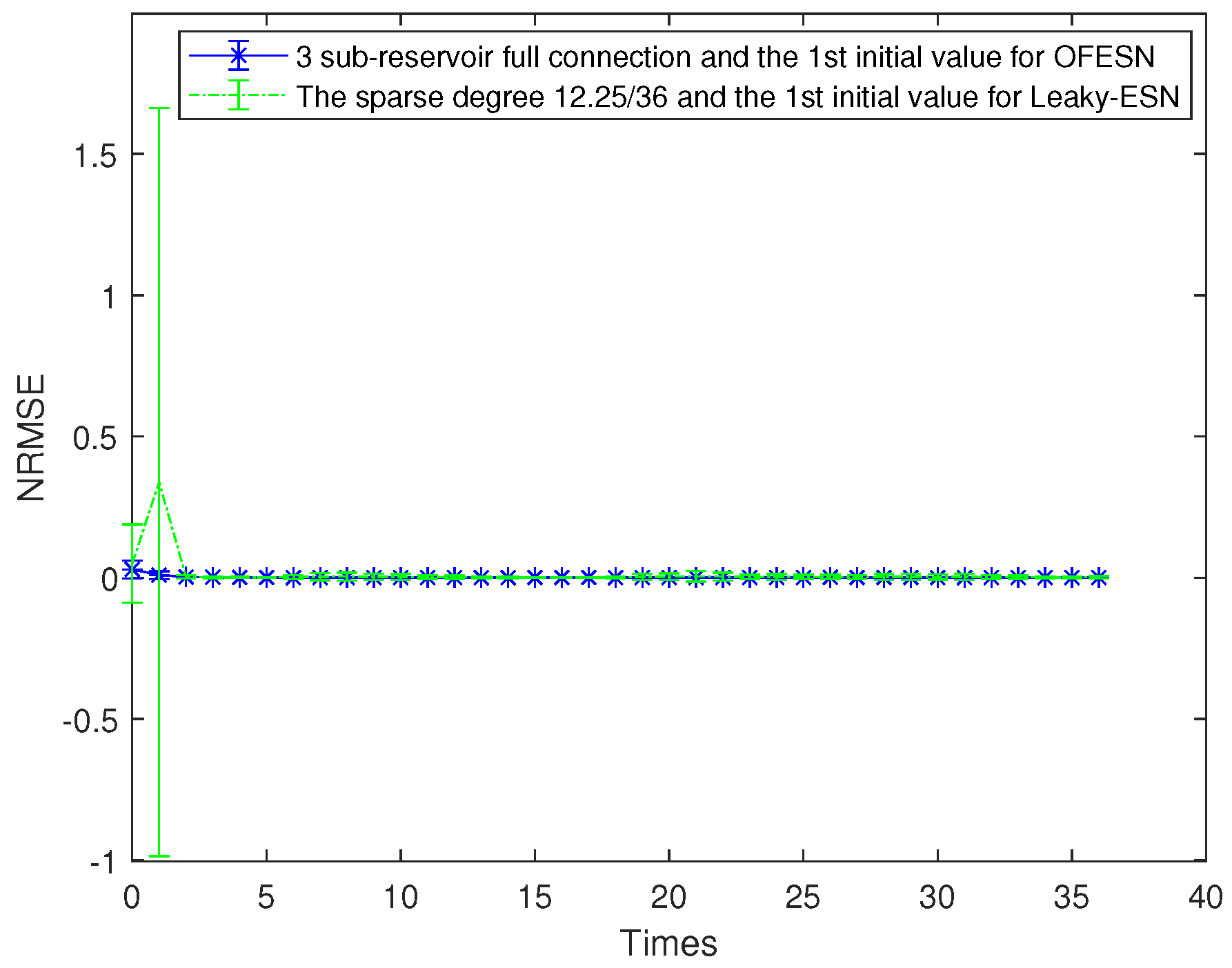
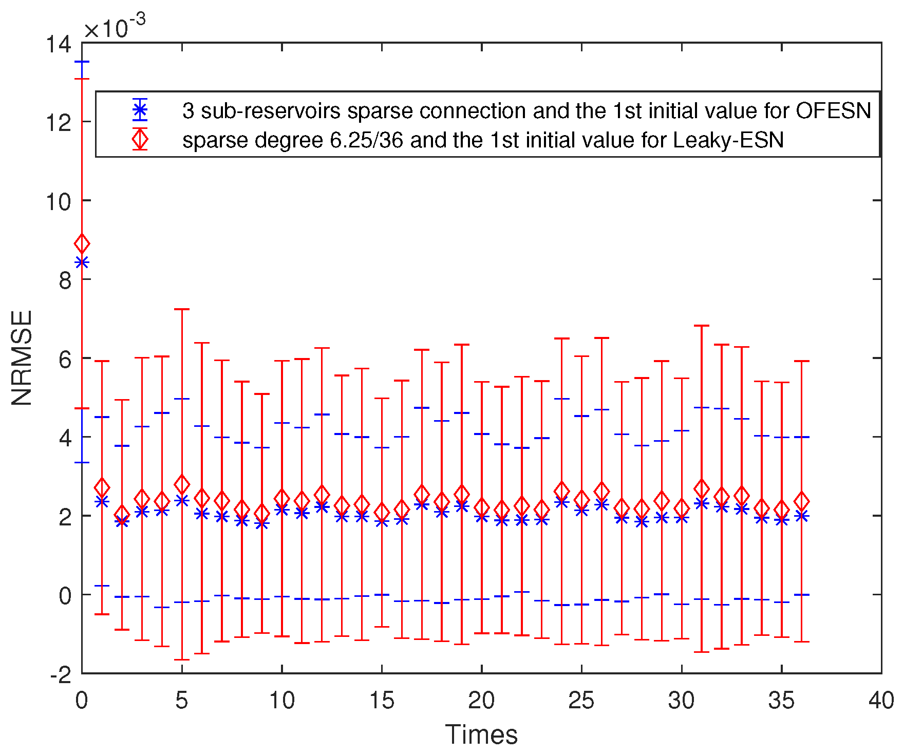
Figure 5. Comparison between the OFESN with full connection and Leaky-ESN with a sparse degree of $\frac{12.25}{36}$ at the first initial value.

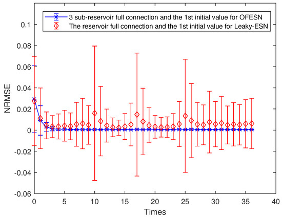
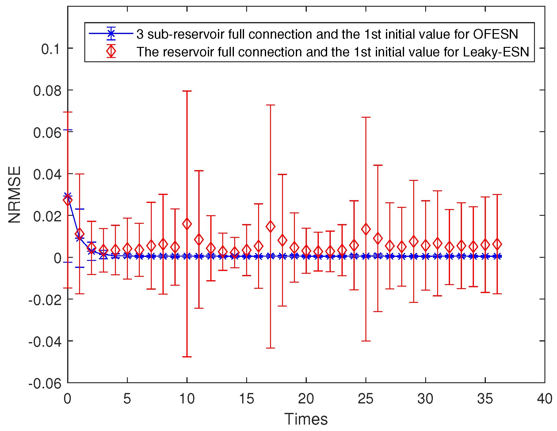
Figure 6. Comparison between the OFESN with subreservoirs fully connected and Leaky-ESN with full connection at the first initial value.

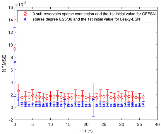
Figure 7. Comparison between the OFESN and Leaky-ESN at the partially connected reservoir and the first initial value.

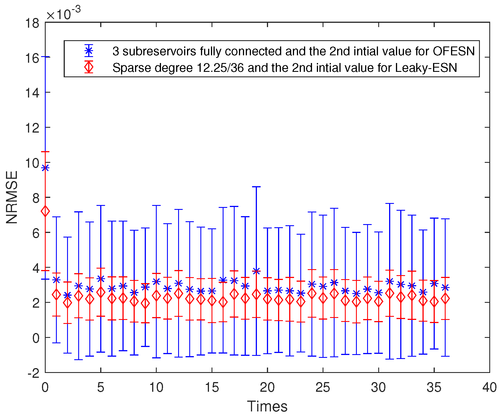
Figure 8. Comparison between the OFESN with fully connected subreservoir and Leaky-ESN with the sparse degree of $\frac{12.25}{36}$ at the second initial value.

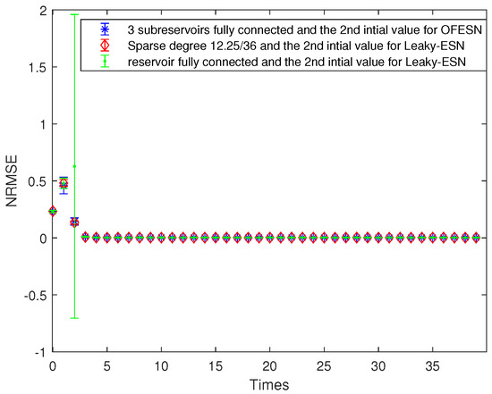
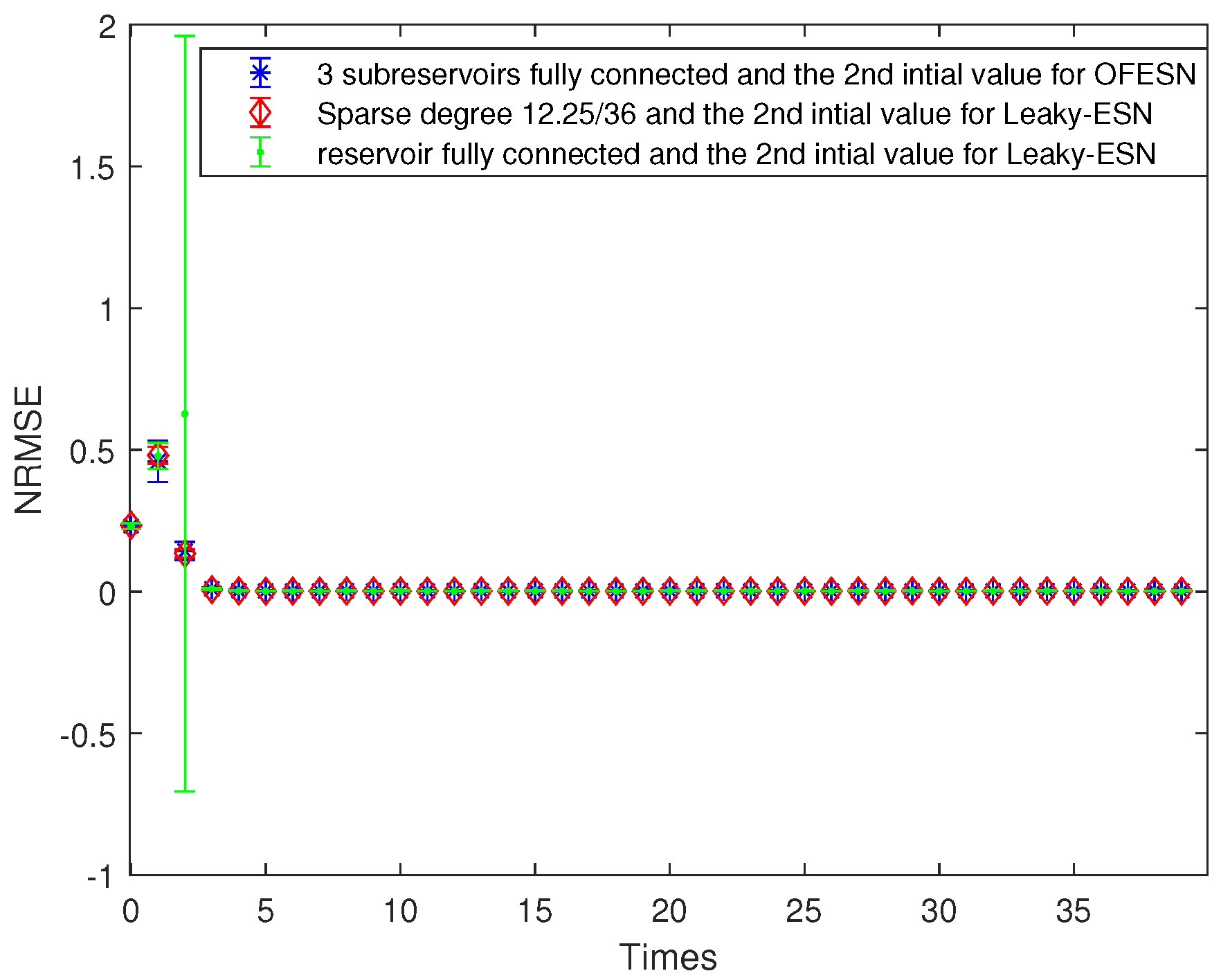
Figure 9. Comparison of Leaky-ESN with fully connected reservoir and the OFESN with all subreservoirs fully connected.

In the initial phase of network model, the prediction error is slightly larger. In order to see the details of subsequent prediction errors, the initial 3 prediction error points are usually not drawn in the figure; so, there are only 37 data points. In addition, usually $x\left(n\right)$ data from the beginning of the training run are discarded (i.e., not used for learning $W^{out}$) since they are contaminated by initial transients. Figure 4 shows the prediction error diagram of the OFESN proposed in this paper when parameters are different initial values and the subreservoir is fully connected or partially connected.

(i).

The first initial value case and the subreservoir fully connected (called Case 1)

$[a\left(0\right),\overline{\rho }\left(0\right),S_i^{in}\left(0\right)]=[1;0.5\ast rand\left(1\right);0.15\ast rand\left(1\right)]$. The internal neurons of each subreservoir are fully connected, i.e., the sparse degree of each actual subreservoir is 1, and the sparse degree of the virtual subreservoir is also 1. Thus, the number of the nonzero internal connection weights in the whole reservoir $N_{c\_Full}$ is approximately calculated as follows:

$$\begin{array}{c}\hfill N_{c\_Full\_3}=\sum _{i=1}^3{N}_i\ast N_i+N_4\ast N_4\end{array}$$

(25)

According to Equation (25), $N_{c\_Full\_3}=441$. To make Leaky-ESN have the same number of nonzero internal connection weights, its corresponding sparse degree should be calculated as follows:

$$\begin{array}{c}\hfill N_{c\_Full\_3}=N\ast N\ast \frac{S_1}{N}\end{array}$$

(26)

where $\frac{S_1}{N}$ represents the sparse degree of the reservoir. According to Equation (26) and $N=36$, $S_1=12.25$ is obtained, and then Leaky-ESN has a sparse degree of $\frac{12.25}{N}$. Figure 5 shows the prediction accuracy comparison between the OFESN and Leaky-ESN. In Figure 6, the performance of Leaky-ESN with a fully connected reservoir is given.

As can be seen from Figure 5 and Figure 6, the OFESN has higher error accuracy in the training process, and the error fluctuation range is smaller than Leaky-ESN, which verifies the effectiveness of the OFESN model.

(ii).

The firs initial value case and the partially connected subreservoir (called Case 2)

The sparse degree of the 3 subreservoirs of the OFESN is selected as $\frac{6}{N_i}(i=1,2,3)$, respectively, and the virtual subreservoir composed of 3 master neurons uses full connection. Then, the number of internal connection weights in the whole reservoir is calculated as follows:

$$\begin{array}{c}\hfill N_{c\_partial\_3}=\sum _{i=1}^3{N}_i\ast N_i\ast \frac{6}{N_i}+N_4\ast N_4\end{array}$$

(27)

According to Equation (27), $N_{c\_partial\_3}=225$. The Leaky-ESN with the same number of internal connection weights should have a sparse degree of reservoir as follows:

$$\begin{array}{c}\hfill N_{c\_partial\_3}=N\ast N\ast \frac{S_2}{N}\end{array}$$

(28)

Solve Equation (28) and obtain $S_2=6.25$. Thus, the sparse degree of the corresponding leaky-ESN should be set to $\frac{6.25}{36}$, which is consistent with the number of neurons interconnections in the reservoir of the OFESN. Here, the neuron interconnections include the self-connection of neurons, the two-way connection between two neurons, and one-way connection between two neurons.

Figure 7 shows the comparison of prediction error bars between the OFESN and Leaky-ESN. It can be seen that in the training process, the OFESN is superior to Leaky-ESN in terms of error accuracy and error stability, which further verifies the effectiveness of the OFESN model.

(iii).

The second initial value case and the fully connected subreservoir (called Case 3)

The initial value is the second case; that is, $[a\left(0\right),\overline{\rho }\left(0\right),S_i^{in}\left(0\right)]=[0.8;0.6;0.1]$, and the sparse degree of the 3 actual subreservoirs is 1, and the sparse degree of the virtual subreservoir is also 1. Similar to Equations (25) and (26), the corresponding sparse degree of Leaky-ESN should be set to $\frac{12.25}{36}$, which is the same as the number of neuron interconnections in the OFESN reservoir.

Figure 8 shows the prediction accuracy comparison between the OFESN and Leaky-ESN. Figure 9 shows the performance of Leaky-ESN with fully connected reservoir and the performance of the OFESN with all subreservoirs fully connected. As can be seen from Figure 8 and Figure 9, the prediction performance of the OFESN is better than Leaky-ESN, and the prediction error fluctuation is also much smaller than Leaky-ESN.

(iv).

The second initial value case and the partially connected subreservoir (called Case 4)

The sparse degree of the 3 actual subreservoirs is $\frac{6}{N_i}(i=1,2,3)$, respectively. The virtual subreservoir composed of the 3 master neurons is fully connection, and its sparse degree is 1. Similar to Equations (27) and (28), the corresponding sparse degree of Leaky-ESN should be set to $\frac{5.8}{36}$. This makes leaky-ESN have the same number of nonzero internal connection weights as the OFESN. The comparison of train accuracy of the two models is shown in Figure 10. It can be seen that in the whole training process, the OFESN partially connected to the reservoir has better prediction performance than Leaky-ESN.

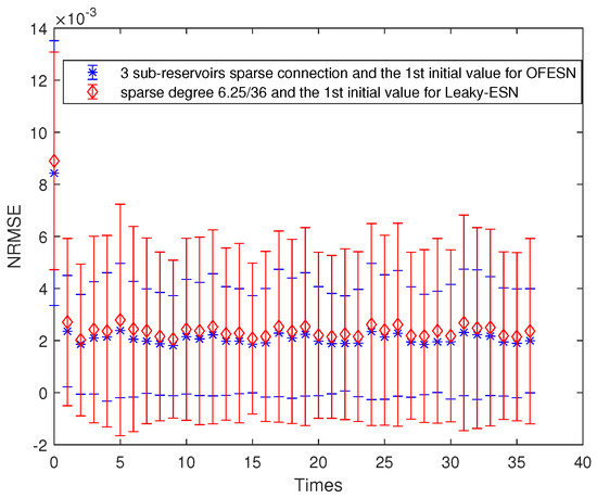
Figure 10. Comparison between the OFESN and Leaky-ESN at the partially connected reservoir and the second initial value.

4.1.2. The Structure of Six Actual Subreservoirs

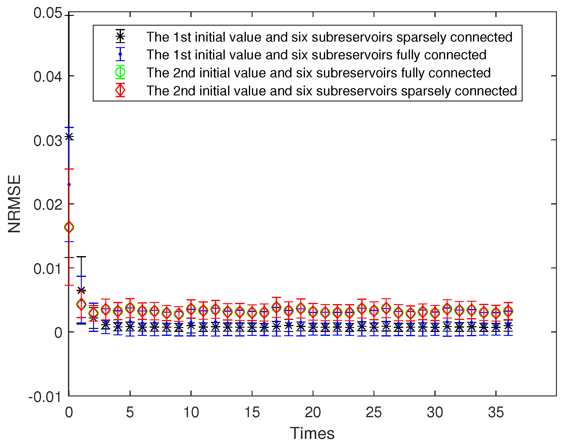
The OFESN reservoir is divided into 6 actual subreservoirs, and the number of neurons in the ith actual subreservoir is denoted by $N_i$$(i=1,2,\cdots ,6)$. Thus, the number of neurons in the virtual subreservoir, denoted by $N_7$, is $N_7=6$. The prediction accuracy of the OFESN and Leaky-ESN is compared for the two different initial values of parameters a, $\overline{\rho }$, and $S_i^{in}$, respectively, and the two kinds of connections, including partial connection and full connection of the subreservoirs. Figure 11 shows the prediction accuracy of the OFESN under different conditions. It can be seen that under the condition of sparsely connected and fully connected, the OFESN is convergent, and the error is stable between 0 and 0.005.

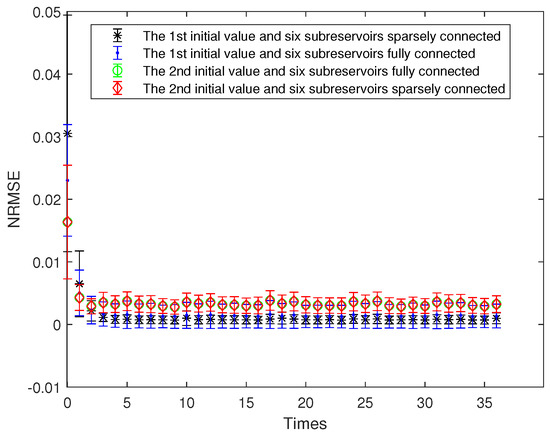
Figure 11. Prediction error bars of the OFESN under different conditions.

(i).

The first initial value case and the fully connected subreservoir (called Case 1)

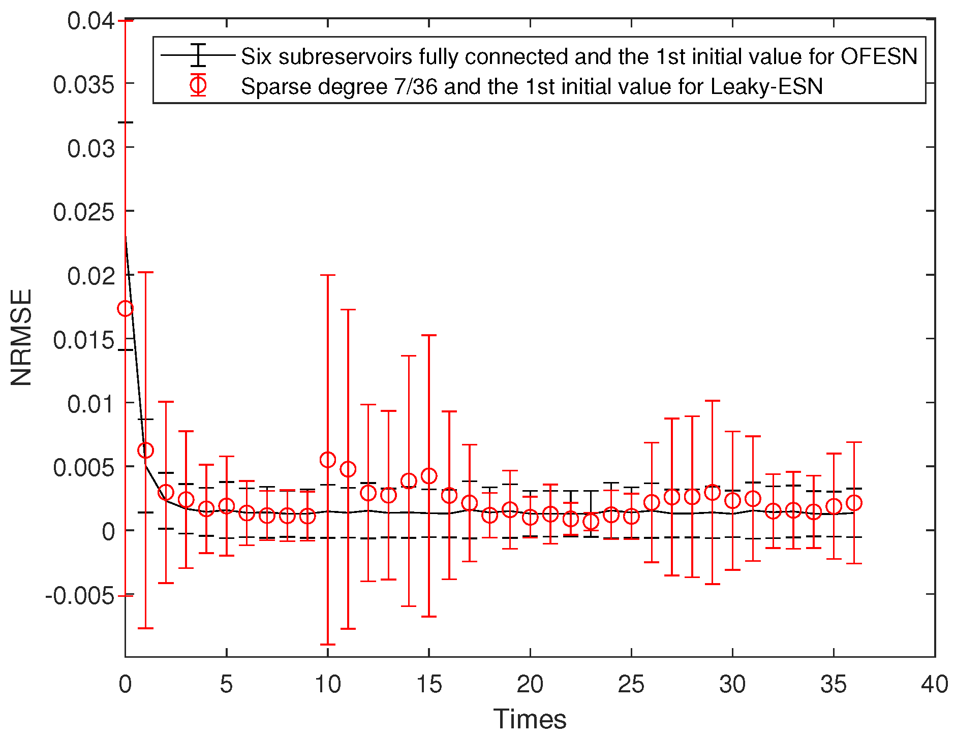
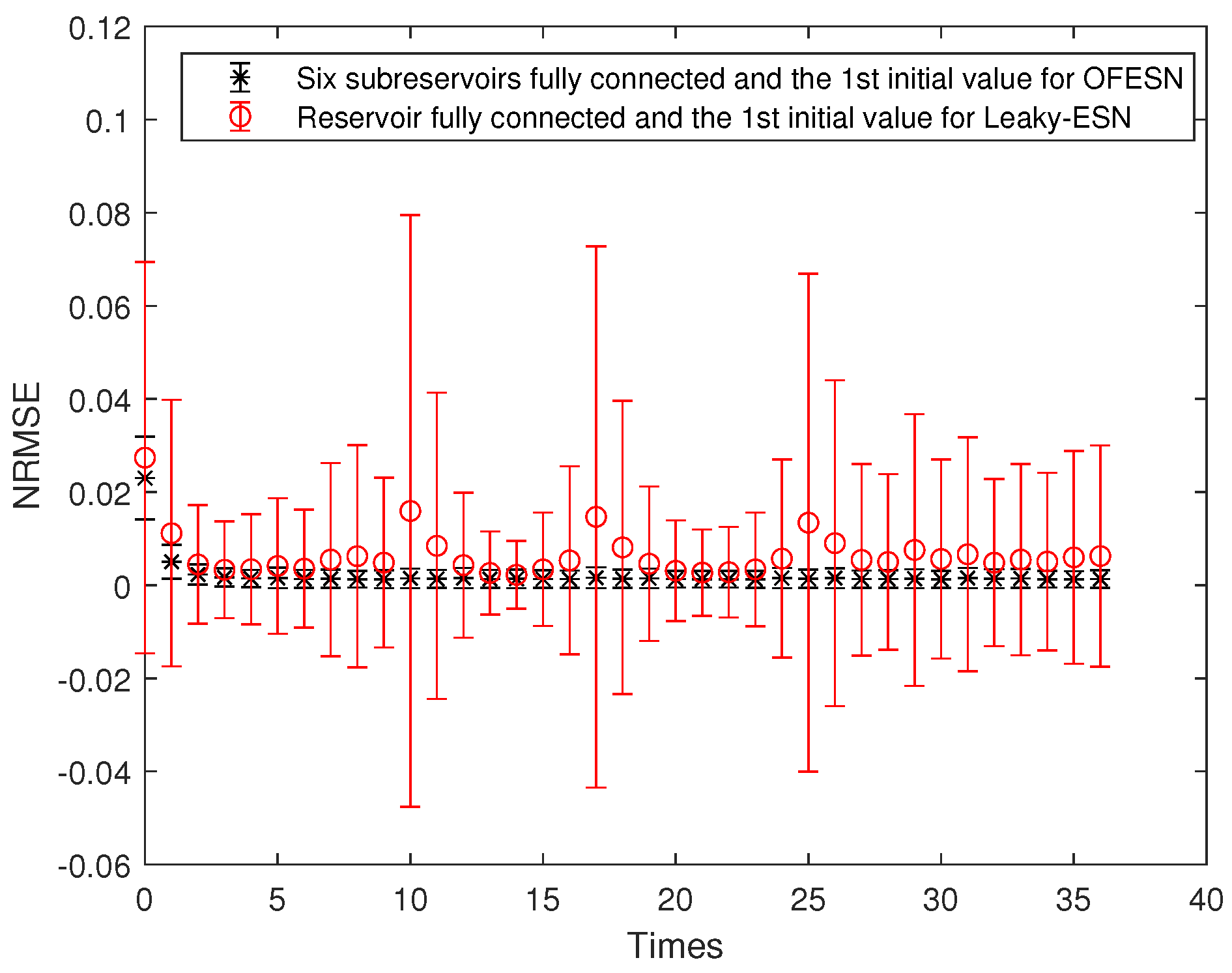
The sparse degree of each actual subreservoir is 1; that is, all the neurons in each actual subreservoir are connected, including interconnection and self-connection. The sparse degree of the virtual subreservoir is 1, and then the number of connections is 252. Thus, the corresponding sparse degree of Leaky-ESN should be set to $\frac{7}{36}$. In this case, the number of connected reservoir neurons of the OFESN is approximately the same as that of Leaky-ESN. Figure 12 shows the comparison between the OFESN and Leaky-ESN. Figure 13 shows the comparison between the OFESN with each subreservoir fully connected and Leaky-ESN with fully connected reservoir.

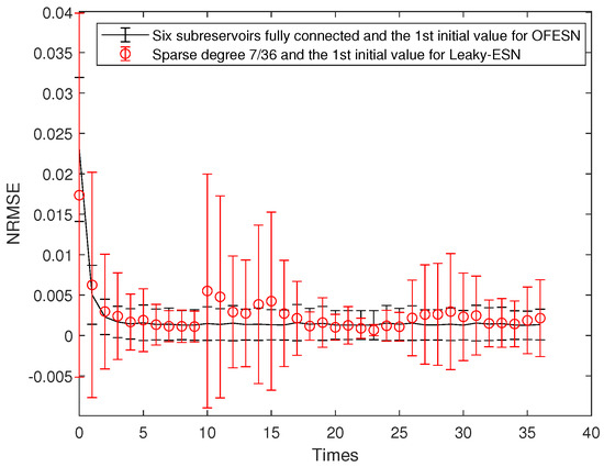
Figure 12. Comparison between the OFESN and Leaky-ESN under the first initial value and full connection.

Figure 13. Comparison between the OFESN with each subreservoir fully connected and Leaky-ESN with fully connected reservoir under the first initial value.

It can be seen that under the same conditions, compared with Leaky-ESN, the OFESN has higher prediction accuracy and smaller error fluctuation.

(ii).

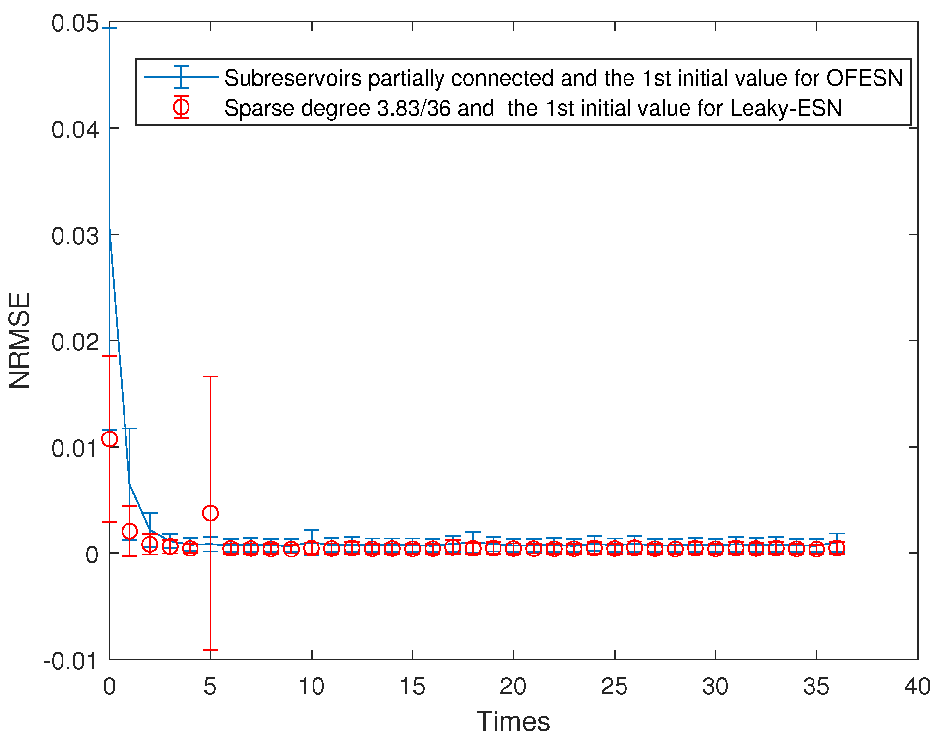
The first initial value case and the partially connected subreservoir (called Case 2)

The sparse degrees of the subreservoirs are selected as $\frac{3}{N_i}$$(i=1,2,\cdots ,5)$, $\frac{2}{N_6}$, and the sparse degree of the virtual subreservoir is $\frac{6}{N_7}$. Thus, the connection number of neurons in the whole reservoir is approximately as follows:

$$\begin{array}{c}\hfill N_{c\_partial\_6}=\sum _{i=1}^5{N}_i\ast N_i\ast \frac{3}{N_i}+N_6\ast N_6\ast \frac{2}{N_6}+N_7\ast N_7\end{array}$$

(29)

The corresponding approximate sparse degree of Leaky-ESN should be set to $\frac{3.83}{36}$. When the initial value is $[a\left(0\right),\overline{\rho }\left(0\right),S_i^{in}\left(0\right)]=[1;0.5\ast rand\left(1\right);0.15\ast rand\left(1\right)]$, the comparison between the OFESN and Leaky-ESN is shown in Figure 14. It can be seen that under the condition of different sparsity, the OFESN and Leaky-ESN have a similar prediction effect.

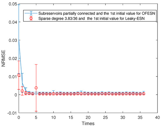
Figure 14. Comparison between the OFESN and Leaky-ESN under partial connection and the first initial value.

(iii).

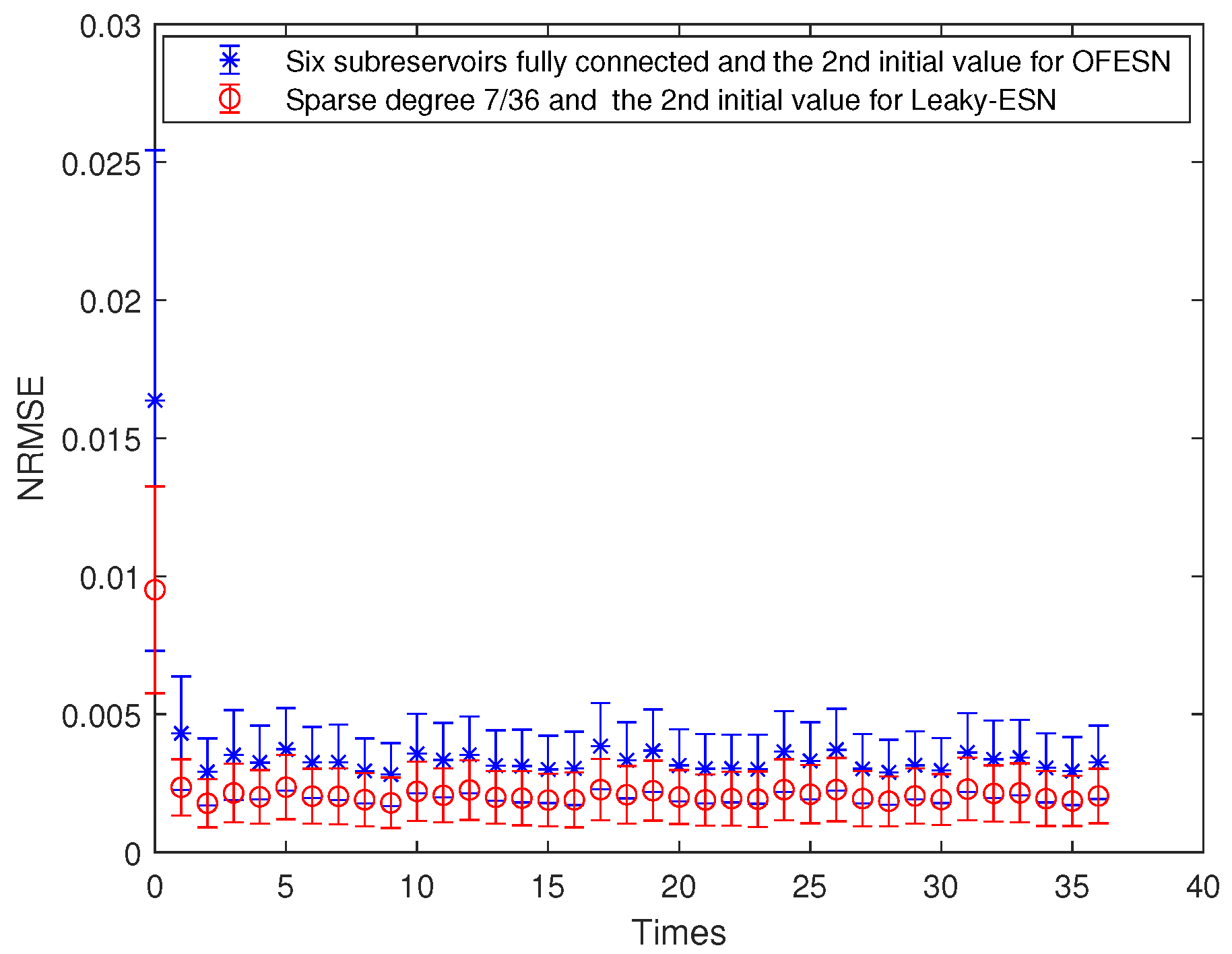
The second initial value case and the fully connected subreservoir (called Case 3)

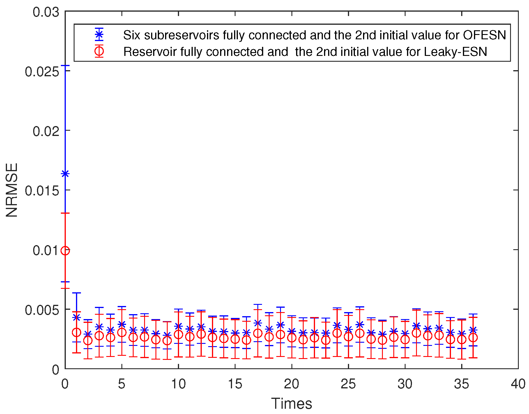
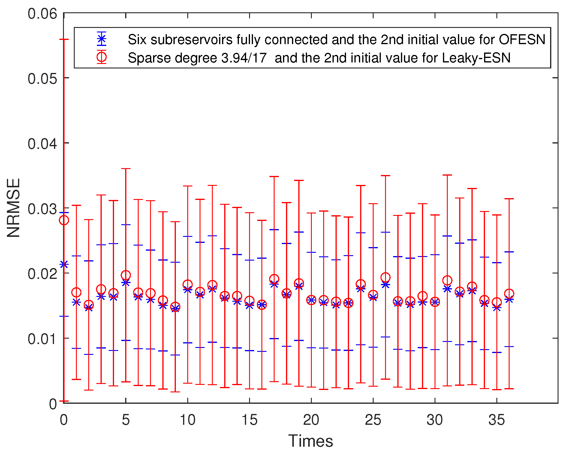
Each subreservoir is fully connected, and the corresponding sparse degree of Leaky-ESN should be set to $\frac{7}{36}$. Figure 15 shows the comparison between Leaky-ESN and the OFESN with each subreservoir fully connected at the second initial value. Figure 16 shows the comparison between the OFESN with each subreservoir fully connected and Leaky-ESN with fully connected reservoir. It can be seen that under the condition of full connection, Leaky-ESN has higher prediction accuracy and smaller error fluctuation compared with the OFESN.

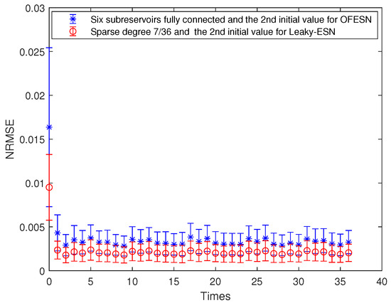
Figure 15. Comparison between the OFESN with each subreservoir fully connected and Leaky-ESN with sparse degree $\frac{7}{36}$ at the second initial value.

Figure 16. Comparison between the OFESN with each subreservoir fully connected and Leaky-ESN with the reservoir fully connected at the second initial value.

(iv).

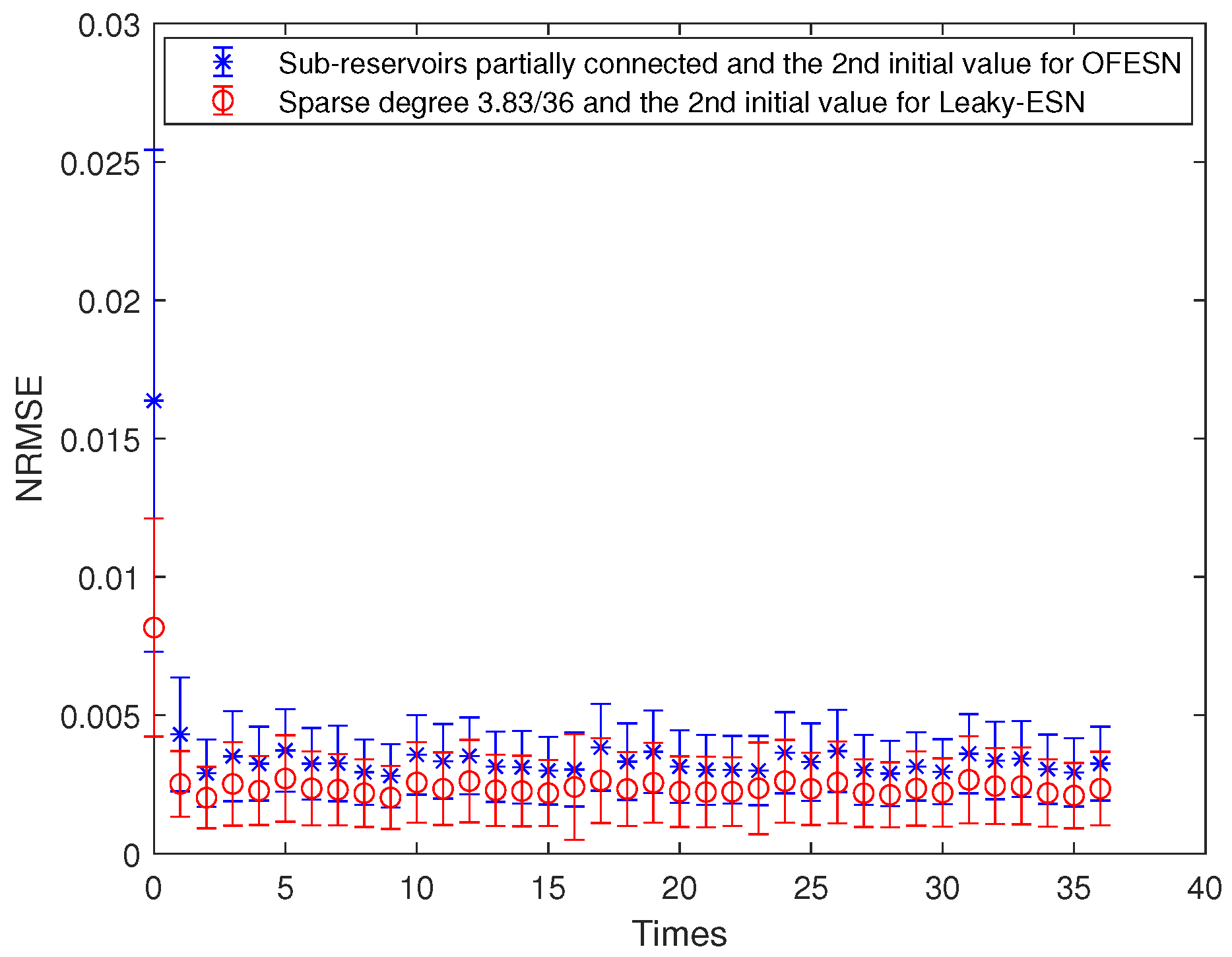
The second initial value case and the partially connected subreservoir (called Case 4)

The sparse degree of each actual subreservoir is $\frac{3}{N_i}(i=1,2,3,4,5)$, and $\frac{2}{N_6}$. The sparse degree of the virtual subreservoir is $\frac{6}{N_7}$. Thus, the corresponding sparse degree of leaky-ESN should be set to $\frac{3.83}{36}$. Figure 17 shows the comparison between the OFESN and Leaky-ESN at the second initial value and partially connected subreservoirs. It can be seen that under partial connection conditions, compared with Leaky-ESN, the OFESN has weaker prediction accuracy and greater error fluctuation.

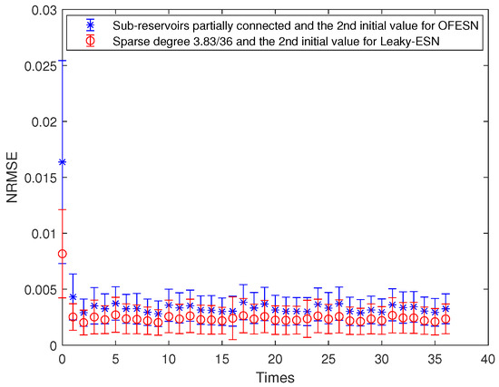
Figure 17. Comparison between the OFESN and Leaky-ESN under partial connection and the second initial value.

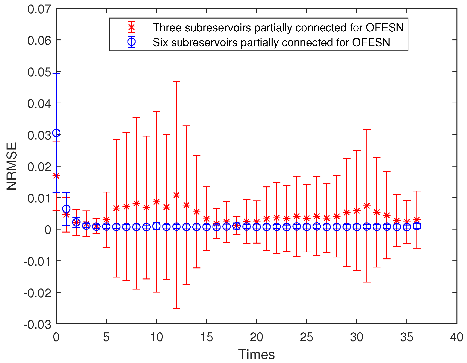
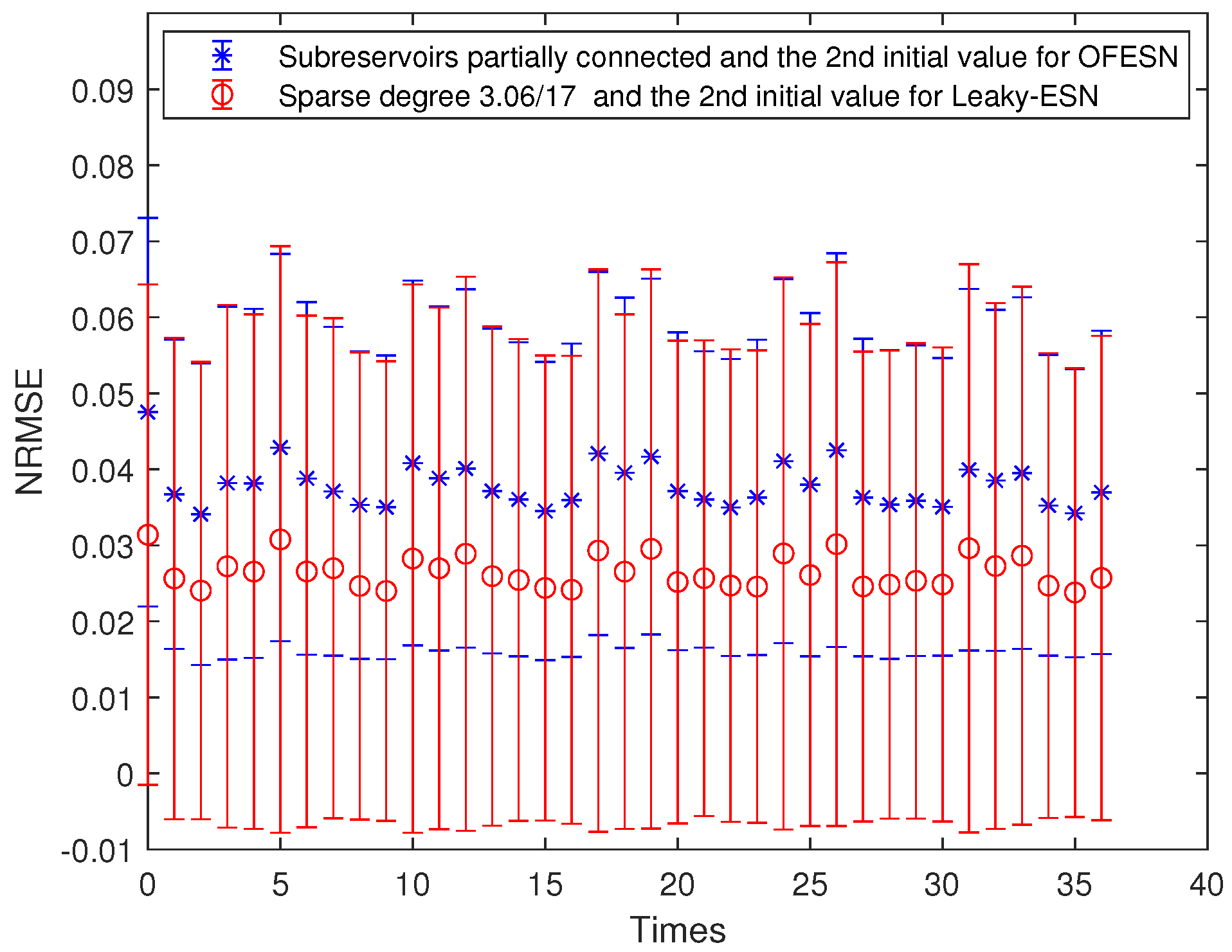
Under the same number of neurons in the whole reservoir, the performance comparison for the OFESN with a different number of subreservoirs is shown in Figure 18. In Figure 18, the red line with ∗ denotes the prediction error bars of the OFESN with three subreservoirs under the first initial value and subreservoirs partially connected, and the blue line with ∘ denotes the prediction error bars of the OFESN with six subreservoirs under the first initial value and subreservoirs partially connected.

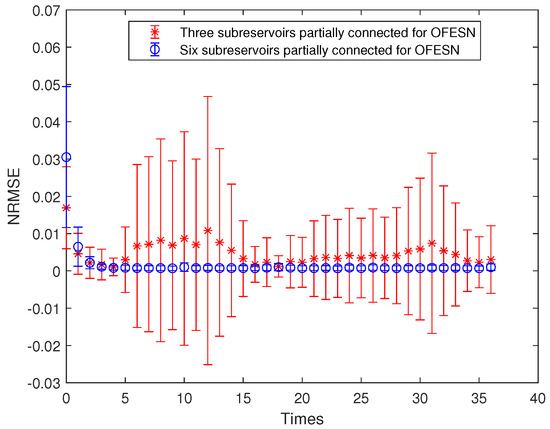
Figure 18. Comparison of the OFESN with a different number of subreservoirs under the first initial value and partial connection.

The predicted time series length is 500, and the run time is shown in Table 1. Table 2 shows the comparison of the core parameter ratio in the OFESN and Leaky-ESN. In Table 1, similar to Table 3 and Table 4, $NRMS{E}_{\_train}$ represents training error, $Tim{e}_{\_train}$ represents training time, $NRMS{E}_{\_test}$ represents testing error, and $Tim{e}_{\_test}$ represents testing time. In Table 2, similar to Table 5 and Table 6, a represents Leaky rate, $\rho$ represents spectral radius, and $S^{in}$ represents input scaling factor. As can be seen from Table 1, the training and test time of the OFESN are slightly better than Leaky-ESN; the training and test errors are both improved by an order of magnitude, and the prediction accuracy is improved by 98% at most. As can be seen from Table 2, a, $\rho$, and $S^{in}$ are closely related to the selection of initial values.

Table 1. Comparison of running time and NRMSE between the OFESN and Leaky-ESN.

		${\mathit{NRMSE}}_{\_\mathit{train}}$	${\mathit{Time}}_{\_\mathit{train}}$ (s)	${\mathit{NRMSE}}_{\_\mathit{test}}$	${\mathit{Time}}_{\_\mathit{test}}$ (s)
OFESN	Case1	$2.5609\times {10}^{-7}$	0.231060	$2.5282\times {10}^{-7}$	0.004107
	Case2	$6.3762\times {10}^{-7}$	0.234678	$7.2728\times {10}^{-7}$	0.004057
	Case3	$8.2226\times {10}^{-6}$	0.228521	$8.4277\times {10}^{-6}$	0.004182
	Case4	$4.7944\times {10}^{-6}$	0.232367	$5.2103\times {10}^{-6}$	0.004416
Leaky-ESN	Case1	$2.0096\times {10}^{-6}$	0.232815	$2.2874\times {10}^{-6}$	0.007072
	Case2	$2.9704\times {10}^{-6}$	0.246669	$3.1719\times {10}^{-6}$	0.006204
	Case3	$1.3395\times {10}^{-5}$	0.239171	$1.4666\times {10}^{-5}$	0.005308
	Case4	$1.3040\times {10}^{-5}$	0.276972	$1.4304\times {10}^{-5}$	0.006306

Table 2. Comparison of parameter values between OFESN and Leaky-ESN.

		a	$\mathit{\rho }$	${\mathit{S}}^{\mathit{in}}$
OFESN	Case 1	0.99972	0.30466	0.015876
	Case 2	0.99573	0.43532	0.219020
	Case 3	0.80057	0.59874	0.099303
	Case 4	0.80151	0.59847	0.096980
Leaky-ESN	Case 1	0.99979	0.40591	0.090287
	Case 2	0.99853	0.12769	0.095093
	Case 3	0.79942	0.59929	0.100000
	Case 4	0.80024	0.60003	0.100000

Table 3. Comparison of running time and NRMSE between the OFESN and Leaky-ESN.

		${\mathit{NRMSE}}_{\_\mathit{train}}$	${\mathit{Time}}_{\_\mathit{train}}$ (s)	${\mathit{NRMSE}}_{\_\mathit{test}}$	${\mathit{Time}}_{\_\mathit{test}}$ (s)
OFESN	Case1	$8.6111\times {10}^{-7}$	0.205972	$8.4250\times {10}^{-7}$	0.005496
	Case2	$2.8909\times {10}^{-5}$	0.214866	$2.8671\times {10}^{-5}$	0.004983
	Case3	$3.4598\times {10}^{-5}$	0.207253	$3.6116\times {10}^{-5}$	0.005006
	Case4	$6.3554\times {10}^{-5}$	0.251348	$6.6807\times {10}^{-5}$	0.004716
Leaky-ESN	Case1	$6.1811\times {10}^{-6}$	0.220781	$8.3576\times {10}^{-6}$	0.007218
	Case2	$2.1921\times {10}^{-5}$	0.202413	$6.4650\times {10}^{-5}$	0.005537
	Case3	$6.0361\times {10}^{-6}$	0.207606	$4.9683\times {10}^{-5}$	0.005591
	Case4	$2.2701\times {10}^{-5}$	0.216183	$2.5725\times {10}^{-4}$	0.005744

Table 4. Comparison of running time and NRMSE between the OFESN and Leaky-ESN for Mackey–Glass series.

		${\mathit{NRMSE}}_{\_\mathit{train}}$	${\mathit{Time}}_{\_\mathit{train}}$ (s)	${\mathit{NRMSE}}_{\_\mathit{test}}$	${\mathit{Time}}_{\_\mathit{test}}$ (s)
OFESN	Case1	$8.3616\times {10}^{-8}$	0.535822	$6.0156\times {10}^{-8}$	0.059386
	Case2	$6.6978\times {10}^{-8}$	0.231891	$8.2199\times {10}^{-8}$	0.066284
	Case3	$1.6348\times {10}^{-7}$	0.237385	$6.4672\times {10}^{-8}$	0.046180
	Case4	$1.3460\times {10}^{-7}$	0.237897	$5.4552\times {10}^{-8}$	0.046180
Leaky-ESN	Case1	$6.093\times {10}^{-7}$	0.238008	$6.9946\times {10}^{-7}$	0.076255
	Case2	$1.8484\times {10}^{-7}$	0.233209	$2.1197\times {10}^{-7}$	0.055636
	Case3	$1.1278\times {10}^{-7}$	0.239115	$1.4215\times {10}^{-7}$	0.055965
	Case4	$1.9905\times {10}^{-7}$	0.235569	$2.2779\times {10}^{-7}$	0.056949

Table 5. Comparison of parameter values between the OFESN and Leaky-ESN.

		a	$\mathit{\rho }$	${\mathit{S}}^{\mathit{in}}$
OFESN	Case 1	0.95811	0.32002	0.017681
	Case 2	0.99767	0.17067	0.080665
	Case 3	0.72506	0.29053	0.071419
	Case 4	0.80024	0.59986	0.098906
Leaky-ESN	Case 1	1.0008	0.23961	0.08112
	Case 2	0.97694	0.027551	0.13631
	Case 3	0.79864	0.59956	0.100000
	Case 4	0.79933	0.59911	0.100000

Table 6. Comparison of parameter values between the OFESN and Leaky-ESN for Mackey–Glass series.

		a	$\mathit{\rho }$	${\mathit{S}}^{\mathit{in}}$
OFESN	Case 1	0.99923	0.36061	0.083281
	Case 2	1.00020	0.41180	0.14214
	Case 3	0.79966	0.60101	0.095925
	Case 4	0.80077	0.59993	0.098408
Leaky-ESN	Case 1	0.99521	0.32643	0.094922
	Case 2	1.00150	0.43965	0.044478
	Case 3	0.80458	0.59322	0.100000
	Case 4	0.79861	0.60050	0.100000

4.1.3. The Reservoir with 17 Neurons

In order to test the performance of the OFESN when the reservoir contains only a small number of neurons, we select the total number of neurons in the reservoir $N=17$ in the following simulation. Assuming that the reservoir is divided into 6 actual subreservoirs, $N_i=3$$(i=1,2,\cdots ,5)$, $N_6=2$, and then the number of neurons in the virtual reservoir is $N_7=6$. The performance of the OFESN is tested on the case of the reservoir neurons with different connections and two different initial values of the reservoir parameters.

(i).

The first initial value case and the fully connected subreservoir (called Case 1)

The sparse degree of each actual subreservoirs of the OFESN is set to 1; that is, it is fully connected. The sparse degree of the virtual subreservoir is $\frac{3}{6}$. Thus, the reservoir of the OFESN is equivalent to having 67 internal connection weights. Corresponding to Leaky-ESN, its sparse degree is $\frac{3.94}{17}$. Figure 19 shows the performance of the OFESN and Leaky-ESN. It can be seen that the prediction performance of the OFESN is significantly better than Leaky-ESN, and it has smaller error fluctuation.

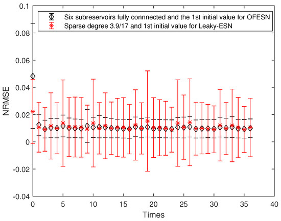
Figure 19. Comparison between the OFESN with each subreservoir fully connected and Leaky-ESN under the first initial value.

(ii).

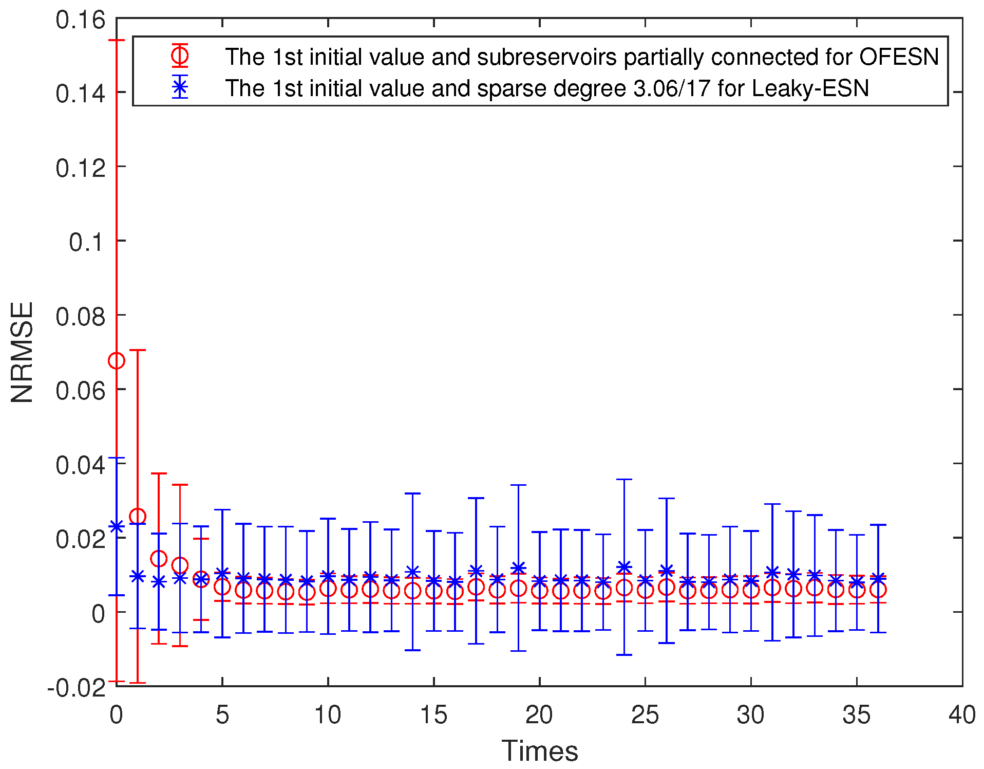
The first initial value case and the partially connected subreservoir (called Case 2)

The sparse degree of each subreservoir is set to $\frac{2}{N_i}(i=1,2,3,4,5,6)$, $\frac{3}{N_7}$, respectively, and is equivalent to 52 internal connection weights. Thus, the corresponding sparse degree of leaky-ESN should be set to $\frac{3.06}{17}$. The performance comparison between the OFESN and leaky-ESN is shown in Figure 20. It can be seen that in the whole training process, the prediction performance of Leaky-ESN is better than that of the OFESN, and the error fluctuation is smaller.

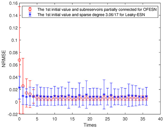
Figure 20. Comparison between the OFESN with each subreservoir partially connected and Leaky-ESN under the first initial value.

(iii).

The second initial value case and the fully connected subreservoir (called Case 3)

The sparse degree of each actual subreservoir is set to 1; that is, it is fully connected. The sparse degree of the virtual subreservoir is $\frac{3}{6}$, which is equivalent to having 67 internal connection weights in the whole reservoir., corresponding to Leaky-ESN, and its sparse degree is $\frac{3.94}{17}$. Figure 21 shows the performance comparison between the OFESN and Leaky-ESN. It can be seen that the OFESN is slightly better than Leaky-ESN in terms of prediction accuracy and error fluctuation.

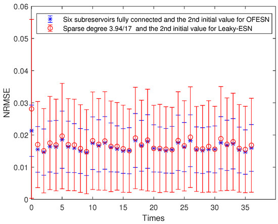
Figure 21. Comparison between the OFESN with each subreservoir fully connected and Leaky-ESN under the first initial value.

(iv).

The second initial value case and the partially connected subreservoir (called Case 4)

The sparse degree of each actual subreservoir is set to $2/N_i$$(i=1,2,\cdots ,6)$; that is, it is partially connected. The sparse degree of the virtual subreservoir is $\frac{3}{6}$, which is equivalent to having 52 internal connection weights in the whole reservoir, which corresponds to Leaky-ESN, and its sparse degree is $\frac{3.06}{17}$. Figure 22 shows the performance comparison between the OFESN and Leaky-ESN.

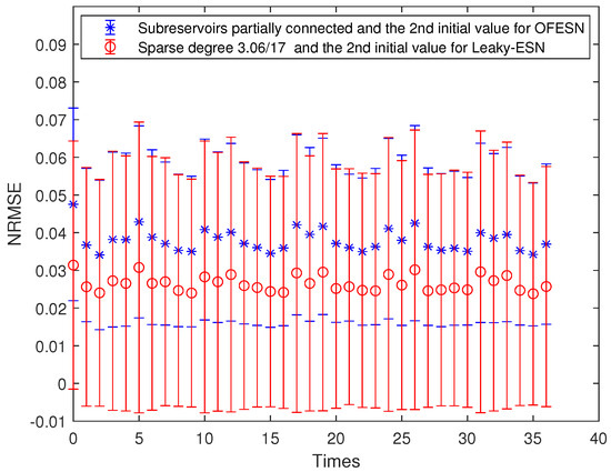
Figure 22. Comparison between the OFESN and Leaky-ESN under partial connection and the second initial value.

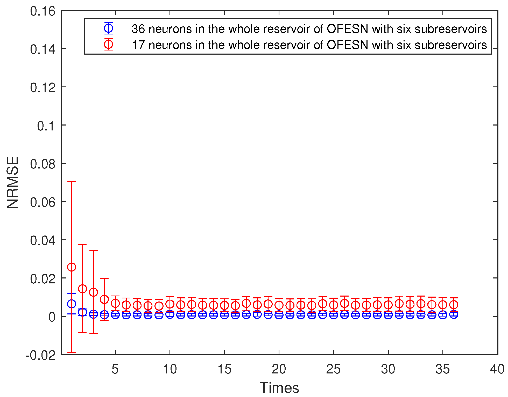
Figure 23 shows the performance comparison between the OFESN with 36 neurons and the OFESN with 17 neurons in the case of the first initial value and partially connected subreservoirs. The predicted time series length is 20,000, and run time is shown in Table 3. Table 5 shows the comparison of the core parameter ratio in the OFESN and Leaky-ESN. As can be seen from Table 3, the training and test time of the OFESN is slightly better than Leaky-ESN; the training and test errors are both improved by an order of magnitude, and the prediction accuracy is improved by 96% at most. As can be seen from Table 5, a, $\rho$, and $S^{in}$ are closely related to the selection of initial values.

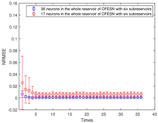
Figure 23. Comparison between the OFESN with each subreservoir fully connected and Leaky-ESN with fully connected reservoir under the first initial value.

4.1.4. Analysis of the Simulation Results

We can see from the simulation figures that the prediction performance of the OFESN with the same number of internal connection weights is better than that of Leaky-ESN under more cases. Even if the prediction performance of the OFESN with the same number of connection weights is similar to that of the ESN, the prediction error volatility of the OFESN is much smaller than that of Leaky-ESN. In addition, we give comparisons between the OFESN with each subreservoir fully connected and Leaky-ESN with full connection, shown in Figure 6, Figure 9, Figure 13 and Figure 16, and the OFESN with each subreservoir fully connected has a better performance and less error fluctuation than Leaky-ESN with full connection. We can see from Figure 23 that the OFESN with 36 neurons and 3 subreservoirs has a prediction performance closer to the OFESN with 17 neurons and 6 subreservoirs in the whole reservoir. Thus, we can say, when the number of neurons is small, the greater the number of subreservoirs, the greater the number of neurons in the whole reservoir by adding a virtual reservoir. In a word, the OFESN has more stable performance and shorter run time.

4.2. Mackey–Glass Chaotic Time Series

The Mackey–Glass chaotic time series (MGS) is a classic nonlinear dynamical system, commonly used in fields such as time series analysis, signal processing, and chaos theory. For example, the Mackey–Glass equation can be used to describe the fluctuations and trends in market prices in economics and study the biological clock and rhythmic behavior within organisms in biology. The Mackey–Glass equation can be represented as

$$g(\theta +1)=g\left(\theta \right)+\Delta T(\frac{pg(t-\frac{\tau }{\Delta T})}{1+g{(t-\frac{\tau }{\Delta T})}^{10}}+qg\left(\theta \right))$$

(30)

where $p=0.2$, $\tau =17$, $q=-0.1$, $\Delta T=0.1$. $\tau$ denotes the delay factor, and the sequence has chaotic properties when $\tau >16.8$. We normalize the dataset by the min-max scaling method so that all the data are between 0 and 1. We split the time series dataset by using $70\%$ of it for training purposes, $20\%$ for validation purposes, and the remaining $10\%$ for testing purposes. The first 100 samples are discarded during training to guarantee that the system is not affected by the initial transient, in accordance with the echo property. According to Equations (23) and (24), we generate 40,000 data samples, which are divided into three parts: 20,000 training samples, 10,000 testing sample points, and 100 initial washing out samples. The predicted time series length is 20,000, and the run time is shown in Table 4. Table 6 shows the comparison of core parameter ratio in the OFESN and Leaky-ESN.

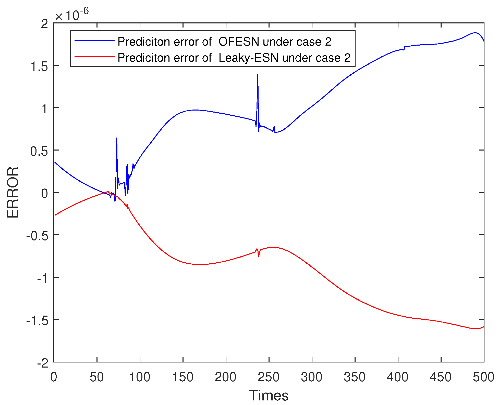
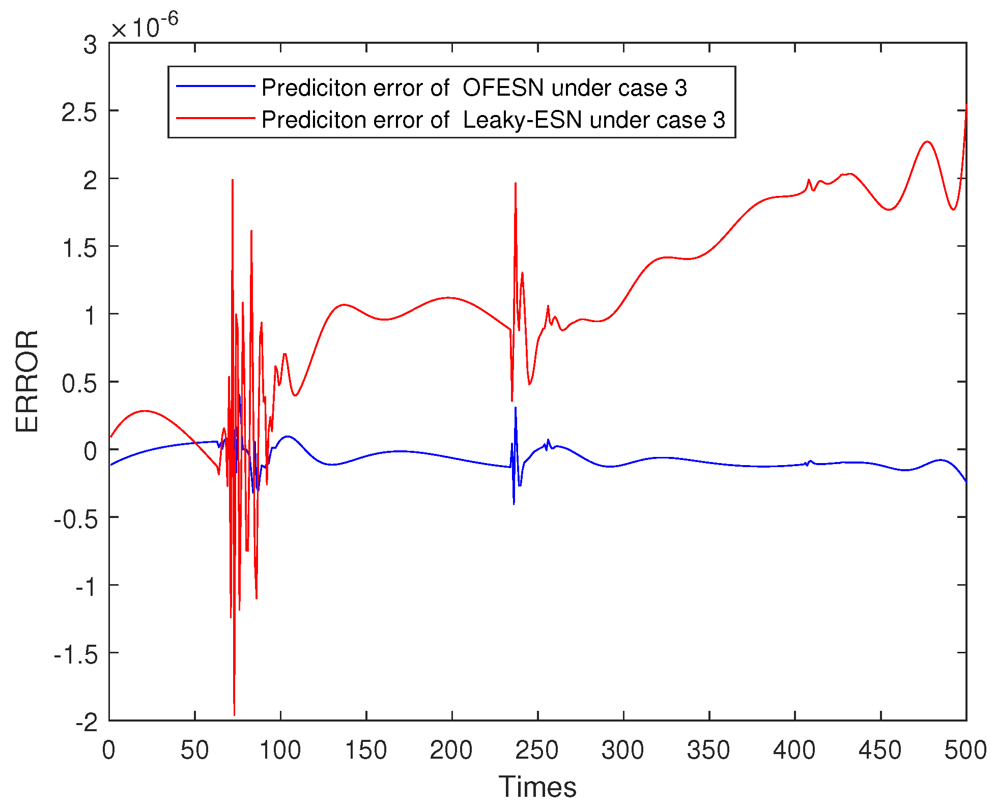
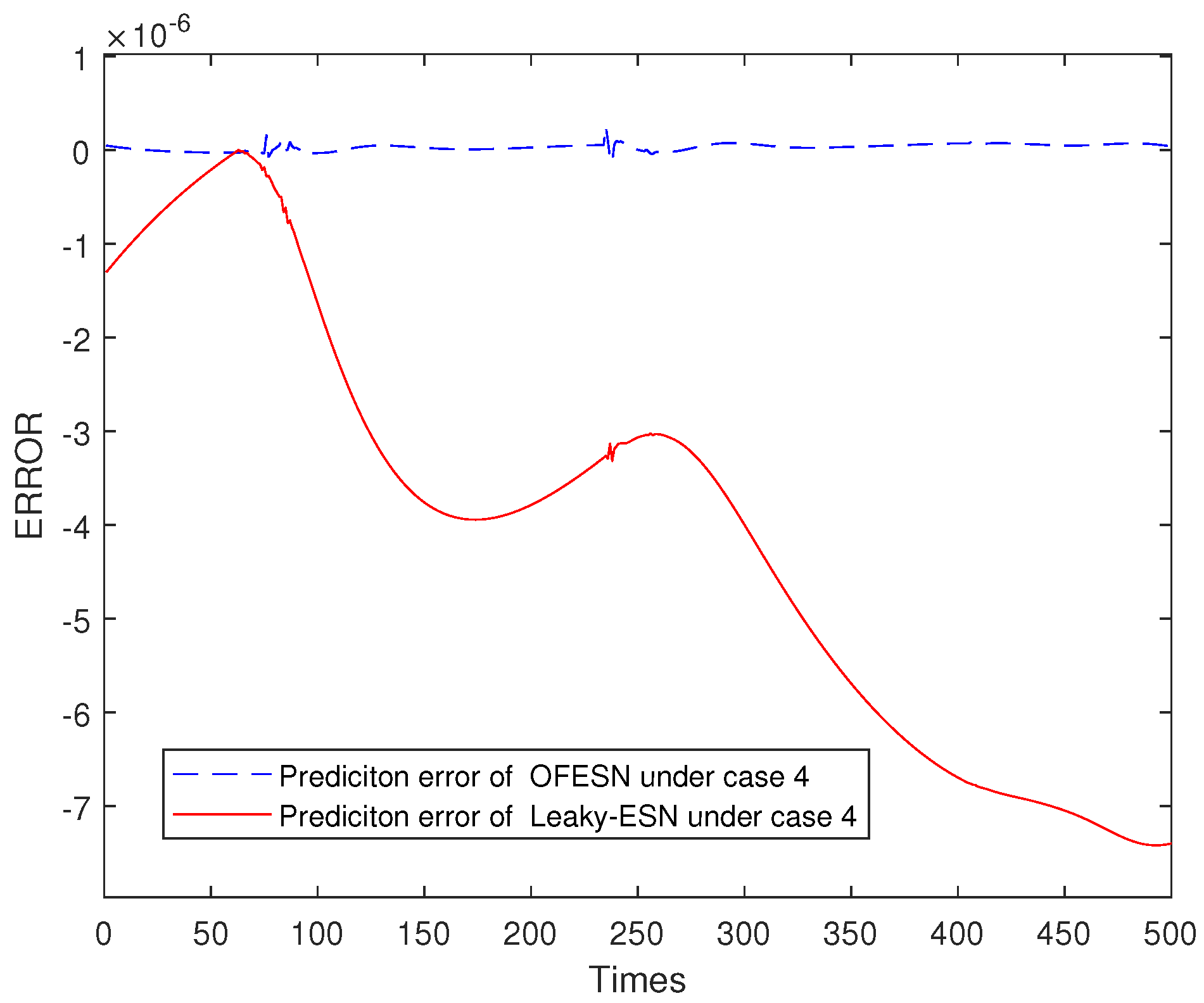
Figure 24, Figure 25, Figure 26 and Figure 27 shows the comparison of prediction error results of the OFESN and Leaky-ESN in different cases. As can be seen from the figure, in cases 1, 2, and 4, the prediction error of Leaky-ESN is significantly better than that of the OFESN, and it tends to converge, while the OFESN tends to diverge. In case 3, the prediction effect of the OFESN is better than Leaky-ESN. As can be seen from Table 4, the training and test time of the OFESN is slightly better than Leaky-ESN; the training and test errors are both improved by an order of magnitude, and the prediction accuracy is improved by 98% at most. As can be seen from Table 6, a, $\rho$, and $S^{in}$ are closely related to the selection of initial values.

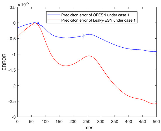
Figure 24. Error result based on the OFESN and Leaky-ESN for Mackey–Glass.

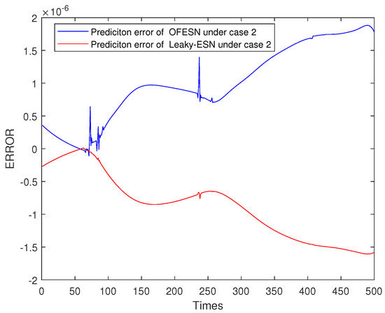
Figure 25. Error result based on the OFESN and Leaky-ESN for Mackey–Glass.

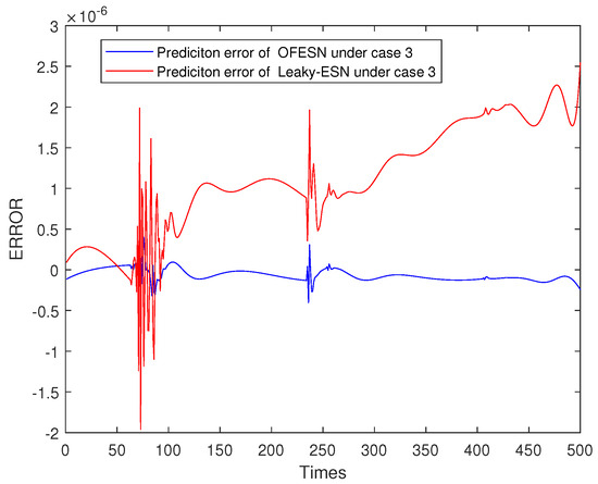
Figure 26. Error result based on the OFESN and Leaky-ESN for Mackey–Glass.

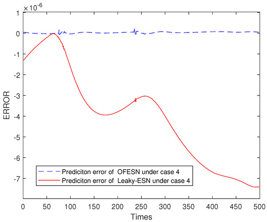
Figure 27. Error result based on the OFESN and Leaky-ESN for Mackey–Glass.

5. Conclusions

This paper proposed a new multireservoir echo state network, namely the OFESN. The OFESN can transform the connections of a single reservoir into the connections of subreservoirs by their master neurons, greatly reducing the coupling connections between neurons in a reservoir, further increasing sparse degree, and reducing information redundancy. Compared with Leaky-ESN network, the OFESN network greatly reduces the internal coupling and correlation between different subreservoirs. Without increasing the number of neurons in the reservoir, introducing a sparse connection between the master neurons is actually equivalent to greatly increasing the number of neurons, especially the number of neurons with great dissimilarity. Therefore, when the number of neurons in each actual subreservoir is small and the number of subreservoirs is large, it is equivalent to obtaining more reservoir neurons and ensuring the dissimilarity of neuron states, which improves the prediction accuracy of Leaky-ESN and greatly reduces the amount of calculation. Prediction accuracy improved by 98% in some cases. However, there are some limitations to the OFESN and Leaky-ESN. The gradient descent optimization method is used to optimize parameters with constraint conditions (echo state characteristic conditions), which is sensitive to the initial value selection of parameters and cannot guarantee global optimization. Therefore, in the future, we will find a suitable swarm intelligence optimization algorithm to optimize its parameters to eliminate the impact of the initial parameter values. The performance comparison between the OFESN and LEAKY-ESN is not a comparison between the optimal performance of the two models but a comparison under the same parameters and equivalent conditions.

References

- Beritelli, F.; Capizzi, G.; Sciuto, G.L.; Napoli, C.; Tramontana, E.; Woźniak, M. Reducing interferences in wireless communication systems by mobile agents with recurrent neural networks-based adaptive channel equalization. Photonics Applications in Astronomy, Communications, Industry, and High-Energy Physics Experiments 2015. In Proceedings of the XXXVI Symposium on Photonics Applications in Astronomy, Communications, Industry, and High-Energy Physics Experiments (Wilga 2015), Wilga, Poland, 25 May 2015; Volume 9662, pp. 497–505. [Google Scholar]
- Jaeger, H. The “echo state” approach to analysing and training recurrent neural networks-with an erratum note. Bonn Ger. Ger. Natl. Res. Cent. Inf. Technol. GMD Tech. Rep. 2001, 148, 13. [Google Scholar]
- Jaeger, H.; Haas, H. Harnessing nonlinearity: Predicting chaotic systems and saving energy in wireless communication. Science 2004, 304, 78–80. [Google Scholar] [CrossRef]
- Jaeger, H. Tutorial on Training Recurrent Neural Networks, Covering BPPT, RTRL, EKF and the “Echo State Network” Approach; German National Research Center for Information Technology: Sankt Augustin, Germany, 2002. [Google Scholar]
- Soliman, M.; Mousa, M.A.; Saleh, M.A.; Elsamanty, M.; Radwan, A.G. Modelling and implementation of soft bio-mimetic turtle using echo state network and soft pneumatic actuators. Sci. Rep. 2021, 11, 12076. [Google Scholar] [CrossRef] [PubMed]
- Wootton, A.J.; Taylor, S.L.; Day, C.R.; Haycock, P.W. Optimizing echo state networks for static pattern recognition. Cogn. Comput. 2017, 9, 391–399. [Google Scholar] [CrossRef]
- Mahmoud, T.A.; Abdo, M.I.; Elsheikh, E.A.; Elshenawy, L.M. Direct adaptive control for nonlinear systems using a TSK fuzzy echo state network based on fractional-order learning algorithm. J. Frankl. Inst. 2021, 358, 9034–9060. [Google Scholar] [CrossRef]
- Wang, Q.; Pan, Y.; Cao, J.; Liu, H. Adaptive Fuzzy Echo State Network Control of Fractional-Order Large-Scale Nonlinear Systems With Time-Varying Deferred Constraints. IEEE Trans. Fuzzy Syst. 2023, 1–15. [Google Scholar] [CrossRef]
- Gao, R.; Du, L.; Duru, O.; Yuen, K.F. Time series forecasting based on echo state network and empirical wavelet transformation. Appl. Soft Comput. 2021, 102, 107111. [Google Scholar] [CrossRef]
- Bai, Y.; Liu, M.D.; Ding, L.; Ma, Y.J. Double-layer staged training echo-state networks for wind speed prediction using variational mode decomposition. Appl. Energy 2021, 301, 117461. [Google Scholar] [CrossRef]
- Tian, Z. Echo state network based on improved fruit fly optimization algorithm for chaotic time series prediction. J. Ambient Intell. Humaniz. Comput. 2022, 13, 3483–3502. [Google Scholar] [CrossRef]
- Ribeiro, G.T.; Santos, A.A.P.; Mariani, V.C.; dos Santos Coelho, L. Novel hybrid model based on echo state neural network applied to the prediction of stock price return volatility. Expert Syst. Appl. 2021, 184, 115490. [Google Scholar] [CrossRef]
- Qiao, J.; Li, F.; Han, H.; Li, W. Growing echo-state network with multiple subreservoirs. IEEE Trans. Neural Netw. Learn. Syst. 2016, 28, 391–404. [Google Scholar] [CrossRef] [PubMed]
- Huang, J.; Li, Y.; Shardt, Y.A.; Qiao, L.; Shi, M.; Yang, X. Error-driven chained multiple-subnetwork echo state network for time-series prediction. IEEE Sens. J. 2022, 22, 19533–19542. [Google Scholar] [CrossRef]
- Ma, Q.; Chen, E.; Lin, Z.; Yan, J.; Yu, Z.; Ng, W.W. Convolutional multitimescale echo state network. IEEE Trans. Cybern. 2019, 51, 1613–1625. [Google Scholar] [CrossRef] [PubMed]
- Gallicchio, C.; Micheli, A. Deep reservoir neural networks for trees. Inf. Sci. 2019, 480, 174–193. [Google Scholar] [CrossRef]
- Na, X.; Zhang, M.; Ren, W.; Han, M. Multi-step-ahead chaotic time series prediction based on hierarchical echo state network with augmented random features. IEEE Trans. Cogn. Dev. Syst. 2022, 15, 700–711. [Google Scholar] [CrossRef]
- Wang, H.; Wu, Q.J.; Wang, D.; Xin, J.; Yang, Y.; Yu, K. Echo state network with a global reversible autoencoder for time series classification. Inf. Sci. 2021, 570, 744–768. [Google Scholar] [CrossRef]
- Lun, S.X.; Yao, X.S.; Qi, H.Y.; Hu, H.F. A novel model of leaky integrator echo state network for time-series prediction. Neurocomputing 2015, 159, 58–66. [Google Scholar] [CrossRef]
- Lun, S.; Zhang, Z.; Li, M.; Lu, X. Parameter Optimization in a Leaky Integrator Echo State Network with an Improved Gravitational Search Algorithm. Mathematics 2023, 11, 1514. [Google Scholar] [CrossRef]
- Ren, W.; Ma, D.; Han, M. Multivariate Time Series Predictor With Parameter Optimization and Feature Selection Based on Modified Binary Salp Swarm Algorithm. IEEE Trans. Ind. Inform. 2022, 19, 6150–6159. [Google Scholar] [CrossRef]
- Hu, H.; Wang, L.; Tao, R. Wind speed forecasting based on variational mode decomposition and improved echo state network. Renew. Energy 2021, 164, 729–751. [Google Scholar] [CrossRef]
- Wainrib, G.; Galtier, M.N. A local echo state property through the largest Lyapunov exponent. Neural Netw. 2016, 76, 39–45. [Google Scholar] [CrossRef] [PubMed]
- Gallicchio, C.; Micheli, A. Echo state property of deep reservoir computing networks. Cogn. Comput. 2017, 9, 337–350. [Google Scholar] [CrossRef]
- Yang, C.; Qiao, J.; Ahmad, Z.; Nie, K.; Wang, L. Online sequential echo state network with sparse RLS algorithm for time series prediction. Neural Netw. 2019, 118, 32–42. [Google Scholar] [CrossRef]
- Gallicchio, C.; Micheli, A.; Pedrelli, L. Deep reservoir computing: A critical experimental analysis. Neurocomputing 2017, 268, 87–99. [Google Scholar] [CrossRef]
- Wu, Z.; Li, Q.; Zhang, H. Chain-structure echo state network with stochastic optimization: Methodology and application. IEEE Trans. Neural Netw. Learn. Syst. 2021, 33, 1974–1985. [Google Scholar] [CrossRef] [PubMed]
- Jaeger, H.; Lukoševičius, M.; Popovici, D.; Siewert, U. Optimization and applications of echo state networks with leaky-integrator neurons. Neural Netw. 2007, 20, 335–352. [Google Scholar] [CrossRef] [PubMed]
Disclaimer/Publisher’s Note: The statements, opinions and data contained in all publications are solely those of the individual author(s) and contributor(s) and not of MDPI and/or the editor(s). MDPI and/or the editor(s) disclaim responsibility for any injury to people or property resulting from any ideas, methods, instructions or products referred to in the content. |
© 2023 by the authors. Licensee MDPI, Basel, Switzerland. This article is an open access article distributed under the terms and conditions of the Creative Commons Attribution (CC BY) license (https://creativecommons.org/licenses/by/4.0/).