Abstract
In speed skating, the number of strokes in the first 100 m section serves as an important metric of final performance. However, the conventional method, relying on human vision, has limitations in terms of real-time counting and accuracy. This study presents a solution for counting strokes in the first 100 m of a speed skating race, aiming to overcome the limitations of human vision. The method uses image recognition technology, specifically MediaPipe, to track key body joint coordinates during the skater’s motion. These coordinates are calculated into important body angles, including those from the shoulder to the knee and from the pelvis to the ankle. To quantify the skater’s motion, the study introduces generalized labeling logic (GLL), a key index derived from angle data. The GLL signal is refined using Gaussian filtering to remove noise, and the number of inflection points in the filtered GLL signal is used to determine the number of strokes. The method was designed with a focus on frontal videos and achieved an excellent accuracy of 99.91% when measuring stroke counts relative to actual counts. This technology has great potential for enhancing training and evaluation in speed skating.
1. Introduction
Speed skating is a highly competitive sport that demands a combination of skill, technique, and endurance. Athletes undergo rigorous training programs to develop their strength, endurance, and technique for optimal performance. Motion analysis technology has become increasingly vital in speed skating events, enabling coaches and trainers to scrutinize athletes’ movements in detail. Studies employing motion analysis in speed skating include [1,2]. These data are crucial for identifying areas requiring improvement in technique and facilitating the creation of more effective, personalized training programs. Furthermore, motion analysis technology allows for the monitoring of an athlete’s progress over time, helping them set realistic goals and measure their development. Even minor adjustments in technique can significantly impact speed skating performance, necessitating access to precise and detailed movement data.
This technology serves not only to enhance performance but also to minimize the risk of injuries in speed skating events. By analyzing athletes’ movements, coaches can identify actions linked to a higher injury risk and develop strategies to reduce these risks. In summary, motion analysis technology is indispensable in speed skating, aiding coaches and trainers in pinpointing areas for improvement, developing tailored training programs, monitoring progress, and reducing the risk of injuries. Access to accurate and detailed movement data is fundamental for achieving optimal performance and ensuring the safety of athletes in this highly competitive sport.
Speed skating is a competitive sport in which skaters compete on an ice track to cover a set distance faster than their opponents. The objective is to reduce time, and rankings are determined solely based on an individual’s time, which often relies on small time differences. Therefore, various factors are used to improve the recording of times. De Koning et al.’s paper [3] states that the skating position, amount of work at push-off, klapskates, and push-off directionality are technical factors that affect speed skating performance. An important parameter is the number of strokes in the first 100 m of the straightaway after the start. Kim et al.’s paper [4] states that there is a positive correlation between the number of strokes and the final record in the 100 m section after the start, and a study by de Boer et al. [5] mentioned that stroke frequency can be judged as the major regulator of speed. Each side-to-side movement of the skater’s body is considered a stroke. Lee et al. [6] revealed that a higher stroke frequency in the first 100 m was positively correlated with improved performance. Therefore, increasing the number of strokes in the first 100 m of the straightaway is crucial for reducing the final recorded time. However, existing methods of manually calculating strokes have limitations such as being cumbersome and prone to error. An automation of this process can solve many problems with the conventional system and improve the performance of the athletes.
In this study, we addressed the problem of accurately measuring the number of strokes in the first 100 m of the sprint section during speed skating. The system captures the main joint points in a sprint video and uses their three-dimensional (3D) coordinates. MediaPipe Pose was used to obtain relatively accurate results. We emphasized the importance of maintaining accuracy and consistency in the measurement results. The method was devised to be simple and easy to learn. The system allows measurements to be obtained using conventional two-dimensional (2D) cameras, which eliminates the necessity for additional equipment. Videos captured from various angles can be considered when measuring player strokes. However, ensuring accuracy and consistency in a limited shooting environment is critical, even if videos cannot be captured from all angles. Therefore, the system is designed under the assumption that the number of strokes is measured using only videos captured from the front of the measurement target.
2. Related Works
Over the past few decades, there has been a significant increase in the use of motion analysis technology in sports events to improve athlete performance. Motion analysis involves using sensors, cameras, and other equipment to collect data on an athlete’s movements, which are then analyzed to identify areas for improvement. The aim of this section is to summarize the research trends related to performance improvement through motion analysis in sports events.
First, a macroscopic view will be taken of the relationship between the sports field and various analysis technologies by examining research trends in athlete-personalized training and performance improvement using exercise analysis technology and AI. One of the primary research trends in this area is the use of motion analysis technology to identify key performance indicators (KPIs) in athletes [7,8,9]. KPIs are specific metrics that are used to evaluate an athlete’s performance such as speed, power, and agility. By using motion analysis technology, coaches and trainers can identify which KPIs are most important for a given sport or athlete and develop training programs that focus on improving these areas.
Another important research trend in this area is the use of motion analysis to monitor athlete progress over time [10,11,12]. By collecting data on an athlete’s movements during training and competition, coaches and trainers can track their progress and identify areas where they need to improve. This can help athletes set realistic goals and measure their progress towards achieving them.
In recent years, there has been a growing interest in the use of machine learning and artificial intelligence (AI) to analyze motion data in sports events [13,14,15]. Machine learning algorithms can be used to identify patterns in large datasets, which can help coaches and trainers make more informed decisions about training and strategy. For example, machine learning algorithms can be used to identify specific movements that are associated with an increased risk of injury, allowing coaches and trainers to develop strategies to minimize this risk.
Another important area of research in this field is the use of motion analysis to develop customized training programs for individual athletes [16,17]. Coaches and trainers can create customized training programs by analyzing an athlete’s movements and identifying areas for improvement, meeting the athlete’s specific needs. This can help maximize the effectiveness of training and improve overall performance.
Finally, there has been a growing interest in the use of motion analysis technology to improve performance in team sports [18,19,20]. In team sports, it can be challenging to identify the individual contributions of each athlete to the team’s overall performance. However, by using motion analysis technology, coaches and trainers can analyze the movements of individual athletes and identify areas where they can contribute more effectively to the team.
Consequently, the use of motion analysis technology in sports events has become an increasingly important area of research in recent years. By analyzing an athlete’s movements and identifying areas for improvement, coaches and trainers can develop more effective training programs and strategies to improve overall performance. Continued technological advancements and machine learning algorithms suggest that motion analysis will remain vital for enhancing sports performance in the future.
Subsequently, the current research trends in the field of posture recognition and its practical applications will be reviewed, as these topics are closely related to the subject of this paper and allow for a more microscopic approach. Posture recognition is one of the critical topics in computer vision. In posture recognition, the position of a person or object in an image and the relative positions of key points (landmarks) are estimated. The motion of a person in an image can be estimated using this process. Representative methods, such as OpenPose [21] and other advanced methods [22,23,24,25] that utilize transformers to perform pose recognition, have been developed. Posture recognition technology has been extended to other fields, especially sports and fitness. A study [26] was conducted using MediaPipe Pose to recognize the Wushu posture to facilitate independent training for users. A study [27] was conducted on home-training applications that utilize posture recognition. In addition to using deep learning, sensors are attached to the body to recognize and use the individual’s posture [28,29,30]. Furthermore, several studies [31,32,33] have also applied posture recognition technologies in other fields. However, few studies have focused on using posture recognition in speed skating, particularly in designing systems that automatically measure stroke movements. Therefore, in designing the system, this study referred to various sports- and fitness-related studies in which posture recognition was used.
3. Methods
3.1. Set Region of Interest and Crop Image
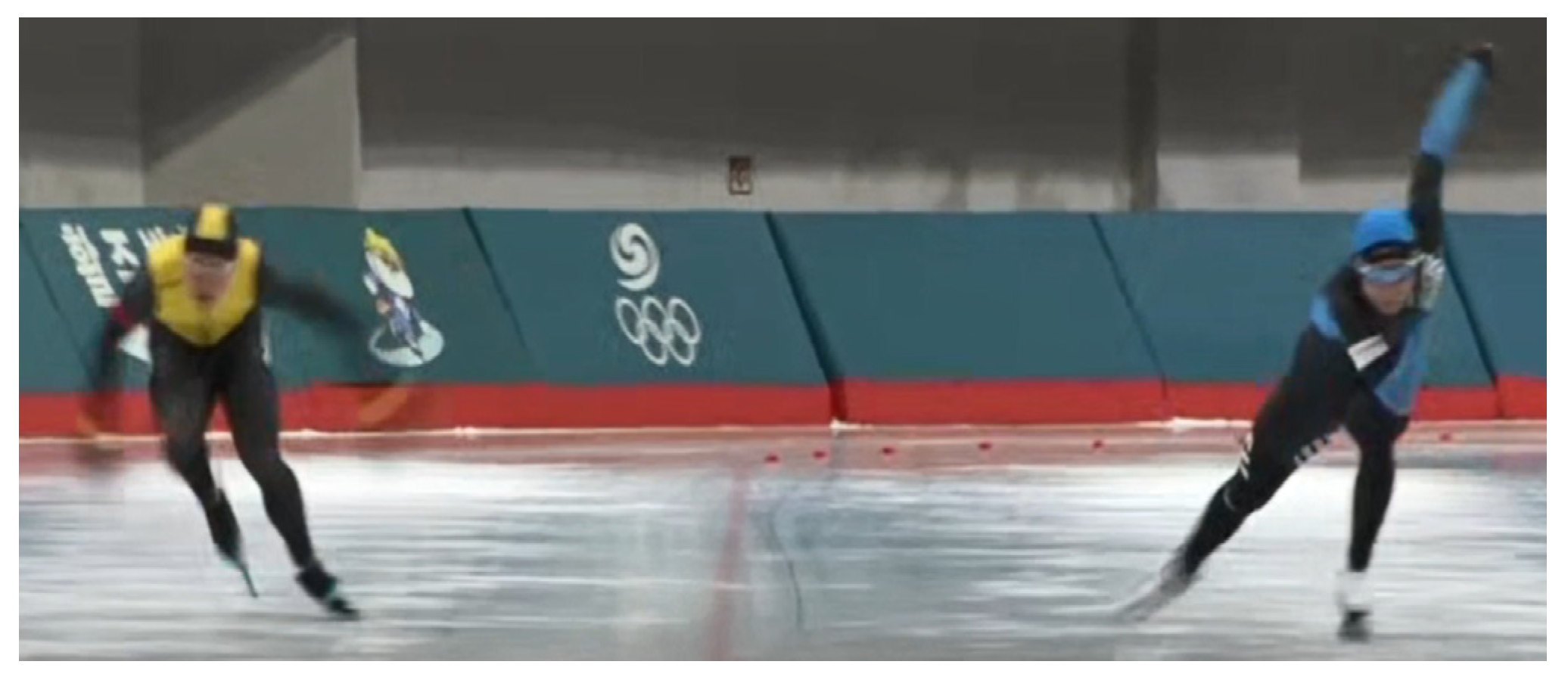
Because of the nature of speed skating, more than one athlete or individual can be displayed on a single screen. Figure 1 displays one such example. In these cases, the targets of landmark extraction are not fixed to a single person, and the coordinates of the landmarks are not reliable. Thus, ensuring the reliability of all steps after landmark extraction is difficult.
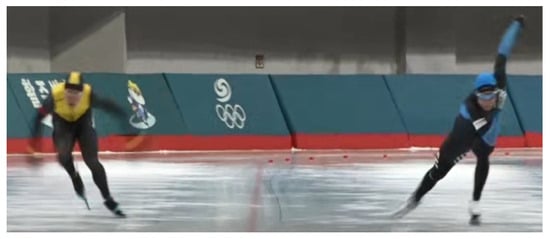
Figure 1.
Example with more than one person in a frame.
In addition, when users need to choose a performance measurement target, the system should incorporate a user-friendly process for target selection. Therefore, it is advantageous to explore methods that enable users to specify their desired measurement, addressing the concerns raised in the previous paragraph about accommodating multiple targets on a single screen.
The user inputs the region of interest (ROI) of the target in the first frame of the video as a bounding box using an input device such as a computer mouse. To ensure precise tracking with OpenCV’s tracker, users should choose only the head of the target as the bounding box. Including the entire body may lead to tracking issues stemming from factors like the background. The system then crops the image to an appropriate ratio to include the entire body of the subject, allowing for reliable stroke counting. By extracting landmarks from the cropped image, the user can ensure the accuracy of the measurement by fixing the target on a single person. This approach not only enables the sole use of the desired target for measurement but also ensures reliable results.
3.2. Joint Coordinate Extraction Using MediaPipe Pose
MediaPipe Pose provides the relative coordinates for 33 key body landmarks and can extract landmarks from images with partially occluded bodies. The process involves two steps: first, detecting the presence of a human via searching for the face and specifying the bounding box; and second, finding landmark points on the detected human. If detection fails in the first step, the process is repeated in the next frame.
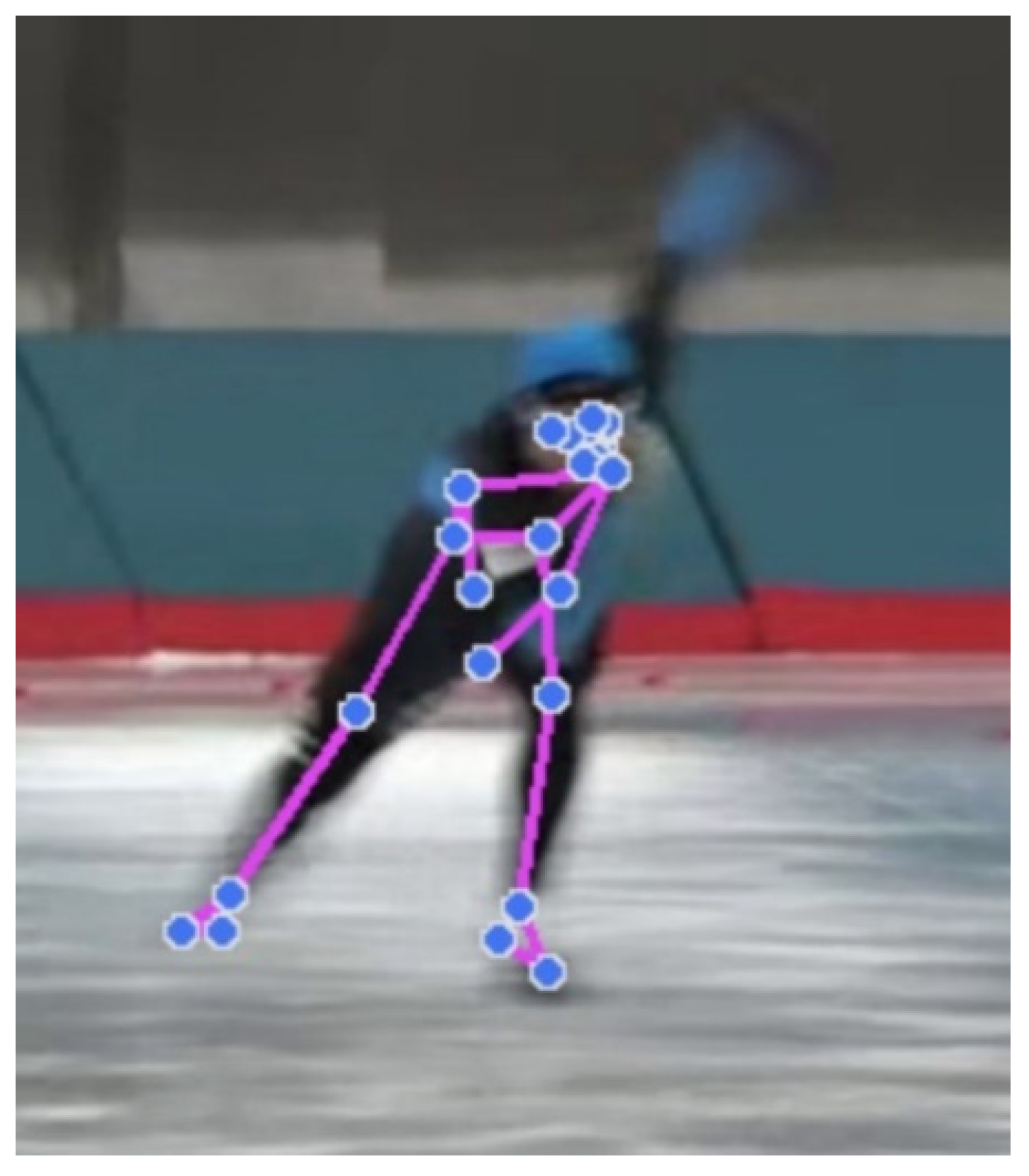
MediaPipe Pose is based on the work of Bazarevsky et al. on BlazePose [34], and has been shown to outperform the OpenPose model in terms of accuracy and FPS. Therefore, in this study, MediaPipe Pose is used to extract the coordinates of the main joint landmarks. Figure 2 illustrates the results of using MediaPipe Pose to extract the main joint (skeleton) landmarks in an athlete’s stroke motion.
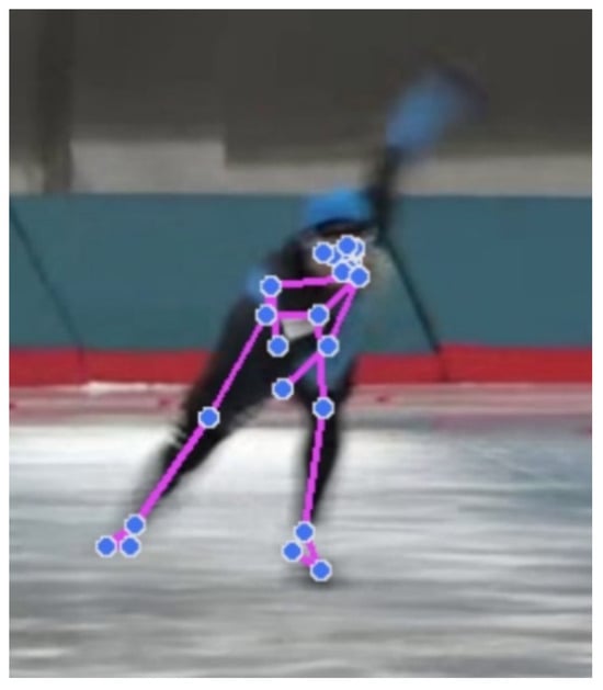
Figure 2.
Result of landmark points’ extraction. Each blue dot represents the landmark point of the target.
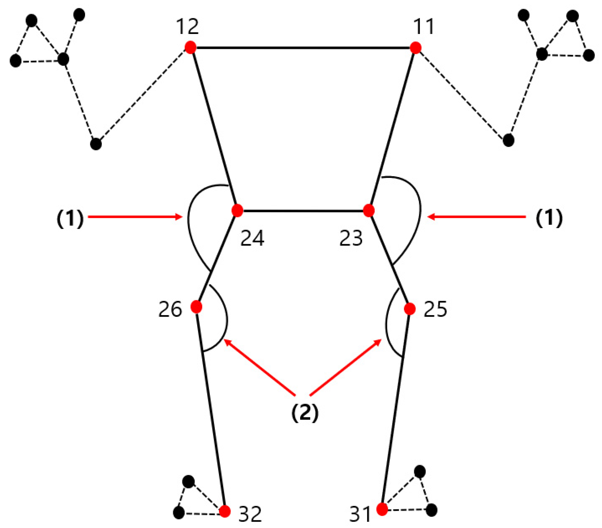
In the proposed method, MediaPipe Pose is used to extract the x-, y-, and z-coordinates of the subject’s body landmarks. From a subset of the 33 landmarks provided, 4 angles are calculated for each frame, in which each angle is a 3D angle between 3 points, using the x-, y-, and z-coordinates. Figure 3 displays the four angles used in this method, which correspond to specific articulation points on the body. The articulation point number is provided by MediaPipe Pose, and the following two types of angle, marked in Figure 3 as (1) and (2), are used in the system:
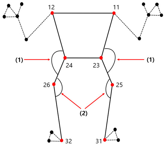
Figure 3.
Pelvic angles (1) and knee angles (2) at landmark points. Red dots represent landmark points used in this paper, and the numbers corresponding to the dots represent the number of each landmark point provided by Mediapipe Pose. (1) and (2) refer to the two types of body angles used in the algorithm of this paper.
- (1)
- Pelvic angle: the angle between the line starting at the shoulder (11, 12) and passing through the pelvis (23, 24) to the knee (25, 26).
- (2)
- Knee angle: the angle between the line starting at the pelvis (23, 24) and passing through the knee (25, 26) to the ankle (31, 32).
All angles are expressed using smaller angles that do not exceed 180° based on the sexagesimal system.
3.3. Joint Coordinate Tracking Using OpenCV
OpenCV is a library developed for machine learning, image processing, and computer vision. OpenCV supports operations using various programming languages and operating systems. OpenCV provides a tracker function based on various algorithms for tracking moving objects. The system in this study utilizes the CSRT [35] tracker for tracking the moving players, which exhibits relatively stable tracking performance in various environments.
OpenCV’s CSRT Tracker utilizes the CSR-DCF method proposed in Lukezic et al.’s paper [36]. CSR-DCF is an extension of the DCF tracking algorithm. The correlation filter is updated to track the target using two feature points, histograms of oriented gradients (HoGs), and color names. An object can be tracked even if it is not rectangular. In many cases, the object to be tracked in the system used in this study was difficult to define in a clear rectangular shape; therefore, the CSRT tracker was used to track the object.
In every frame, the head of the object to be measured is tracked based on the bounding box initially input by the user. Based on the tracked head, the top, bottom, left, and right sides are cropped in an appropriate ratio. By repeating the process of taking the cropped image as the input for skeleton extraction, the key joint coordinates can be extracted from all video frames.
3.4. Angle Calculation
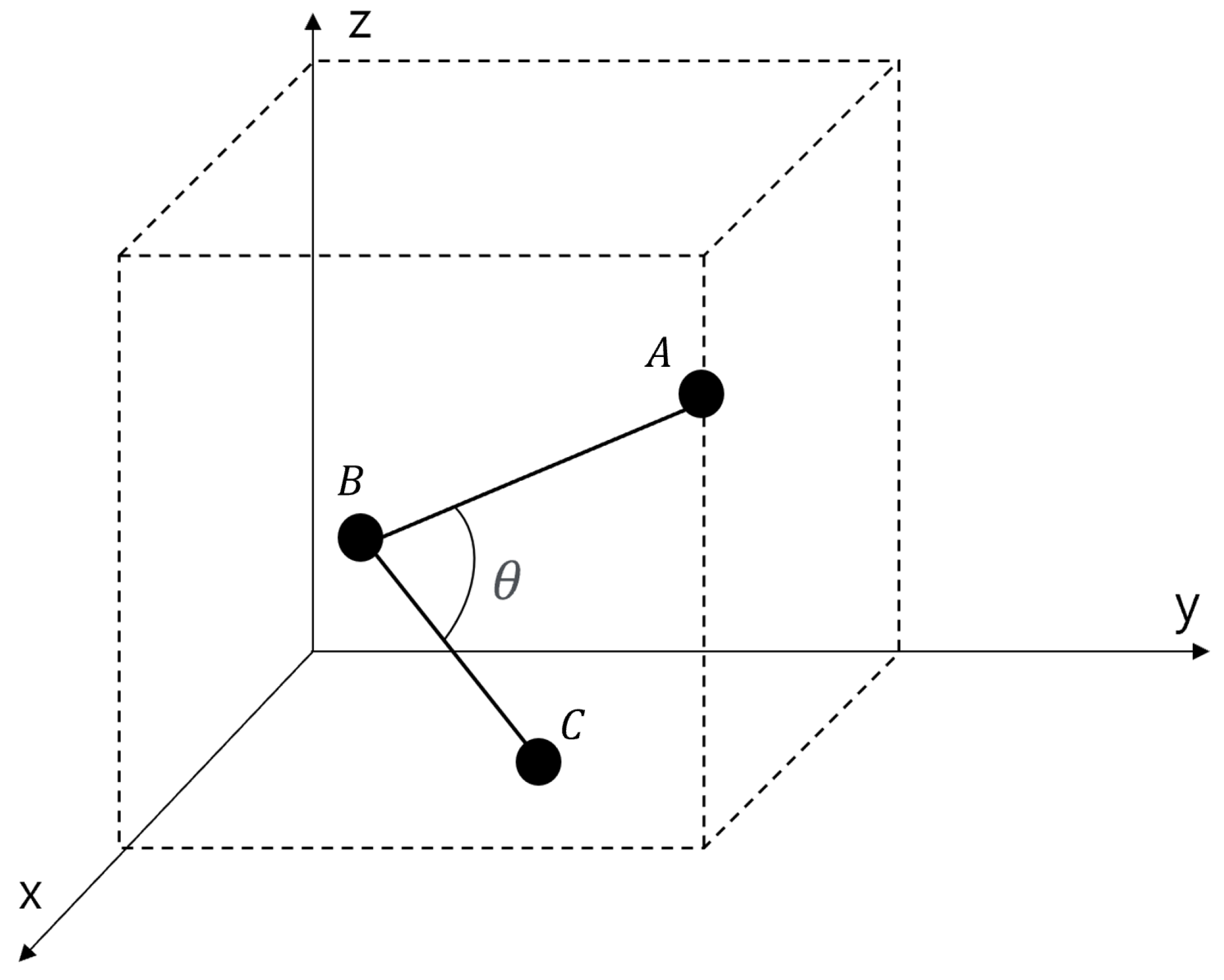
This section describes the calculation of the four angles, namely the knee and pelvic angles, that will be utilized in the proposed system. As mentioned, the coordinates of the landmarks provided by MediaPipe Pose represent the coordinates in a three-dimensional space. The three points used for calculating the angles are denoted as and , with the angle being represented by the angle that needs to be determined. The relationship between the three points and can be observed in Figure 4.
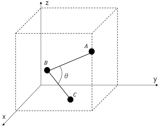
Figure 4.
Relationship between and .
Angle can be determined using the definition of the dot product of vectors. According to the definition of the vector dot product, an arrangement as shown in Equation (1) can obtained, and can be determined using Equation (2). As mentioned, the four angles to be used after landmark extraction use a smaller angle that does not exceed 180° based on the sexagesimal system. Therefore, if an angle of 180° or greater is extracted after calculating the angle, the value subtracted from 360° is used.
3.5. Analyzing Angles Based on Stroke Motions
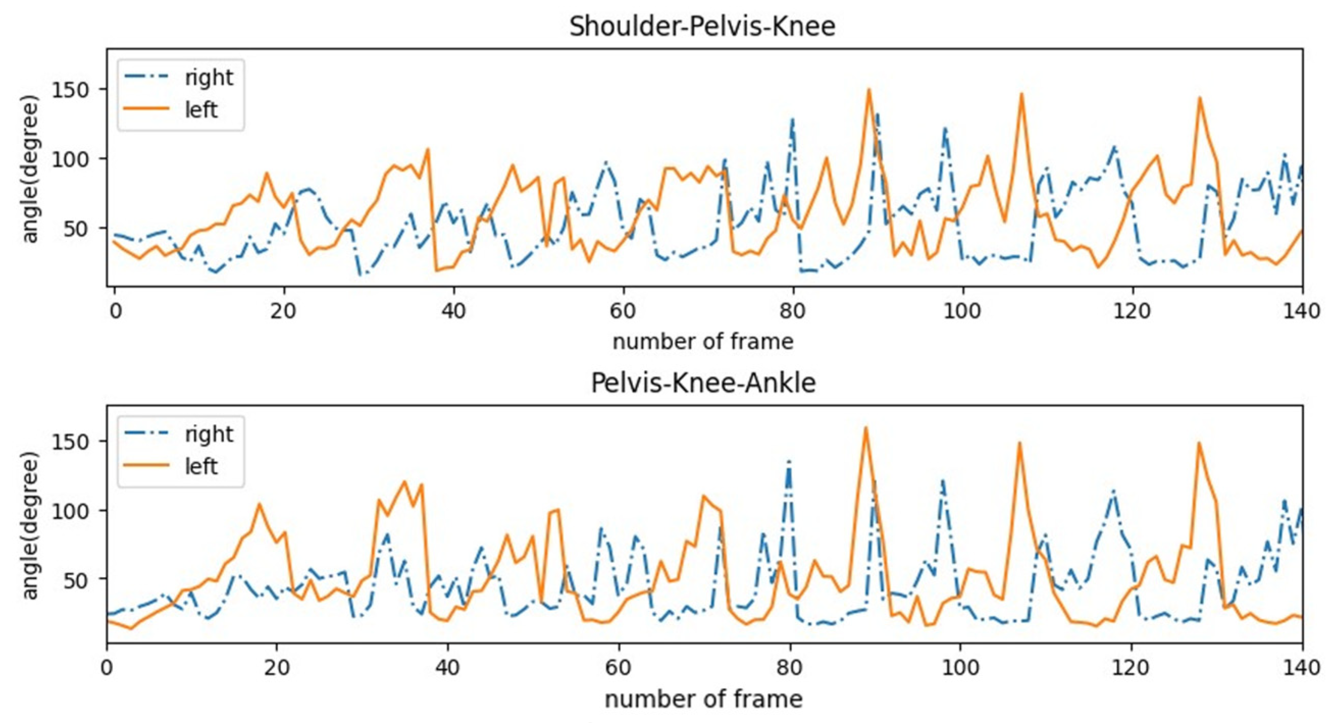
The distinction between the left and right strokes in the stroke motion is clear. Because measuring the number of stroke movements is equivalent to measuring the number of times an athlete moves their body from side to side, a system that takes advantage of this characteristic may be designed. Comparing left and right stroke motions reveals an evident inverse relationship between the two angles derived from each side of the body. Specifically, the angle extracted from the left side of the body decreases when the measured object strokes to the left (from the perspective of the measured object), whereas the angle extracted from the right side increases. This difference is clearly visible when the corresponding angles are extracted and compared across a series of strokes, as displayed in Figure 5. Figure 5 details a comparison of the angles up to approximately 140 frames after the start of measurement. The video used for the comparison was recorded at 30 frames per second.
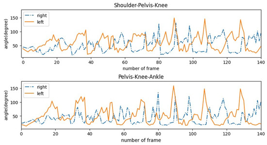
Figure 5.
Comparison of left and right pelvic angles (top) and left and right knee angles (bottom).
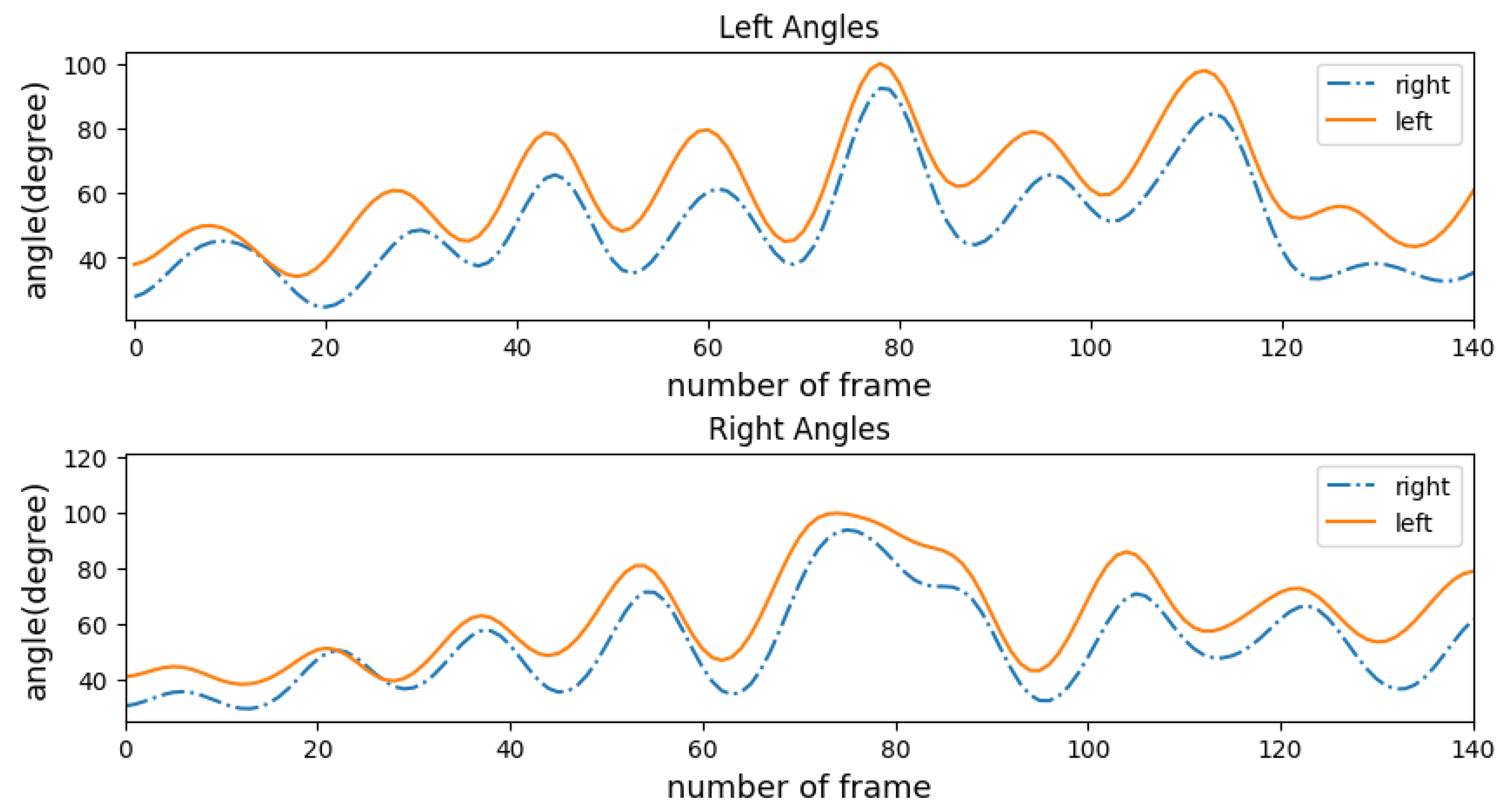
All four angles are utilized to quantify the strokes, aimed to establish the vertical relationship between the angles extracted from the left and right sides of the body. To ensure the system’s accuracy, it is necessary to examine whether the angles taken from the left and right exhibit the same tendencies. If the two angles obtained from the left have distinct tendencies, only one angle from each side may be used to measure the number of strokes. Figure 6 shows the results of comparing the values of the left and right knee angle and pelvic angle on a frame-by-frame basis. As a result, we can see that both types of angles show the same tendency on the left and right.
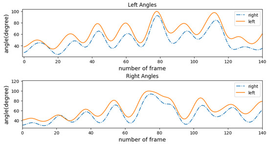
Figure 6.
Confirmation of left–right angle relationships.
In the stroke images, the angle change in the arm according to the left and right stroke motions is more observable than that in the pelvis and knee. Therefore, angles that can be extracted from the upper extremities, that is, from the shoulder to the wrist, can be used to distinguish between stroke motions more clearly. Due to the rapid arm movements in speed skating, especially in comparison to the rest of the body, tracking the upper extremities in each frame at a 30 frames-per-second rate is frequently unfeasible due to motion blur. Figure 7 depicts an example of a frame in which the clear position of the upper extremities is difficult to determine because of motion blur.
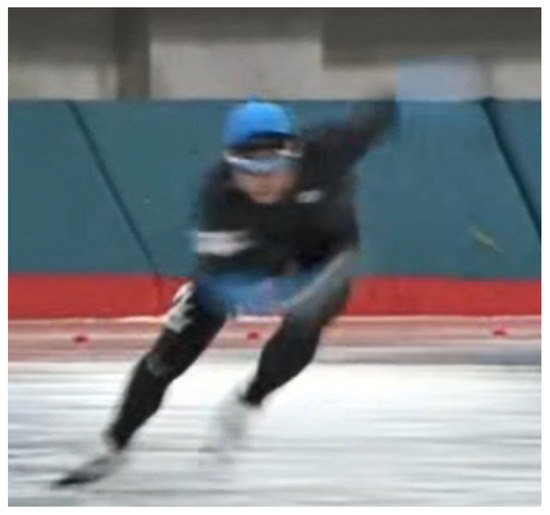
Figure 7.
Example of an arm afterimage.
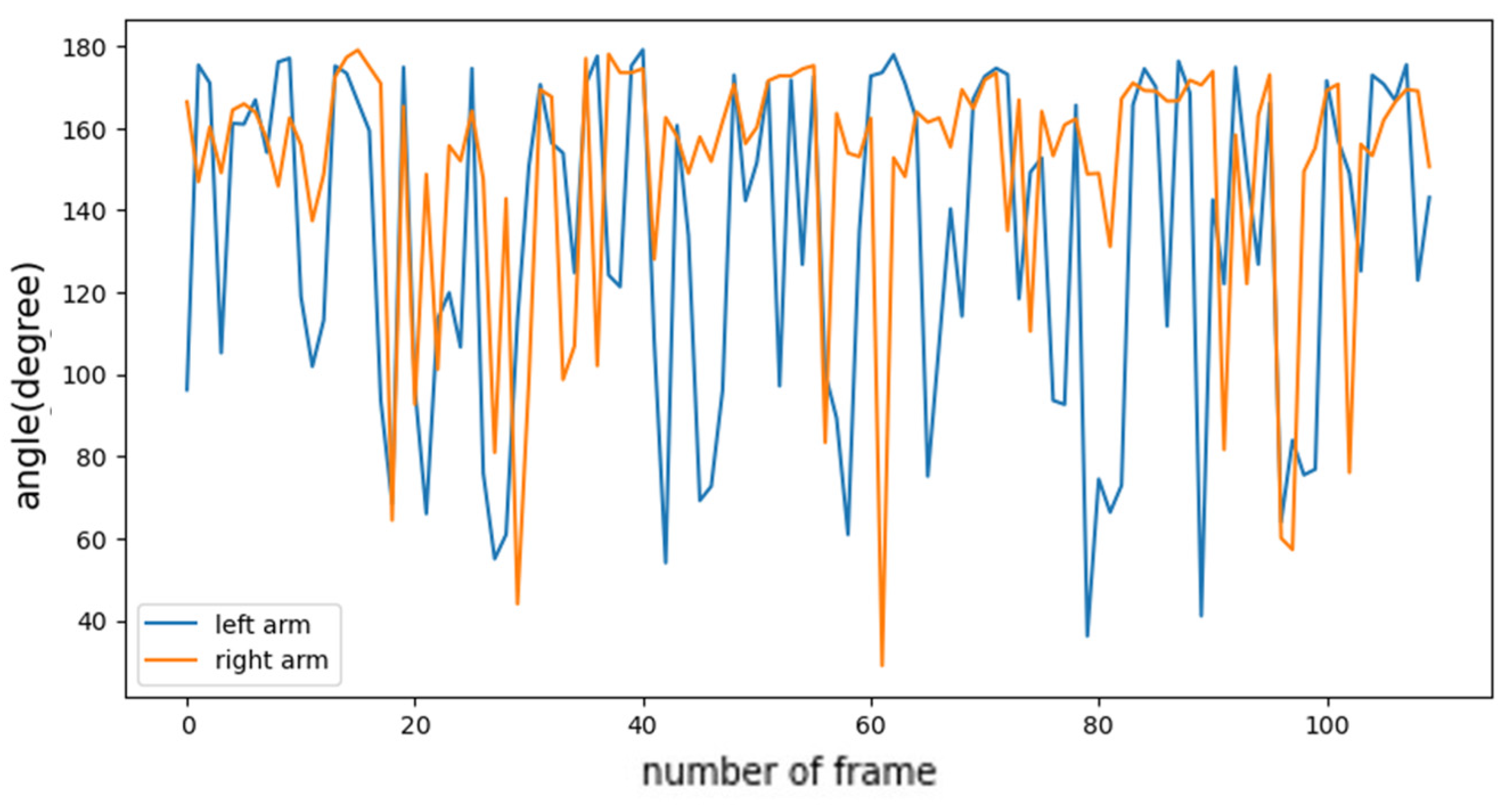
When the left and right arm angles from the shoulder to the wrist are measured and arranged by frame sequence, a graph is observed, as shown in Figure 8. Unlike in Figure 5, no clear trend is observed. This indicates that the process following landmark coordinate extraction may not be reliable; therefore, arm movements are not used in stroke counting. Instead, the focus is on body parts from the shoulder to the pelvis and ankles, which produce fewer afterimages owing to less vigorous movements.
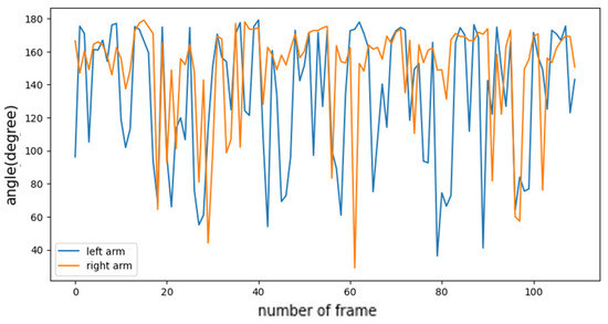
Figure 8.
Left and right arm angles.
3.6. Generalized Labeling Logic
The GLL (generalized labeling logic) index is established based on the calculation of four angles for each frame. Equation (3) defines the GLL by utilizing the properties of these angles. Confirming the GLL, it provides criteria for differentiating left and right stroke movements. In accordance with the camera viewpoint, the defined GLL diminishes when the stroke motion of the target shifts left and increases when it shifts right. Figure 9 effectively demonstrates this trend, presenting GLL measurements and distinguishing left and right strokes by segmenting them based on the camera’s frame unit.
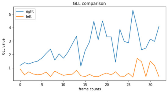
Figure 9.
Direct comparison of left and right stroke motions using GLL.
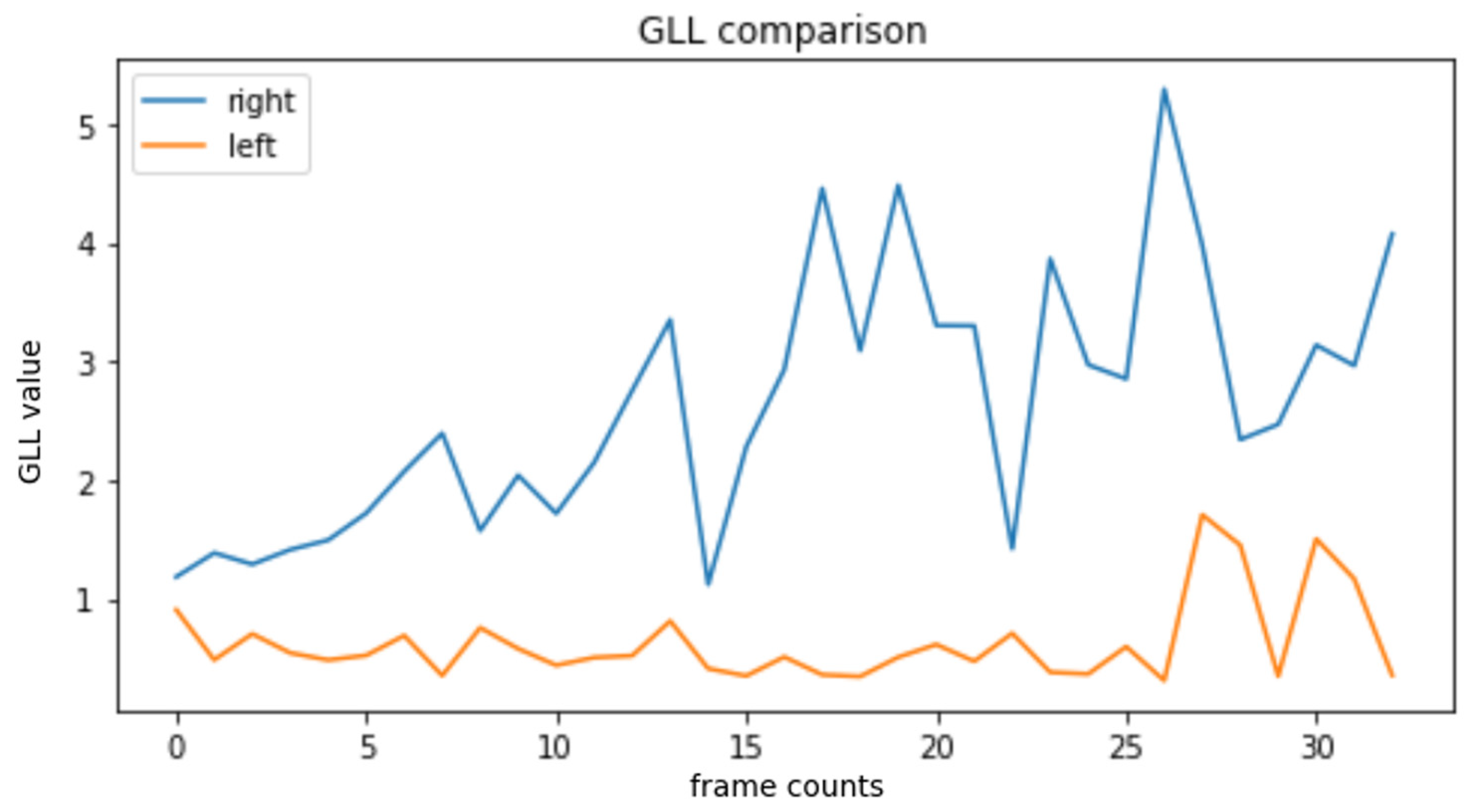
This comparison confirms that the GLL in the left and right stroke motions shows a difference in scale. From the results in Figure 10, it can be inferred that, when the GLLs are arranged in the frame order of the video, the signal increases in the right stroke and decreases in the left stroke.

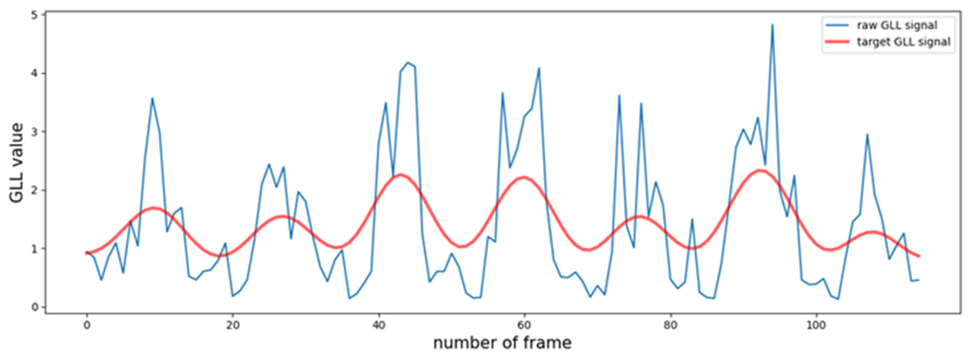
Figure 10.
Example of the raw GLL signal and target GLL signal. Since there is more noise in the raw GLL signal than the target, a noise-removal process is necessary.
The automatic stroke measurement system calculates the GLL for each frame and stores it in a list in frame order. After the GLLs for all video frames are stored, the list of stored GLLs is regarded as a single signal whose frame number is the time axis. Figure 10 displays a portion of the original GLL signal (up to 115 frames after stroke start) extracted from the actual stroke video and the ideal target GLL signal for counting the number of strokes.
The extracted signal indicates that the left and right stroke motions can be distinguished. In the signal, each wave cycle corresponds to the left and right stroke movements of the measurement target. The stroke count can be determined by counting the number of wave cycles within the GLL signal. However, compared to the target GLL signal, the raw GLL signal has noise. This occurs when the GLL signal is not a fluctuation caused by a stroke alone. This noise acts as an unnecessary factor in measuring the final stroke count. Therefore, it is critical to remove the noise from the raw GLL signal.
3.7. Filtering Signal
The characteristics of the signal to be extracted by filtering the GLL signal are defined as follows:
- Characteristic 1: Identify one frame that corresponds to the inflection point in each cycle.
- Characteristic 2: Remove any noise present in the original signal other than the cycles from the stroke.
- Characteristic 3: Remove cycles from strokes simultaneously during the denoising process or generate no additional cycles.
Characteristics 1 and 2 ensure measurement accuracy. If one or more vertices can be identified from the cycle generated by each stroke movement, establishing clear criteria for processing each inflection point in the filtered GLL signal becomes difficult. This result can be a problem in terms of the accuracy of the system; therefore, the post-filtering signal should satisfy both Characteristics 1 and 2. Characteristic 3 is also intended to ensure the accuracy of the results. Applying strong filtering to remove noise can remove cycles generated by stroke movement, which renders measurement results unreliable. However, if additional cycles are generated, the measured results may exceed the actual stroke count. Therefore, ensuring that such problems do not occur in the post-filtering signal is critical. If we can obtain a noise-free GLL signal that satisfies all three characteristics, the stroke count can be obtained by simply counting the number of vertices in the signal.
In this study, two signal-filtering methods are considered: Gaussian filtering and fast Fourier transform (FFT)-based high-frequency component removal. Each method has been evaluated to determine the effectiveness of noise removal from the GLL signal, and the more appropriate method was selected for this study.
3.7.1. FFT-Based Filtering
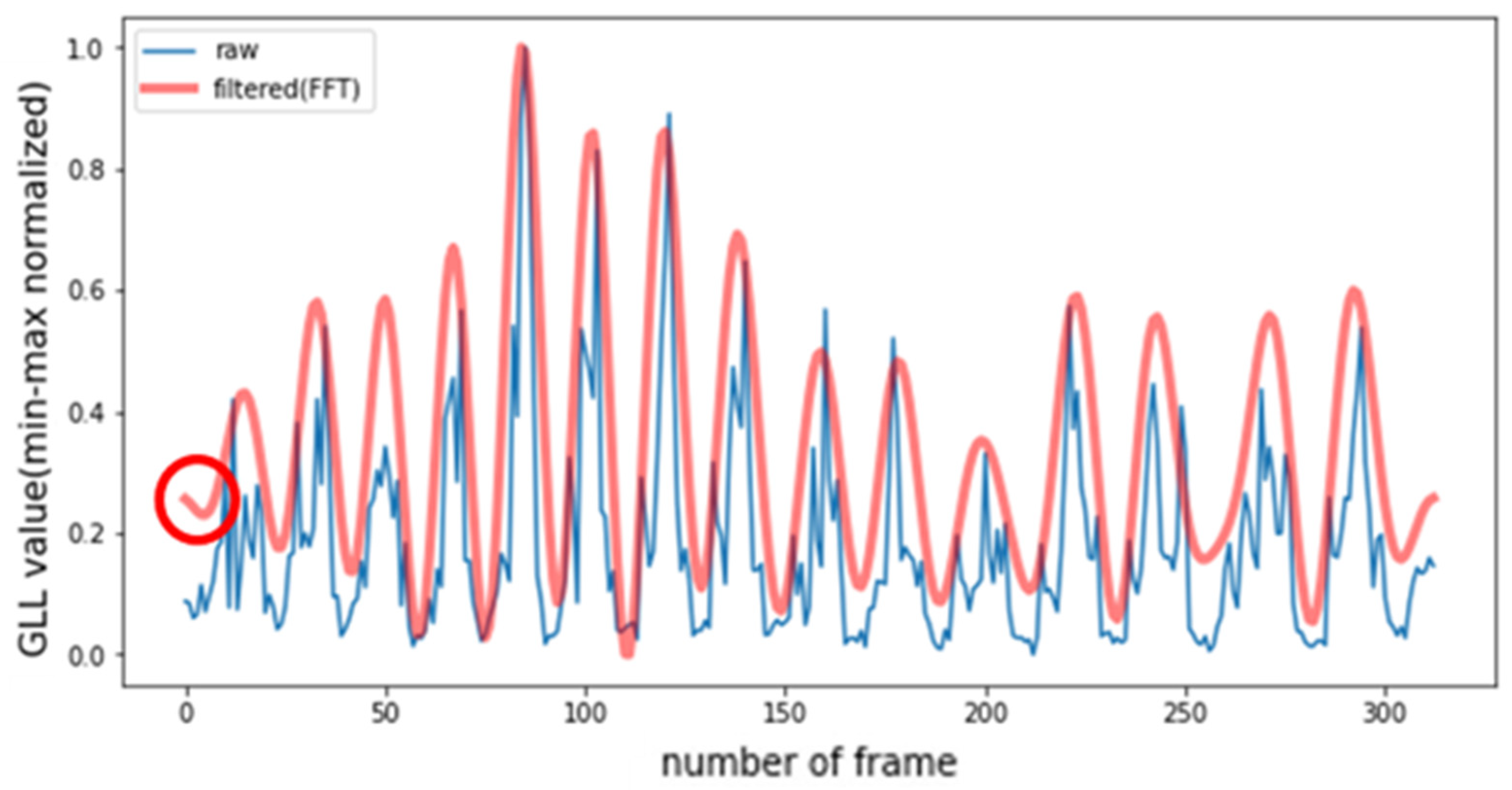
FFT is an algorithm that is designed to rapidly calculate the DFT, and a signal in the time domain can be transformed into the frequency domain [37]. FFT also allows for inverse operations, enabling the transformation of signals from the frequency domain back to the time domain for analysis. Assuming that the noise of the GLL signal is caused by the signal in the high-frequency domain, a possible method for reducing the noise is to first convert the signal to the frequency domain using FFT. Subsequently, the high-frequency component can be identified and removed from the signal. Finally, the signal can be restored to its original form by performing the inverse FFT operation on the modified signal. The signal recovered in this manner is the signal from which high-frequency components, e.g., noise, have been removed from the original GLL signal. Figure 11 displays the result of noise removal using the method through a comparison with the original signal. Min–max normalization was performed on both the original and filtered signals to compare the two signals. This normalization process only clarifies the comparison between the original signal and the signal after filtering. Therefore, the process is not included in this study’s stroke-measurement process.

Figure 11.
FFT-based filtering results. The point indicated by the red circle indicates the point where an unintended additional wave occurred during the filtering process.
At the start of the stroke motion, the filtering of results encounters a problem. As displayed in Figure 11, an additional cycle exists at the start of the filtered signal that is not visible in the original GLL signal. This cycle does not satisfy Characteristic 3 of the filtered-signal conditions described earlier. This problem cannot be solved by adjusting the filtering frequency range or image selection. Because of these problems, a filtering method that limits the frequency range is not used.
3.7.2. Gaussian Filtering
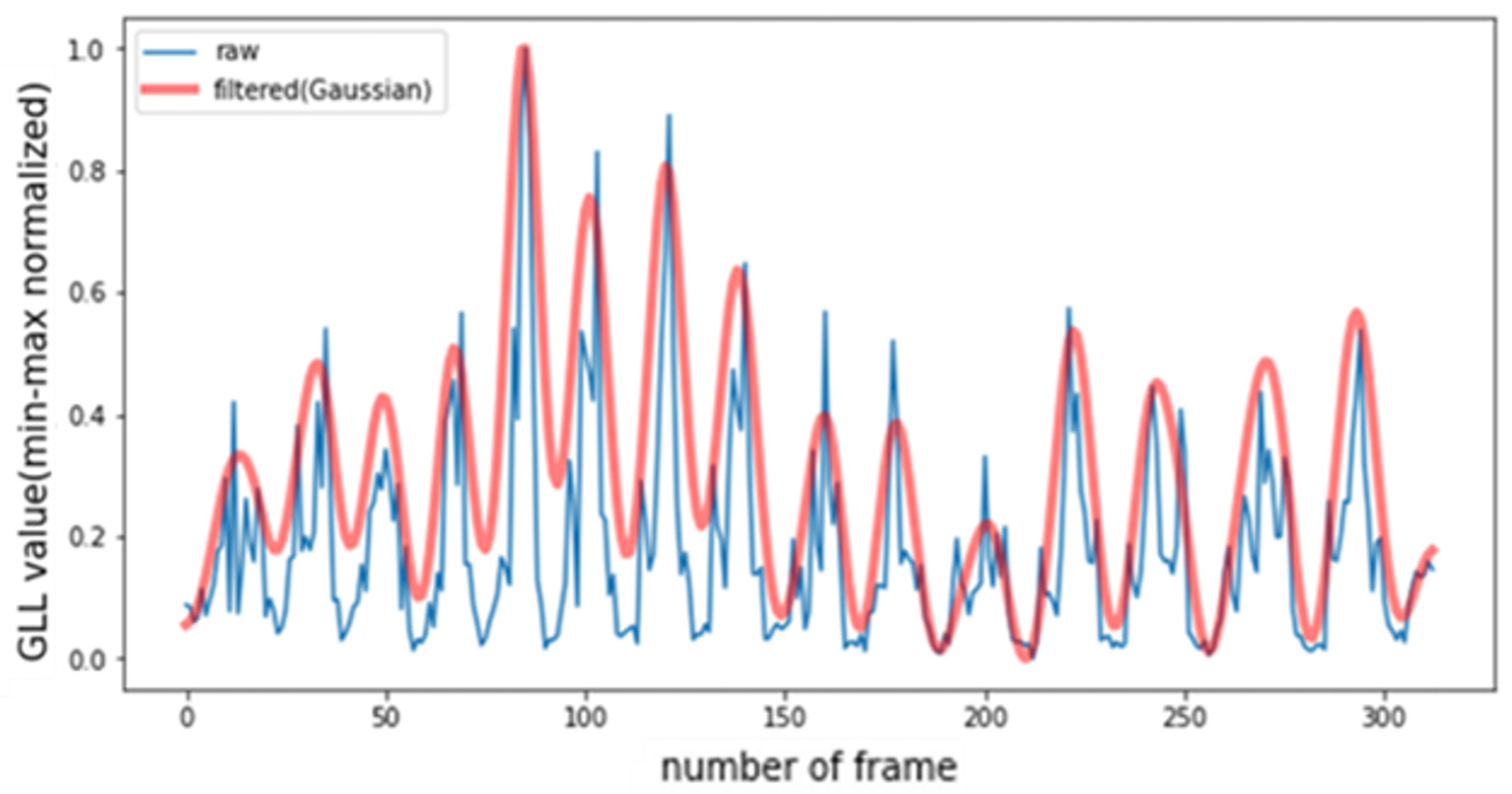
Gaussian filtering refers to filtering based on a Gaussian distribution. Figure 12 displays the result of denoising the original GLL signal with Gaussian filtering and comparing it with the raw signal. For a clear comparison, both the original and filtered GLL signals have been min–max normalized; the normalization process continues not to be included in the stroke-measurement process of the final system.
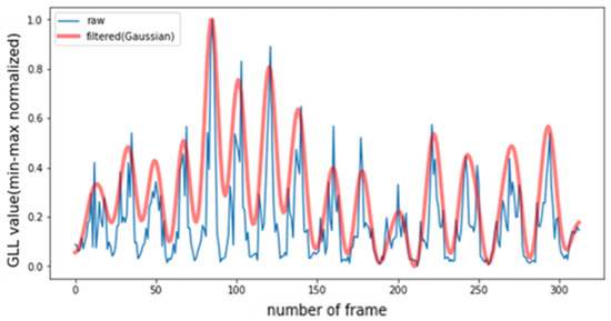
Figure 12.
Gaussian filtering results.
Because of the filtering, the problem of generating additional cycles, which was confirmed in the FFT-based filtering result in Figure 11, is not observed. As displayed in Figure 12, a filtered GLL signal that satisfies Characteristics 1, 2, and 3, defined above, can be obtained when an appropriate sigma value is provided. Thus, Gaussian filtering can effectively remove noise from the original GLL signal if an appropriate sigma value is provided. Based on these characteristics, a Gaussian filter is used to filter the GLL signal in the proposed stroke number measurement system. In this process, the sigma value of the Gaussian filter proposed in this study is 3.4. Figure 13 displays the final GLL signal with noise removed using a Gaussian filter.
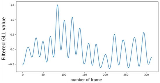
Figure 13.
Final GLL signal with noise removed.
An approach was considered on how to filter the signal using Gaussian filtering following FFT-based filtering, which exhibits excellent performance. This result was not considered as there was no noticeable performance difference compared to only using Gaussian filtering. Additionally, adding an extra filtering process is unnecessary when the performance difference from Gaussian filtering is not evident.
3.8. Stroke Count
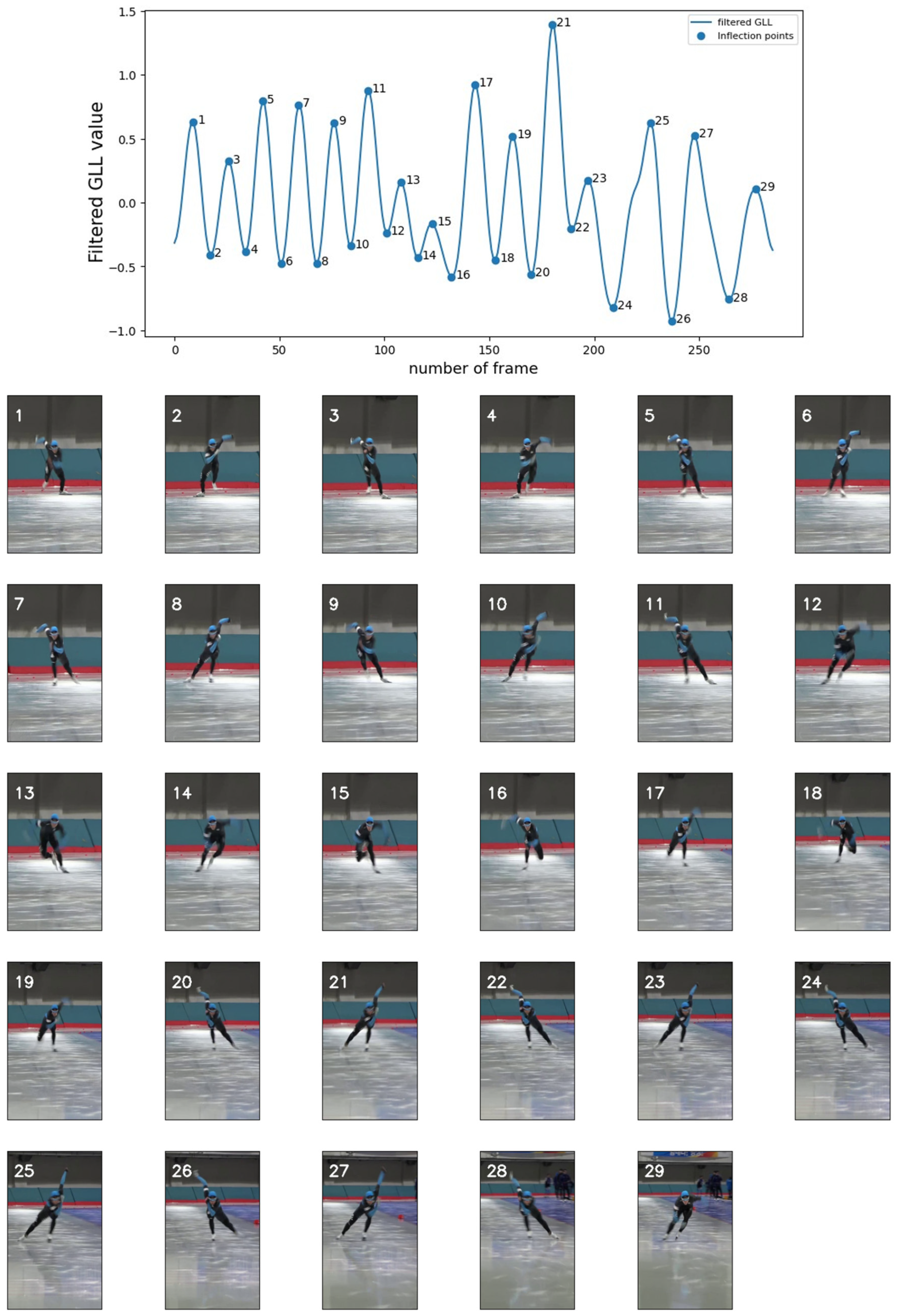
In relation to the stroke count, the GLL signal for all frames was obtained by calculating the GLL for each frame, with the noise being removed from the original GLL signal through Gaussian filtering. Finally, the stroke number measurement system was designed by determining the method for extracting the stroke number from the filtered GLL signal. As displayed in Figure 13, the GLL signal after filtering takes the form of a cycle that oscillates at regular intervals. Each waveform of the cycle is based on the classification of left and right stroke motions according to the properties of the GLL index. Therefore, the number of strokes can be measured by counting the number of cycles in the entire filtered GLL signal. The proposed system makes this possible by counting the number of vertices in the filtered GLL signal. Figure 14 details an example of the number of final strokes measured using this method and the corresponding frames.
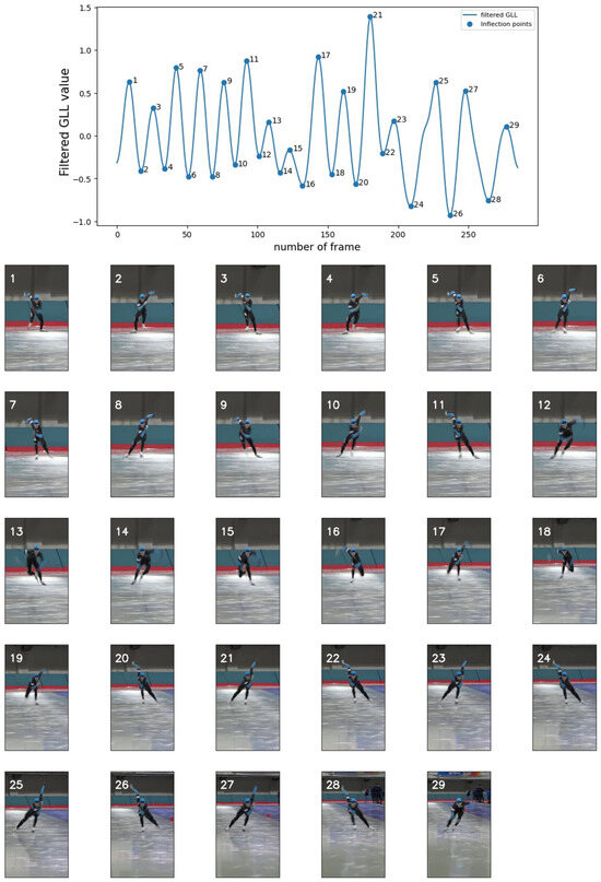
Figure 14.
Stroke count measurement results (top) and corresponding frames from video (bottom). Each image is associated with the stroke inflection point number on the graph above. Each frame represents the corresponding frame in the video when each inflection point occurred.
3.9. Final System Description
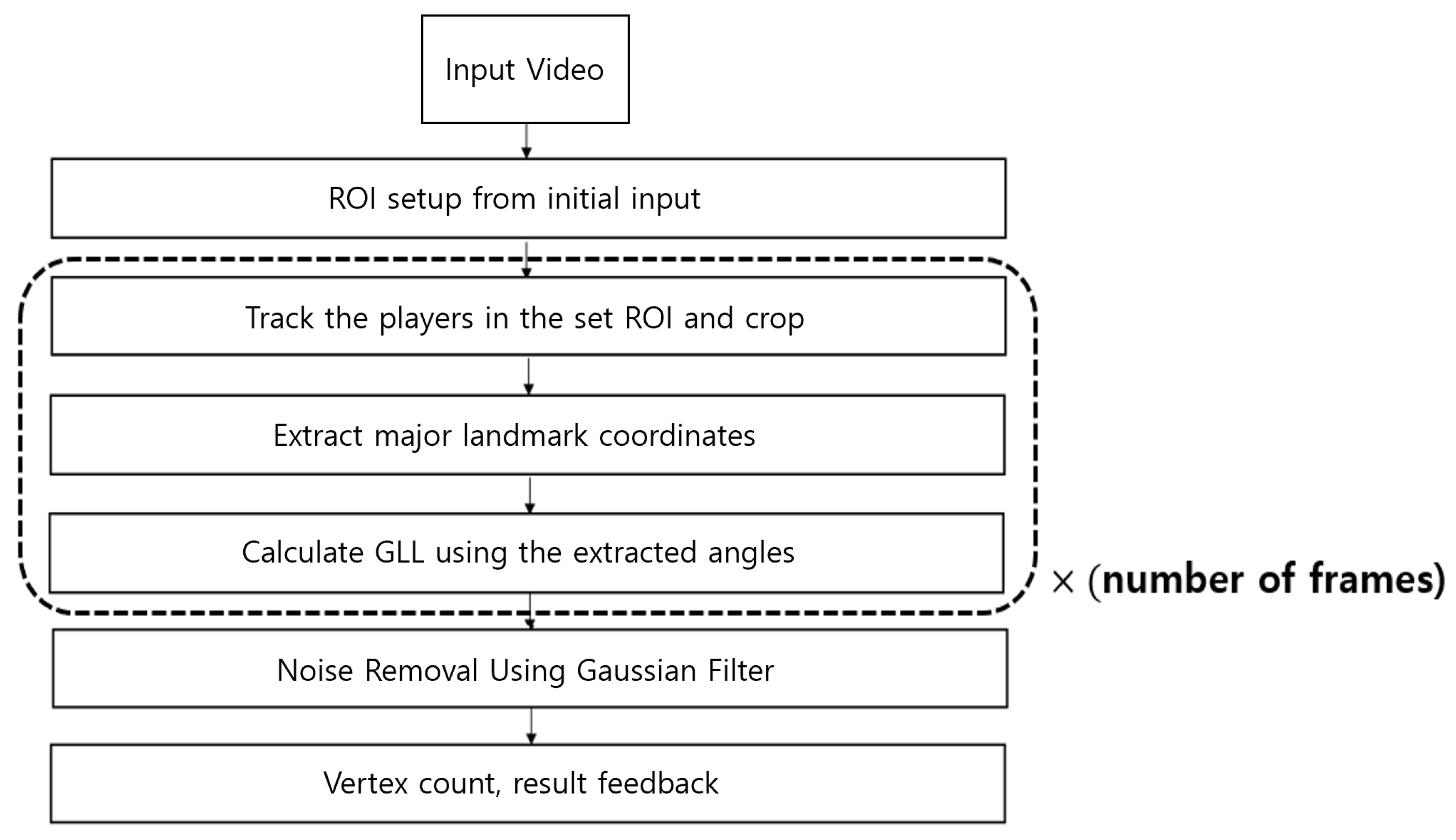
Figure 15 displays the schematic of the proposed speed skating stroke-counting system. In this system, a video of the first 100 m is prepared after departure which contains the subject to be measured. Subsequently, the system requests that the user input the ROI of the subject to be used for tracking in the form of a bounding box through an input device such as a computer mouse. At this time, the “subject” is the player or individual whose stroke count is to be measured. Subsequently, using the OpenCV tracker, the object entered by the user is tracked for each frame, and the image is cropped such that only the object to be measured remains. The landmark x-, y-, and z-coordinates of the target are extracted from the cropped image using MediaPipe Pose. The extracted 3D coordinates are used to calculate the body angles required for stroke count measurements (pelvic and knee angles). By using these angles, the GLL is calculated and stored in the frames. This operation is repeated for all frames of the user’s video input, resulting in a GLL list. Once the GLL list is generated by repeating the above process for all frames of the user’s video input, noise is eliminated using Gaussian filtering. In this process, each GLL value in the list is treated as a continuous signal with the frame number as the time axis. The stroke count system is completed by counting the number of vertices in the noise-free signal and feeding it to the user.
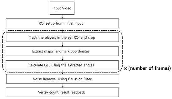
Figure 15.
Automatic stroke count system.
4. Experiment Results
In this section, examples of the system’s results will be shown, focusing on frontal videos. Afterwards, the results of experiments conducted on both frontal videos and side videos will be presented. Lastly, actual usage screens will be illustrated and will show how the system presented in this paper can be used in practice.
The experiments are categorized into two types of videos: videos captured from the front and videos captured from the side. In the process of designing the system, side videos were not considered; however, experiments were conducted to check whether the system designed in this study was versatile enough for videos from various angles.
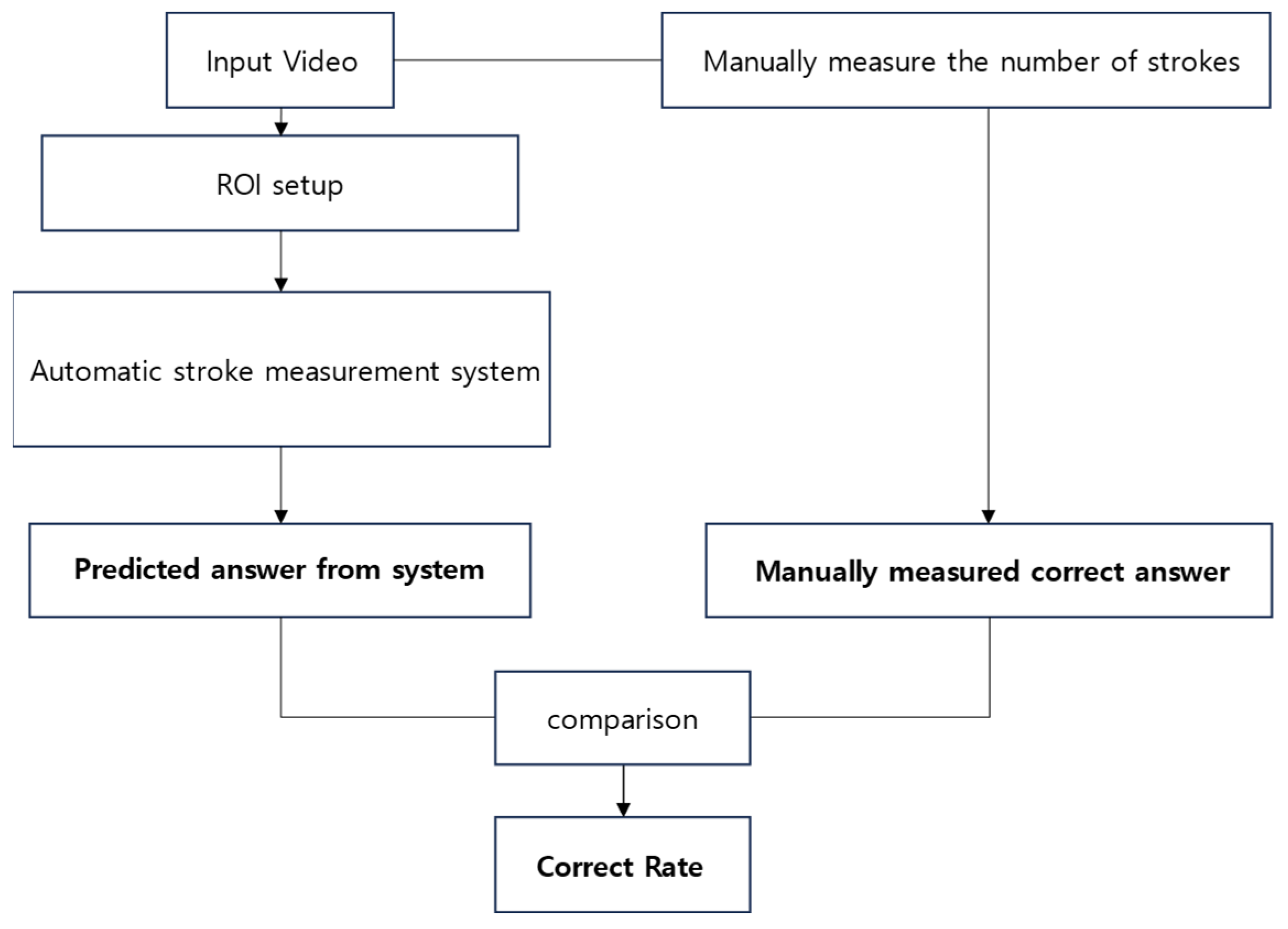
For the frontal videos, videos of the first 100 m of the straightaway after the start of four speed skaters were used. Each skater’s actual number of strokes was manually measured and the correct answer was obtained. Subsequently, considering that the results may vary depending on the state of the user’s bounding box input, the bounding box was freshly applied 10 times per skater, measured using the proposed method, and compared with the correct answer. Figure 16 shows the overall sequences that were conducted in the experiment. The experiment sequence shown in Figure 16 was the same in both the frontal and side videos.
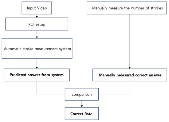
Figure 16.
Overall sequence of the experiment. This sequence was conducted in the same way in both frontal and side videos.
Figure 17 shows an example of side-view video frames. Figure 18, Figure 19, Figure 20, Figure 21 and Figure 22 illustrate the actual bounding box input and stroke count measurement results for the videos of Players 1, 3, and 4. In particular, Figure 21 and Figure 22 demonstrate a comparison of the bounding box input and measurement results for Player 2, the only measurement subject that caused an error in the experimental results. Figure 21 displays the result of the correct case, and Figure 22 shows the result of the round in which the error occurred.
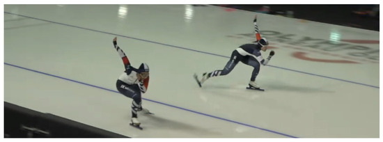
Figure 17.
Example of side-view video frames. In this experiment, the same method was applied to the side-view video as for the frontal video.
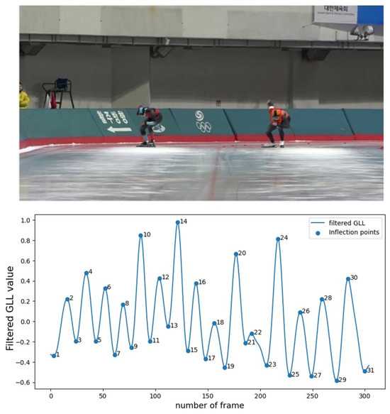
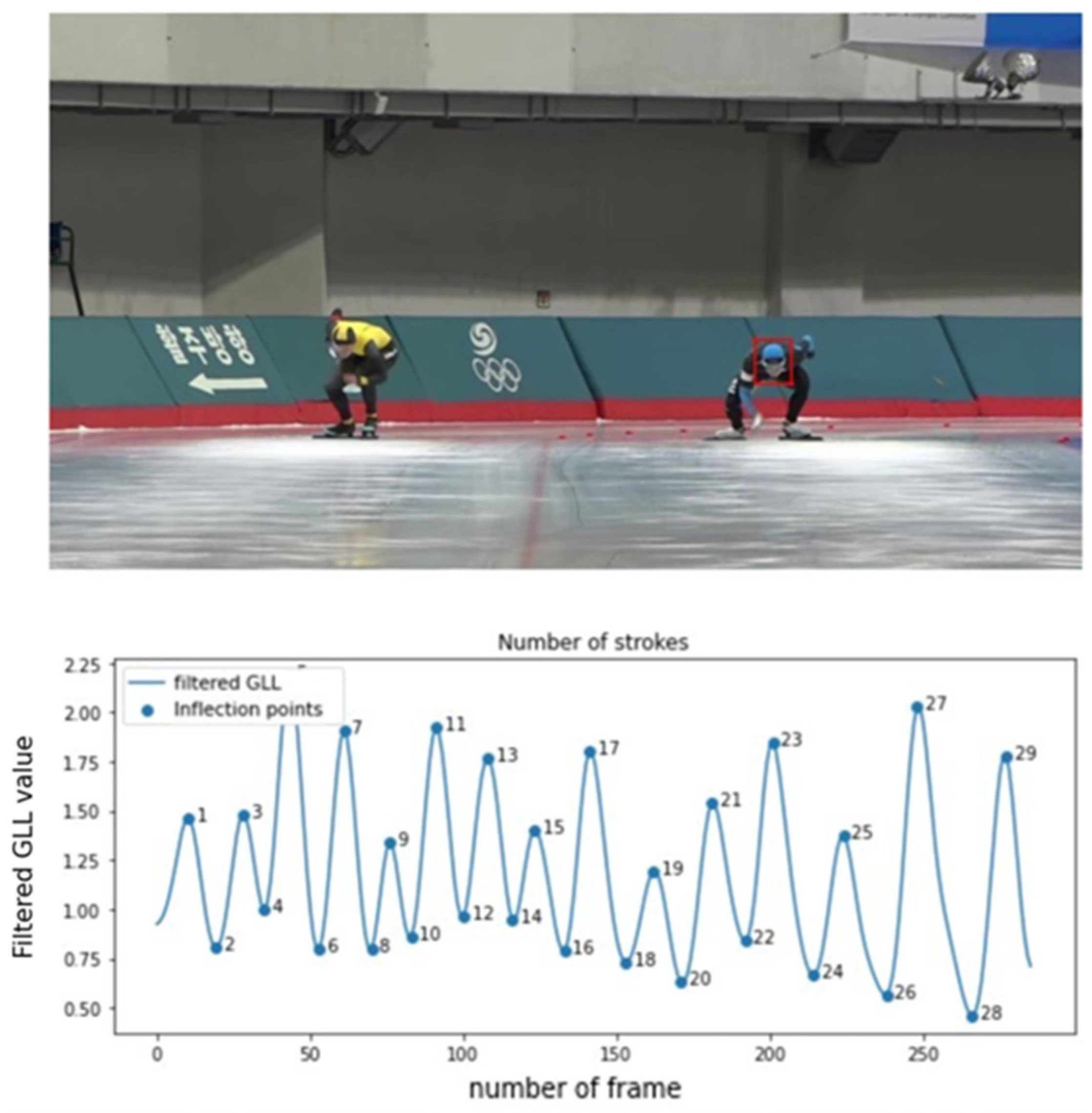
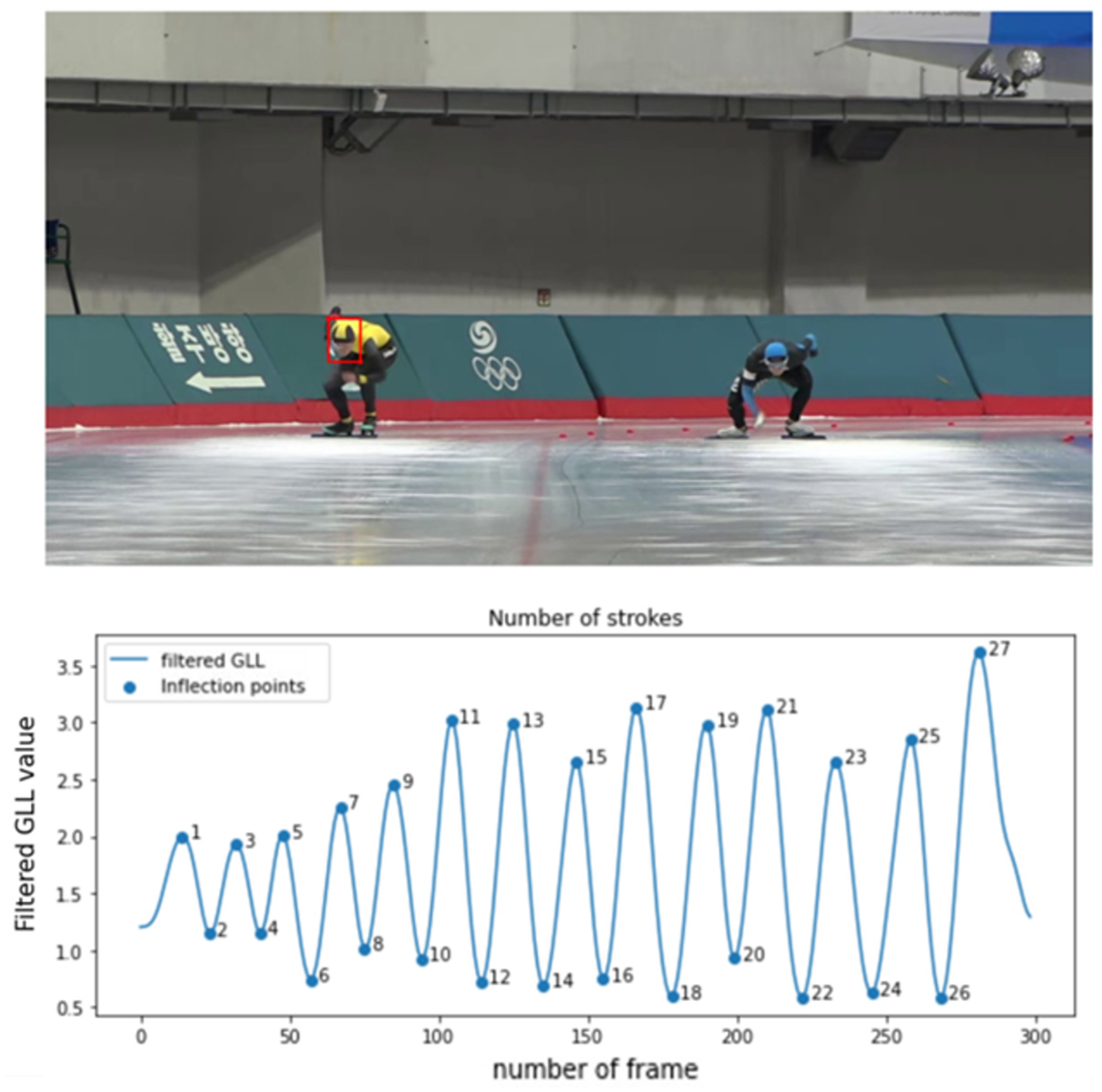
Figure 18.
Player 1: experimental results. A bounding box drawn around Player 1’s face (top) and inflection point positions extracted from the GLL signal obtained from Player 1 and the stroke count at each of these positions (bottom). In the top image, the video of the player on the right side of the screen is used.

Figure 19.
Player 3: experimental results. A bounding box drawn around Player 3’s face (top) and inflection point positions extracted from the GLL signal obtained from Player 3 and the stroke count at each of these positions (bottom). As can be seen in the top image, the video of the player on the right side of the screen is used.
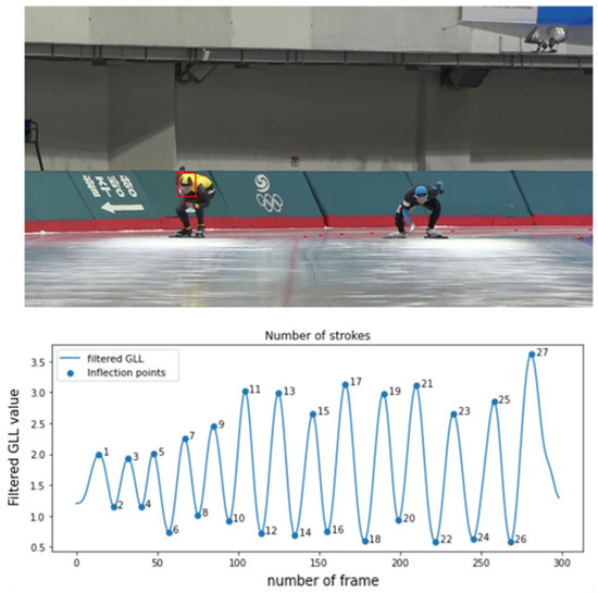
Figure 20.
Player 4: experimental results. A bounding box drawn around Player 4’s face (top) and inflection point positions extracted from the GLL signal obtained from Player 4 and the stroke count at each of these positions (bottom). As can be seen in the top image, the video of the player on the left side of the screen is used.
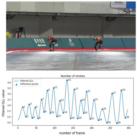
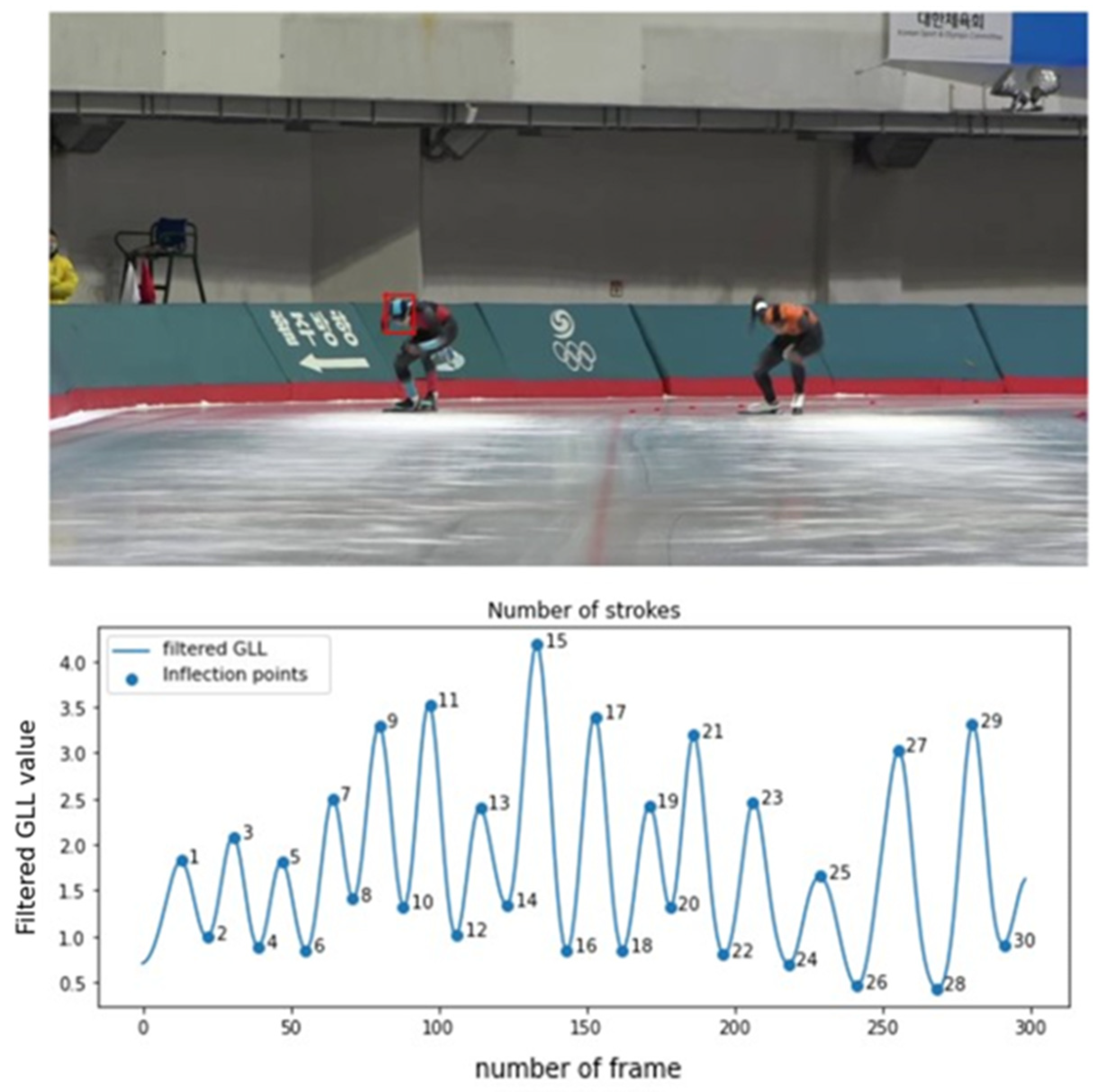
Figure 21.
Player 2: experimental results. A bounding box drawn around Player 2’s face (top) and inflection point positions extracted from the GLL signal obtained from Player 2 and the stroke count at each of these positions (bottom). As can be seen in the top image, the video of the player on the left side of the screen is used. This figure addresses the case where Player 2’s stroke counts match the correct answers.
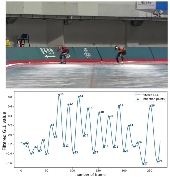
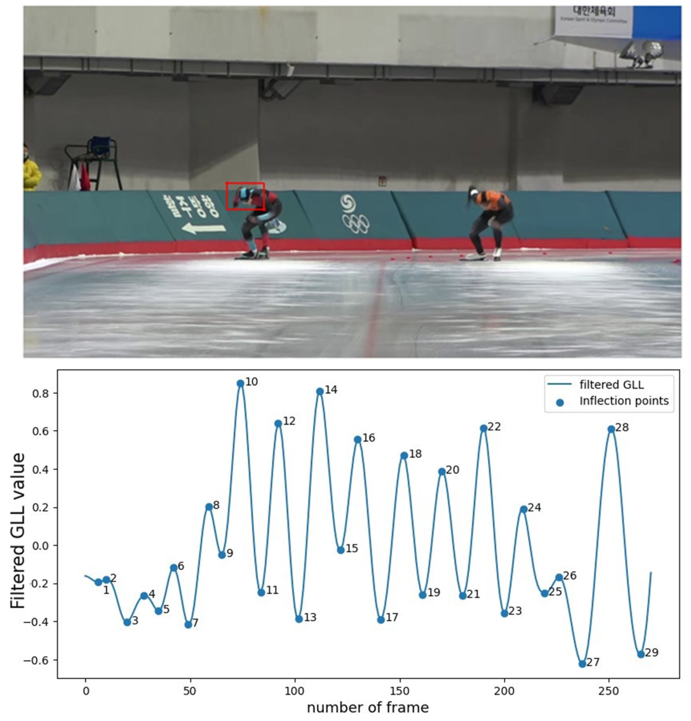
Figure 22.
Player 2: experimental results. A bounding box is drawn around Player 2’s face (top) and inflection point positions extracted from the GLL signal obtained from Player 2 and the stroke count at each of these positions (bottom). As can be seen in the top image, the video of the player on the left side of the screen is used. This figure addresses the case where Player 2’s stroke counts do not match the correct answers.
Table 1 summarizes the experimental results. At this time, the total error sum is the sum of the differences between the number of actual strokes in the 10 experiments and the number measured by the method proposed in this study. The correct rate was calculated using Equation (4).

Table 1.
Experimental results for frontal-view videos. The experiment was conducted on a total of four skaters, and 10 experiments were conducted for each skater to obtain the number of errors compared to total strokes. As a result, the correct rate is calculated and displayed for each player.
For videos captured from the side, the experiment was conducted in the same manner as for videos captured from the front. Two videos were captured from each side and 10 experiments were conducted per video. Table 2 presents the results of the experiment using videos captured from the side.
Table 2.
Experimental results for side-view videos. The experiment was conducted on a total of two players, and 10 experiments were conducted for each player to obtain the number of errors compared to total strokes. As a result, the correct rate is calculated and displayed for each player.
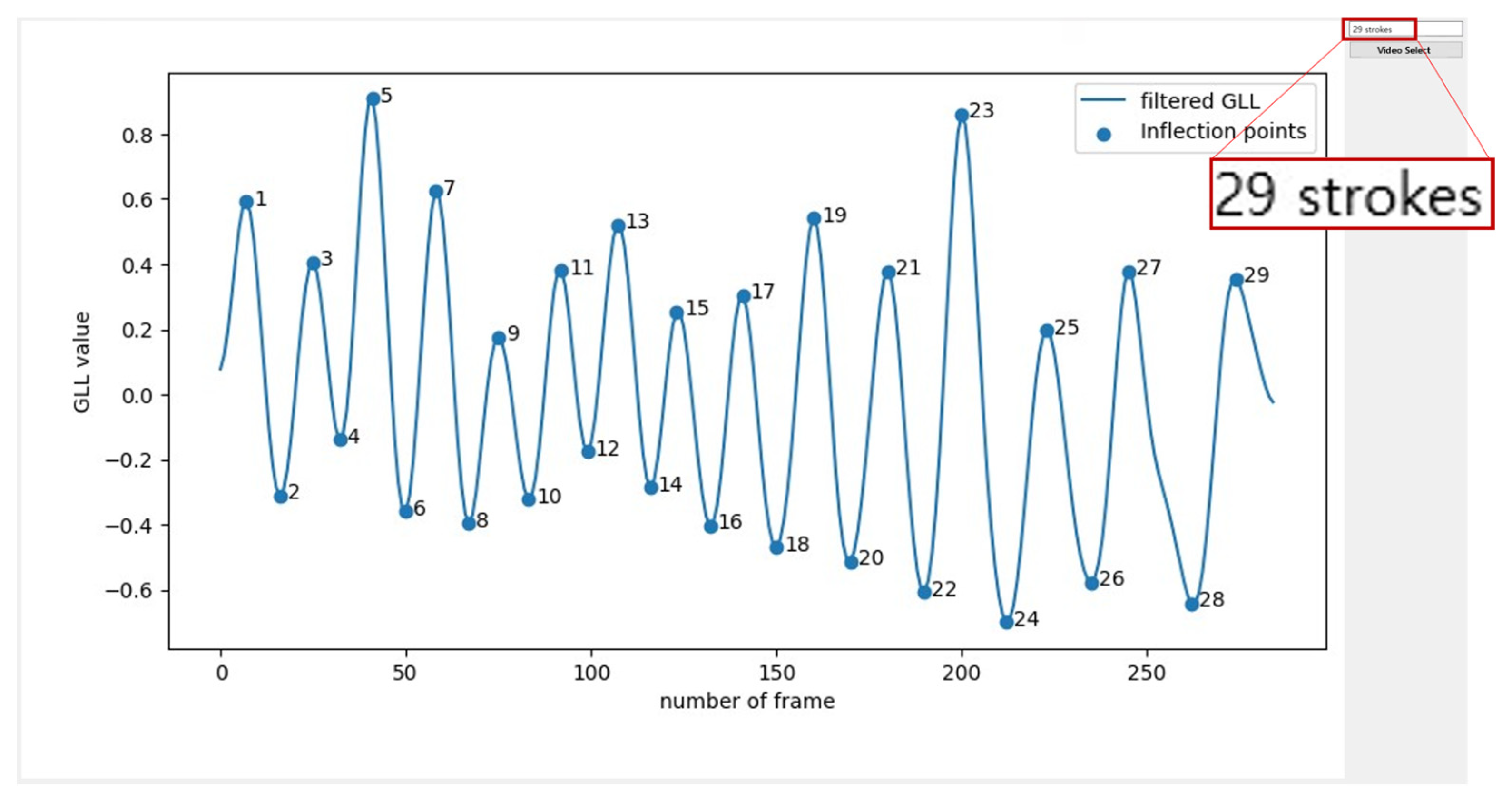
Figure 23, Figure 24 and Figure 25 detail the execution screens of the actual implementation of the proposed method. The UI in Figure 25 was implemented using PyQt, a graphic user interface framework in Python.

Figure 23.
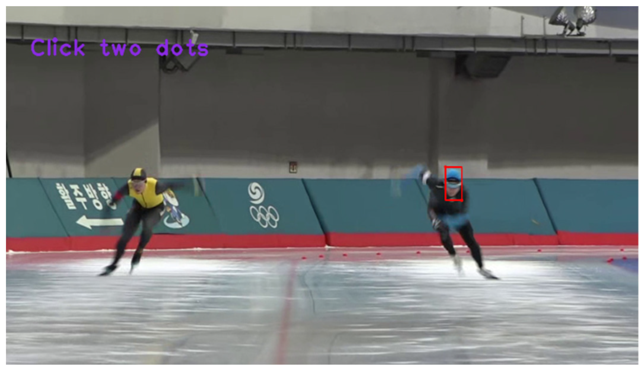
Entering the user’s measurement target ROI. In this figure, the video of the player on the left side of the screen is used. The red frame represents the head area of the measurement target specified by the user in the first frame.
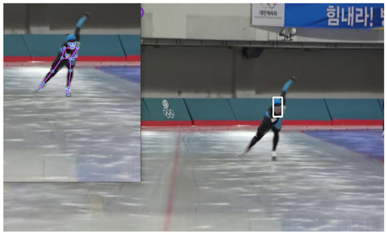
Figure 24.
Player tracking and crop; landmark coordinate tracking. The white frame represents the head region tracked in each frame.
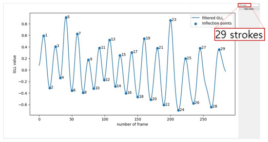
Figure 25.
Measurement results. The blue lines represent the value of the filtered GLL signal, and the dots represent the points corresponding to the number of strokes.
5. Discussion
This study’s results demonstrate a promising achievement with a remarkable correctness rate of 99.91% in frontal-view videos and with only 1 stroke missed out of 1170 strokes. This success underscores the system’s accuracy and consistency, fulfilling the original goal of the research. Minimal user intervention is required, limited to providing the stroke video and bounding box for the measurement target, enhancing the system’s usability even in situations where users may not fully understand its operation.
However, the correctness rate decreased to 96.56% when examining side-view videos. Several factors can be attributed to this decrease: First, side-view videos often contain objects that obscure the measurement target, leading to increased noise in the landmark extraction. The noise-filtering process can only achieve a certain amount in such cases. Second, there is a higher likelihood of capturing unintended persons outside the track, causing the extraction of landmarks from the wrong individuals. This complicates the extraction of purely target-related data.
It is worth noting that the system was primarily designed for front-facing videos. While results from side-view experiments were less robust, the system’s applicability still remains meaningful for front-facing measurements. Therefore, within the constraints of a front-facing measurement environment, the system effectively replaces conventional stroke number measurement methods.
Future research opportunities lie in further exploring the potential of the GLL indicator and its application to speed skating training. The indicator can provide valuable insights into an athlete’s motion quality. Expanding on this work, additional indicators could be developed to enhance training techniques. This study demonstrates that 2D camera-based motion recognition technology is viable for speed skating and offers possibilities for its broader application in various aspects of the sport.
6. Conclusions
In conclusion, this study showcased the successful automation of stroke counting within the initial 100 m segment of speed skating, utilizing MediaPipe Pose landmark data, in particular the GLL indicator. The suggested system exhibited exceptional accuracy with a 99.91% correctness rate in frontal-view videos, highlighting its remarkable precision and reliability. However, when dealing with side-view videos, the accuracy showed a slight decline to 96.56%, primarily due to the inherent challenges associated with such footage.
It is important to emphasize that the suggested system was primarily designed and optimized for front-facing videos. Within this specific context, it provides an effective and user-friendly alternative to traditional stroke-counting methods.
Furthermore, this research has unveiled the potential of the GLL indicator in assessing an athlete’s motion quality, which opens the door to further exploration in speed skating training techniques.
In summary, this study underscores the effectiveness of 2D camera-based motion recognition technology in the field of speed skating. It not only advances understanding of the sport but also hints at broader applications. As technology continues to evolve, we anticipate ongoing refinements to the system, making it even more valuable in the realm of sports analysis.
Author Contributions
Conceptualization, Y.-J.P., J.-Y.M. and E.C.L.; material preparation, data collection, and analysis, Y.-J.P., J.-Y.M. and E.C.L.; writing—original draft, Y.-J.P.; writing—review and revision, E.C.L. All authors have read and agreed to the published version of the manuscript.
Funding
This research was supported by a 2023 research grant from Sangmyung University.
Institutional Review Board Statement
The study was conducted according to the guidelines of the Declaration of Helsinki, and approved by the Institutional Review Board of Sangmyung University (SMUIRB (C-2023-005), 5 July 2023)
Informed Consent Statement
Informed consent was obtained from all subjects involved in the study.
Data Availability Statement
As these are data relating to actual athletes, the data cannot be disclosed except for the purposes of this study.
Conflicts of Interest
The authors declare that they have no conflict of interest.
References
- Purevsuren, T.; Khuyagbaatar, B.; Kim, K.; Kim, Y.H. Investigation of Knee Joint Forces and Moments during Short-Track Speed Skating Using Wearable Motion Analysis System. Int. J. Precis. Eng. Manuf. 2018, 19, 1055–1060. [Google Scholar] [CrossRef]
- de Koning, J.J.; van Ingen Schenau, G.J. Performance-Determining Factors in Speed Skating. In Biomechanics in Sport; Blackwell Science Ltd.: Oxford, UK, 2008; pp. 232–246. ISBN 9780470693797. [Google Scholar]
- Kim, G.-T.; Ryu, J.-K. An Analysis of the Determinants of Performance for the Curves in Official Speed Skating 500m Race. Korean J. Phys. Educ. 2021, 60, 189–203. [Google Scholar] [CrossRef]
- de Boer, R.W.; Nilsen, K.L. Work per Stroke and Stroke Frequency Regulation in Olympic Speed Skating. Int. J. Sport Biomech. 1989, 5, 135–150. [Google Scholar] [CrossRef]
- Kimura, Y.; Yokozawa, T.; Maeda, A.; Yuda, J. Changes in Straight Skating Motions in World-Class Long-Distance Speed Skaters during the Ladies’ 3,000-m Race. Int. J. Sport Health Sci. 2022, 20, 37–47. [Google Scholar] [CrossRef]
- Yeonjonglee, N. Analysis of the 2000. World Sprint Speed Skating Championship. Korean J. Phys. Educ. 2001, 40, 975–982. [Google Scholar]
- Burkhardt, D.; Born, D.-P.; Singh, N.B.; Oberhofer, K.; Carradori, S.; Sinistaj, S.; Lorenzetti, S. Key Performance Indicators and Leg Positioning for the Kick-Start in Competitive Swimmers. Sports Biomech. 2023, 22, 752–766. [Google Scholar] [CrossRef]
- Herold, M.; Kempe, M.; Bauer, P.; Meyer, T. Attacking Key Performance Indicators in Soccer: Current Practice and Perceptions from the Elite to Youth Academy Level. J. Sports Sci. Med. 2021, 20, 158–169. [Google Scholar] [CrossRef]
- Hughes, M.; Caudrelier, T.; James, N.; Donnelly, I.; Kirkbride, A.; Duschesne, C. Moneyball and Soccer—An Analysis of the Key Performance Indicators of Elite Male Soccer Players by Position. J. Hum. Sport Exerc. 2012, 7, 402–412. [Google Scholar] [CrossRef]
- Boyd, C.; Barnes, C.; Eaves, S.J.; Morse, C.I.; Roach, N.; Williams, A.G. A Time-Motion Analysis of Paralympic Football for Athletes with Cerebral Palsy. Int. J. Sports Sci. Coach. 2016, 11, 552–558. [Google Scholar] [CrossRef]
- Bourdon, P.C.; Cardinale, M.; Murray, A.; Gastin, P.; Kellmann, M.; Varley, M.C.; Gabbett, T.J.; Coutts, A.J.; Burgess, D.J.; Gregson, W. Monitoring Athlete Training Loads: Consensus Statement. Int. J. Sports Physiol. Perform. 2017, 12, S2-161–S2-170. [Google Scholar] [CrossRef]
- Seshadri, D.R.; Drummond, C.; Craker, J.; Rowbottom, J.R.; Voos, J.E. Wearable Devices for Sports: New Integrated Technologies Allow Coaches, Physicians, and Trainers to Better Understand the Physical Demands of Athletes in Real Time. IEEE Pulse 2017, 8, 38–43. [Google Scholar] [CrossRef]
- Li, B.; Xu, X. Application of Artificial Intelligence in Basketball Sport. J. Educ. Health Sport 2021, 11, 54–67. [Google Scholar] [CrossRef]
- Zhao, L.; Pan, D. Video Analysis of Belt and Road Sports Events Based on Wireless Network and Artificial Intelligence Technology. Wirel. Commun. Mob. Comput. 2022, 2022, 8278045. [Google Scholar] [CrossRef]
- Chu, W.C.-C.; Shih, C.; Chou, W.-Y.; Ahamed, S.I.; Hsiung, P.-A. Artificial Intelligence of Things in Sports Science: Weight Training as an Example. Computer 2019, 52, 52–61. [Google Scholar] [CrossRef]
- Wright, Z.A.; Patton, J.L.; Huang, F.C.; Lazzaro, E. Evaluation of Force Field Training Customized According to Individual Movement Deficit Patterns. In Proceedings of the 2015 IEEE International Conference on Rehabilitation Robotics (ICORR), Singapore, 11–14 August 2015; pp. 193–198. [Google Scholar]
- Huber, S.K.; Held, J.P.O.; de Bruin, E.D.; Knols, R.H. Personalized Motor-Cognitive Exergame Training in Chronic Stroke Patients—A Feasibility Study. Front. Aging Neurosci. 2021, 13, 730801. [Google Scholar] [CrossRef] [PubMed]
- Dellaserra, C.L.; Gao, Y.; Ransdell, L. Use of Integrated Technology in Team Sports: A Review of Opportunities, Challenges, and Future Directions for Athletes. J. Strength Cond. Res. 2014, 28, 556–573. [Google Scholar] [CrossRef]
- Castellano, J.; Casamichana, D. Heart Rate and Motion Analysis by GPS in Beach Soccer. J. Sports Sci. Med. 2010, 9, 98–103. [Google Scholar]
- Wundersitz, D.; Gastin, P.; Robertson, S.; Davey, P.; Netto, K. Validation of a Trunk-Mounted Accelerometer to Measure Peak Impacts during Team Sport Movements. Int. J. Sports Med. 2015, 36, 742–746. [Google Scholar] [CrossRef] [PubMed]
- Cao, Z.; Hidalgo, G.; Simon, T.; Wei, S.-E.; Sheikh, Y. OpenPose: Realtime Multi-Person 2D Pose Estimation Using Part Affinity Fields. arXiv 2018, arXiv:1812.08008. [Google Scholar] [CrossRef]
- Xu, Y.; Zhang, J.; Zhang, Q.; Tao, D. ViTPose: Simple Vision Transformer Baselines for Human Pose Estimation. arXiv 2022, arXiv:2204.12484. [Google Scholar] [CrossRef]
- Shi, D.; Wei, X.; Li, L.; Ren, Y.; Tan, W. End-to-End Multi-Person Pose Estimation with Transformers. In Proceedings of the 2022 IEEE/CVF Conference on Computer Vision and Pattern Recognition (CVPR), New Orleans, LA, USA, 18–24 June 2022; pp. 11069–11078. [Google Scholar]
- Li, K.; Wang, S.; Zhang, X.; Xu, Y.; Xu, W.; Tu, Z. Pose Recognition with Cascade Transformers. arXiv 2021, arXiv:2104.06976. [Google Scholar] [CrossRef]
- Panteleris, P.; Argyros, A. PE-Former: Pose Estimation Transformer. In Pattern Recognition and Artificial Intelligence; Springer International Publishing: Cham, Switzerland, 2022; pp. 3–14. ISBN 9783031092817. [Google Scholar]
- Ma, J.; Ma, L.; Ruan, W.; Chen, H.; Feng, J. A Wushu Posture Recognition System Based on MediaPipe. In Proceedings of the 2022 2nd International Conference on Information Technology and Contemporary Sports (TCS), Guangzhou, China, 24–26 June 2022; pp. 10–13. [Google Scholar]
- Zhang, Y. Applications of Google MediaPipe Pose Estimation Using a Single Camera. Master’s Thesis, California State Polytechnic University, Pomona, CA, USA, 2022. [Google Scholar]
- Gao, L.; Zhang, G.; Yu, B.; Qiao, Z.; Wang, J. Wearable Human Motion Posture Capture and Medical Health Monitoring Based on Wireless Sensor Networks. Measurement 2020, 166, 108252. [Google Scholar] [CrossRef]
- Kim, W.; Kim, M. On-Line Detection and Segmentation of Sports Motions Using a Wearable Sensor. Sensors 2018, 18, 913. [Google Scholar] [CrossRef] [PubMed]
- Pajak, G.; Krutz, P.; Patalas-Maliszewska, J.; Rehm, M.; Pajak, I.; Dix, M. An Approach to Sport Activities Recognition Based on an Inertial Sensor and Deep Learning. Sens. Actuators A Phys. 2022, 345, 113773. [Google Scholar] [CrossRef]
- Rahmadani, A.; Bayu Dewantara, B.S.; Sari, D.M. Human Pose Estimation for Fitness Exercise Movement Correction. In Proceedings of the 2022 International Electronics Symposium (IES), Surabaya, Indonesia, 9–11 August 2022; pp. 484–490. [Google Scholar]
- Kulkarni, K.M.; Shenoy, S. Table Tennis Stroke Recognition Using Two-Dimensional Human Pose Estimation. arXiv 2021, arXiv:2104.09907. [Google Scholar] [CrossRef]
- Einfalt, M.; Zecha, D.; Lienhart, R. Activity-Conditioned Continuous Human Pose Estimation for Performance Analysis of Athletes Using the Example of Swimming. In Proceedings of the 2018 IEEE Winter Conference on Applications of Computer Vision (WACV), Lake Tahoe, NV, USA, 12–15 March 2018; pp. 446–455. [Google Scholar]
- Bazarevsky, V.; Grishchenko, I.; Raveendran, K.; Zhu, T.; Zhang, F.; Grundmann, M. BlazePose: On-Device Real-Time Body Pose Tracking. arXiv 2020, arXiv:2006.10204. [Google Scholar] [CrossRef]
- Brdjanin, A.; Dardagan, N.; Dzigal, D.; Akagic, A. Single Object Trackers in OpenCV: A Benchmark. In Proceedings of the 2020 International Conference on INnovations in Intelligent SysTems and Applications (INISTA), Novi Sad, Serbia, 24–26 August 2020; pp. 1–6. [Google Scholar]
- Lukežič, A.; Vojíř, T.; Čehovin Zajc, L.; Matas, J.; Kristan, M. Discriminative Correlation Filter Tracker with Channel and Spatial Reliability. Int. J. Comput. Vis. 2018, 126, 671–688. [Google Scholar] [CrossRef]
- Brigham, E.O.; Morrow, R.E. The Fast Fourier Transform. IEEE Spectrum. 1967, 4, 63–70. [Google Scholar] [CrossRef]


Disclaimer/Publisher’s Note: The statements, opinions and data contained in all publications are solely those of the individual author(s) and contributor(s) and not of MDPI and/or the editor(s). MDPI and/or the editor(s) disclaim responsibility for any injury to people or property resulting from any ideas, methods, instructions or products referred to in the content. |
© 2023 by the authors. Licensee MDPI, Basel, Switzerland. This article is an open access article distributed under the terms and conditions of the Creative Commons Attribution (CC BY) license (https://creativecommons.org/licenses/by/4.0/).