Abstract
The port container gantry crane studied in this paper is a four-degree-of-freedom spatial continuous system. In actual work, in order to make the container transfer smoothly, the response of the whole system needs to be accurately predicted and timely adjusted. The whole system is divided into rotary mechanism, lifting mechanism, lifting trolley mechanism, and big cart mechanism for detailed analysis. By constructing the field transfer matrix, a one-dimensional wave equation of continuous system and the Lagrange equation with redundant parameters, the response of each subsystem is solved precisely. The results of the study found that in some periods, the swing of the container was too large. In order to improve the safety and stability of transmission, an active control method of specific point in time excitation (SPE) is proposed for the first time. This method predicts the swing amplitude of the container in advance using the response results of the numerical model. When the set response interval is exceeded, the external excitation intervention can effectively inhibit the moving range of the container in the transit process. Finally, the results are compared with the simulation model to achieve the experimental purpose. It is in line with the expected experimental effect.
1. Introduction
Since the 21st century, the Internet of Things technology has developed rapidly, and logistics intelligence has become more and more important in port construction. With the advent of the 5G era, port intelligent traffic and remote control technology have reached a greater level. Pham Thi Yen’s research provides insights into key trends and future research directions for smart ports [1]. Yan Zhang pointed out that due to the continuous progress and application of information technology, the digital transformation of intelligent logistics and supply chain management has become an inevitable trend [2].
Many experts and scholars have conducted in-depth discussion and research on the construction of future smart ports. Johannes Benkert explores whether lidar systems in automated container terminals (ACTS) can be replaced by cameras, the foundations of automated container terminals, existing automation solutions and sensor technologies, and the opportunities and challenges of the transition from lidar to cameras. Donta Praveen Kumar proposes a big data approach that can aid in the sustainable operation of port container crane systems [3,4]. Casamayor Pujol Victor discusses representations, models, lifelong learning, and business models for distributed computing continuous systems, and proposes a new approach that can be applied to container gantry cranes [5]. The logistics system is an important part of unmanned ports, and the swing control of containers can be considered as the key here. An enhanced coupled time-varying sliding mode control method is designed to eliminate the arrival phase of the sliding mode control method, and a perturbation bound is constructed for the global robustness of max-plus linear systems to ensure that parameter perturbations within the perturbation boundary do not affect the original state and output. By considering an anti-roll control of the fuzzy sliding surface of a container crane, a coupling sliding surface is proposed to ensure the asymptotic stability of the closed-loop system. They used an adaptive gain sliding mode control (SMC) scheme to propose load placement and container positioning problems for ship container cranes [6,7,8,9]. The fuzzy PID anti-roll controller and an input shaper with adaptive scheme proposed by some experts and scholars can not only improve the adaptability of the control system, but also overcome the large overthrow and quickly suppress the swing, effectively realizing the anti-roll function of the bridge crane [10,11]. The experts also studied anti-swing controls of two-link planes. A proportional derivative (PD) controller using a damper and a linear spring with positive stiffness and a sine derivative (SD) controller using a damper and a nonlinear spring with negative stiffness are proposed. Finally, it is proved that when the linear or nonlinear stiffness of a spring meets certain conditions, the control target can be achieved [12]. Some scholars have proposed two switching control methods to realize the control of self-assembled inverted pendulum, aiming at solving two important problems of self-assembled inverted pendulum: oscillating and stabilizing in its upright equilibrium position. At the same time, it is considered that the swing of lifting loads and the positioning of the trolley during the operation of a crane seriously affect its safety and reliability. A proportional integral differential controller is designed for anti-swing and positioning control, and a hybrid particle swarm optimization and simulated annealing algorithm are proposed to optimize the gain of the controller. A coordinated control method between the track and trolley of double-pendulum cranes is also proposed, which improves the working efficiency of double-pendulum cranes and realizes the anti-pendulum control of them in a three-dimensional motion mode [13,14,15].
In order to improve the intelligent level of port logistics systems, many experts and scholars have also proposed specific control methods to improve the swing of containers during transportation. They proposed a type 2 fuzzy PID controller for bridge crane systems to improve position control and suppress load oscillations. At the same time, dynamic analysis of DMB double-swing cranes is carried out, and the time-optimal anti-swing control method is improved, and the minimum and maximum residual angles are achieved using low-pass filters to smooth the velocity trajectory to avoid collision [16,17]. Some experts have proposed a method of modeling and nonlinear sliding mode control for double-pendulum cranes which takes into account mass beam distribution, rope length variation, and external disturbance. This control method can ensure the asymptotic stability of a system in finite time, maintain robustness under disturbance, and adapt to changes in rope length. They have created a new model-free robust control scheme for payload swing angle attenuation in a variable rope length 2D crane system. Rigorous stability analysis shows that the proposed controller enables the system to follow the desired translational motion and oscillation to lift and reduce loads with smaller loads. In order to effectively suppress the swing of a load, a swing control method based on the predictive unit amplitude shaper and adaptive feedback control is proposed [18,19,20]. By combining the inverse pendulum feedback damping of an all-state crane with the reference trajectory, a real-time correction trajectory planning method of tower cranes with dropping/lifting load movement is proposed. They also proposed, for the first time, the modeling of a double-ship crane and the design of an output feedback controller. The designed controller can realize the precise positioning of double-constrained derricks and effectively eliminate load swing. Some scholars introduced an anti-swing controller of hydraulic loader cranes, and verified the performance of the anti-swing controller with experiments. Some experts have studied the H∞ output feedback anti-swing controller for a class of nonlinear bridge crane systems with external interference. In practical applications, it has shown good load angle inhibition effect [21,22,23,24].
In addition to the research on the swing of lifting objects, many researchers also further study the whole lifting system from the impact on the surrounding environment, which is of great significance for the construction of unmanned ports. They studied the effectiveness of six seismic reinforcement interventions for existing large container cranes. The influence of seismic frequency on the seismic response of typical modern container cranes is also studied. Shaking table tests are carried out on a crane constructed according to the law of similarity to study the seismic response of a container crane. Based on the aerodynamic data obtained from wind tunnel tests, the dynamic transient wind-induced sliding force and tilting moment response of container cranes on shore were analyzed. Aiming at the problems of a lack of an online data simulation test environment, poor openness of data collection, and a low degree of data visualization in the online control process of port cranes, some scholars proposed a port crane operation status monitoring system framework based on digital twins [25,26,27,28,29].
The response control caused by the overall working state of cranes is also the research focus of many experts and scholars. Aiming at the coupled vibration of the wheel–rail–beam system of high-speed shore container cranes, they have found out the measures required to reduce the vibration of high-speed operation of container cranes. A comprehensive framework for structural model verification and reliability evaluation is also constructed [30,31]. Scholars have created a continuous integral sliding mode control method for ship container cranes under input saturation conditions to suppress swing [32]. An adaptive input shaper is proposed to solve the oscillating problem of 5-DOF tower cranes under various parameters of uncertainty, load lifting, and synchronous motion. Input shaping and radial spring damping are also combined to reduce three-way vibration of crane loads [33,34]. Experts widely use underactuated mechanical systems as experimental devices to interpret and test various control algorithms, which have certain reference significance for the swing generated during crane operation [35]. The authors integrate the irregular wave model into the dynamic model of a three-time roll stabilization system, and simplify the three-time roll stabilization system with lifting load at sea into a constrained pendulum system with dynamic base excitation. A three-dimensional online trajectory planning method for offshore cranes is also proposed to attenuate or eliminate unwanted cargo swings due to improper crane operation and ship motion interference [36,37]. Considering transportation time, energy consumption, and all state constraints, an optimal trajectory planning strategy for bridge cranes is proposed, which takes pendulum mechanics into account. They also model and analyze the transformation of the cable-driven inverse tetrahedral mechanism of Marine cranes. Aiming at stability control of double pendulum Marine cranes under the conditions of matching disturbance, unmatching disturbance, and actuator saturation, an anti-pendulum partial saturation control method is created. The closed-loop asymptotic stability is strictly proved. Aiming at the problem that large swing amplitude may occur when lifting loads, resulting in inaccurate positioning and low transportation efficiency, a new nonlinear coupled tracking anti-swing controller of double-pendulum gantry cranes is proposed, which effectively inhibits and eliminates the swing angle of hooks and loads [38,39,40,41].
The author consulted a lot of data and found that there are still some improvements in the theoretical research of port container gantry cranes in the development of smart port logistics. The existing research content can continue to explore and improve the response analysis of a four-degree-of-freedom crane system. Therefore, different from the synovial control methods proposed by many experts and scholars, this paper constructs a new method which can actively control the swing of containers using mechanism analysis of cranes. The time and amplitude of the swing are predicted in advance with numerical calculation of the agent model. Finally, the excitation of the system is adjusted to further control the oscillation of containers in a reasonable range.
In this paper, the authors set up dynamic equations of four kinds of mechanisms with time as a one-dimensional function and calculate the response of each kind of mechanism in the specified time period. Finally, the SPE method is proposed, and it is proved that this method has a good control effect on the response of containers in the process of transfer. Firstly, the lifting system of a container crane is analyzed, and it is pointed out that the lifting system mainly causes longitudinal vibration of the container along the lifting direction. For the analysis of the rotating device, the author solves the rotating response by constructing the space field transfer matrix. Based on analysis of a crane trolley, the author divides its motion into two parts: vibration along the beam section of the track and the swing of the container. Finally, the motion of the crane is analyzed, considering that the crane part is not directly connected with the container, so only the swing of the container caused by the working of this part of the system is solved.
2. Response of the Container Gantry Crane in the System Setting State
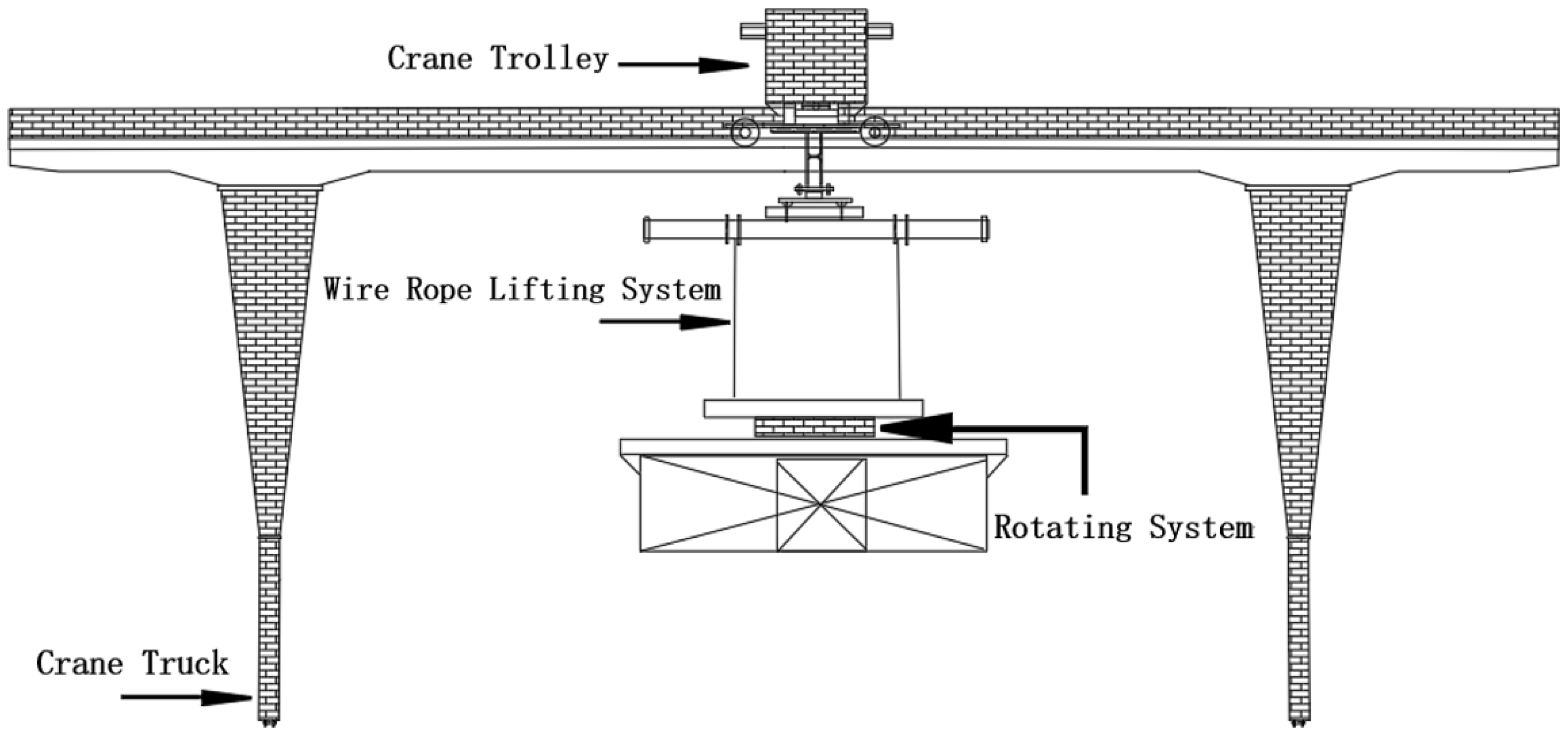
In order to better describe the technical route, Figure 1 is a simplified two-dimensional plane diagram of a container gantry crane. It can be seen from the two-dimensional container simplified diagram that the author divides the experimental container gantry crane into four parts according to the motion sequence: wire rope lifting system, rotating system, lifting trolley operating mechanism, and large truck operating mechanism. To facilitate the next model, check calculation. Table 1 shows the basic parameters of container gantry cranes.
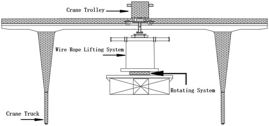
Figure 1.
Simplified schematic diagram of container gantry crane.

Table 1.
Technical parameters of container gantry crane.
The M6 (M7) work level in the table above is related to the parameters of this experimental model. It represents a heavy material handling mechanism with high operating frequency and high strength. The determination of the working level is related to the operating environment of each subsystem, such as running speed, lifting weight, and load coefficient.
2.1. The Solution of the Response of Rotary Mechanism in the Initial Setting State
As can be seen from Figure 1, the lower end of the rotating bearing is connected to the container, and the upper end is connected to the drum fixed on the lifting trolley with wire rope. On the basis of constructing a dynamic equation, it is necessary to express the rigid–flexible coupling phenomenon between wire rope and the rigid body connected at the upper and lower ends. According to the mechanical relation, the field transfer matrix is constructed, and the response of this part of the continuous system in the initial state is obtained.
The excitation of the rotating mechanism to the container in the initial state is regarded as a single cycle. Fourier transform is performed after the expression of excitation equivalence. The rated speed of the known rotating device is 2 r*min−1, and the treated dynamic equation is expressed as follows.
In the above equation, represents the moment of inertia of the container parallel to the car. , represents the corresponding damping and stiffness, respectively. represents the number of sampling points in the response converted to the Fourier transform.
Next, the transfer matrix of the rotating mechanism is established. First, define the state variable.
In the above formula, represents the angle in the initial state. represents the torque in the initial state.
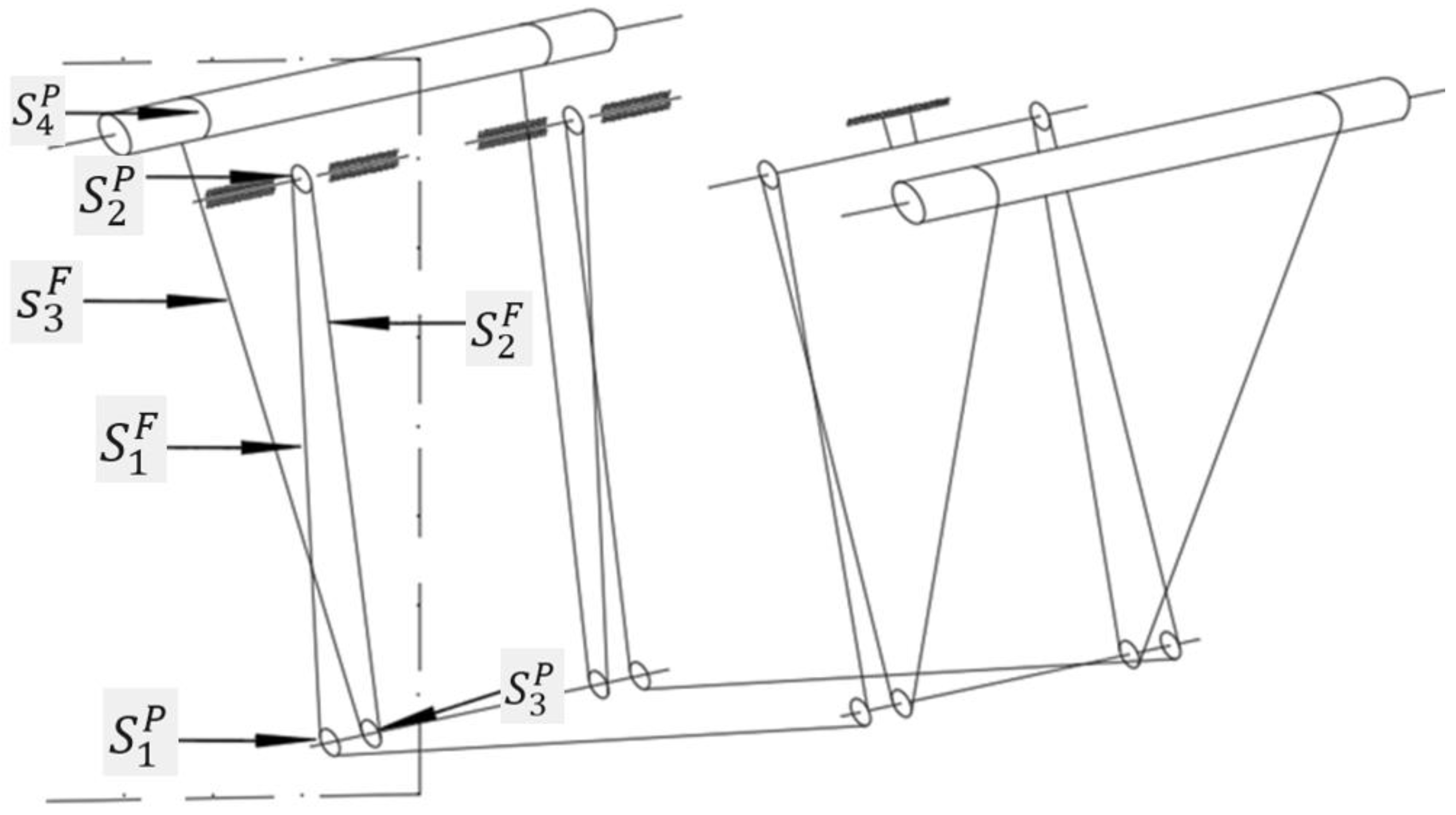
Mechanical assumptions are made about the wire rope reel in Figure 2. Firstly, the input direction of the single-degree-of-freedom rotating system is analyzed. Set at the wire rope contact reel torque changes, the angle remains unchanged. Set at the point transfer matrix here, the following relationship is satisfied.

Figure 2.
Schematic diagram of wire rope winding.
Figure 2.
Schematic diagram of wire rope winding.
is the expression of the point transfer matrix.
The angle of two coils connecting the same section of wire rope changes correspondingly, the torque remains unchanged, and the field transfer matrix is set between the sections of wire rope. Similar to the above method, the field transfer matrix satisfies the following relationship:
is the expression of the field transfer matrix.
According to the winding order of the wire rope, the following relationship exists between the output ends of the wire rope of the adjacent two coils:
The author substituted the rotation speed set by the rotary system as the initial condition. The boundary conditions of container joints are obtained. The analytical solution at the exit of each wire rope drum is calculated. See Appendix A for relevant analysis. The boundary conditions of the connection between the wire rope and the drum in the initial state are brought into the formula in Appendix A, which is convenient for further solving the natural frequency and mode function. and in Appendix A are the boundary conditions of the wire rope system in its initial state.
According to the above formula, the exponential term containing the initial state is not considered for the time being. By observing the winding mode of the wire rope in Figure 2, it can be seen that the rotation angle of the wire rope at node 2 and node 4 is zero under the indicated state. Bring the boundary conditions into the transfer matrix and Appendix A to find the natural angular frequency of the rotating system. Finally, the fourth natural frequency is obtained.
The modal superposition method is used to solve the rotating response of the container at a specified height. represents the rotational stiffness of the wire rope. represents the moment of inertia of the wire rope at a given height at a given time.
When solving the response of a single-degree-of-freedom rotating device, it can be divided into the free vibration stage of forced excitation, transition stage, and steady state response stage. After acquiring the data, the relative damping coefficient is preliminarily set as 0.1.
We know that in the initial state, the angular coordinate is zero, and the initial angular velocity is . The analysis of single-degree-of-freedom damped free vibration, of transition state, and of steady state are obtained, successively.
In the above formula, represents the amplitude of the system excitation force in the initial state. represents the ratio of the external excitation frequency to the natural frequency of the system. indicates the distance from the point of operation of the wire rope to the centroid on the container.
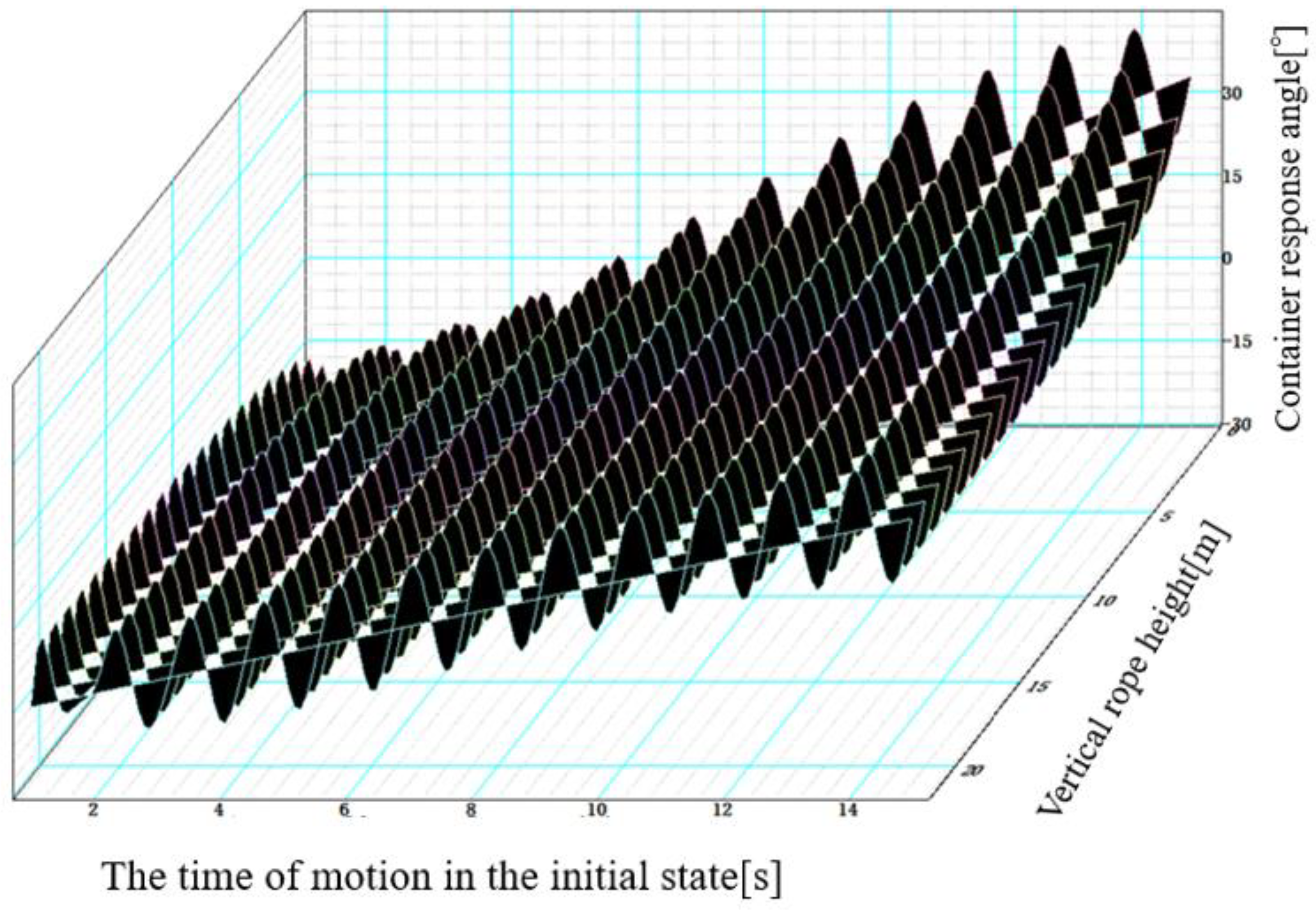
Above is the response of the crane rope rotation system. According to the design condition, the container rotates 90 degrees for one cycle, bringing in the correlation coefficient. Figure 3 shows the response of the container under system excitation.
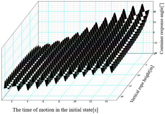
Figure 3.
Container response under the action of a rotating system.
The Figure 3 shows that under the action of the initial excitation, the angle of the centroid position of the lower end of the container relative to the fixed position of the upper end connected by the wire rope will increase with the extension of action time.
2.2. Response of the Lifting Mechanism in the Initial Setting State of the System
With research of the wire rope lifting mechanism, the rigid–flexible coupling of the lifting system is analyzed. A fixed length of steel wire rope section is selected for mechanical analysis. Figure 4 is a magnified image of a piece of wire rope captured. The longitudinal motion of a container under the excitation of a lifting system is further determined using the structural mechanics equation.
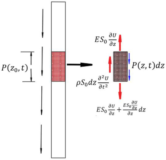
Figure 4.
Magnification of the local force of the wire rope.
The authors need to establish the one-dimensional wave equation of the lifting mechanism. From the mechanical relation of the wound steel wire rope, it can be seen that there is some equivalent relation between the internal force of the steel wire rope in a certain section and the inertia force of D ‘Alembert and the external force applied. The motion law at any point of the wire rope is derived.
In the above formula, represents the section area of the wire rope. indicates the density of the material. stands for elastic modulus. represents the external force applied. The following modal coordinate function relation is satisfied using the separation variable method with analysis.
The equation above represents the longitudinal vibration amplitude of the section where the wire rope meets the container. represents the time function of the lifting mechanism motion. Find the general solution of these two functions.
In order to obtain the natural frequency and mode function of the wire rope lifting system. It is assumed that there is a fixed end at the upper roller, which means that the cross section displacement of the wire rope is zero. The connection between the lower container and the wire rope pulley is the free end. The axial force of the wire rope is balanced with the elastic force.
where is the longitudinal length of the wire rope. Consider the need for repeated lifting and lowering of containers, so this is a function of time. The frequency equation is obtained by solving the equation of boundary conditions. Finally, the mode function of the lifting system can be obtained. The mode principal mass and mode principal stiffness of the wire rope lifting system are obtained.
According to the orthogonality of the principal mode of the continuous system, the function obtained using the method of separating variables is put into the dynamic equation of the lifting system. In the case of known modal coordinates, take the dynamics equation multiplied by the I-order mode function and integrate the length of the wire rope to obtain the following equation.
The longitudinal forced vibration of the wire rope when the container is located at a certain position is solved. The second term on the right side of the above equation is denoted , which represents the generalized force in the physical sense of lifting the coordinates of the system. In order to find the coefficients of the mode function in the lifting system . The orthogonality of principal modes of a continuous system is normalized. The modal generalized force of the lifting system is obtained by further solving:
The solved modal generalized force is brought into the solution result of the modal space equation and finally returned to physical space. The vertical response of the lifting system under the set conditions is obtained.
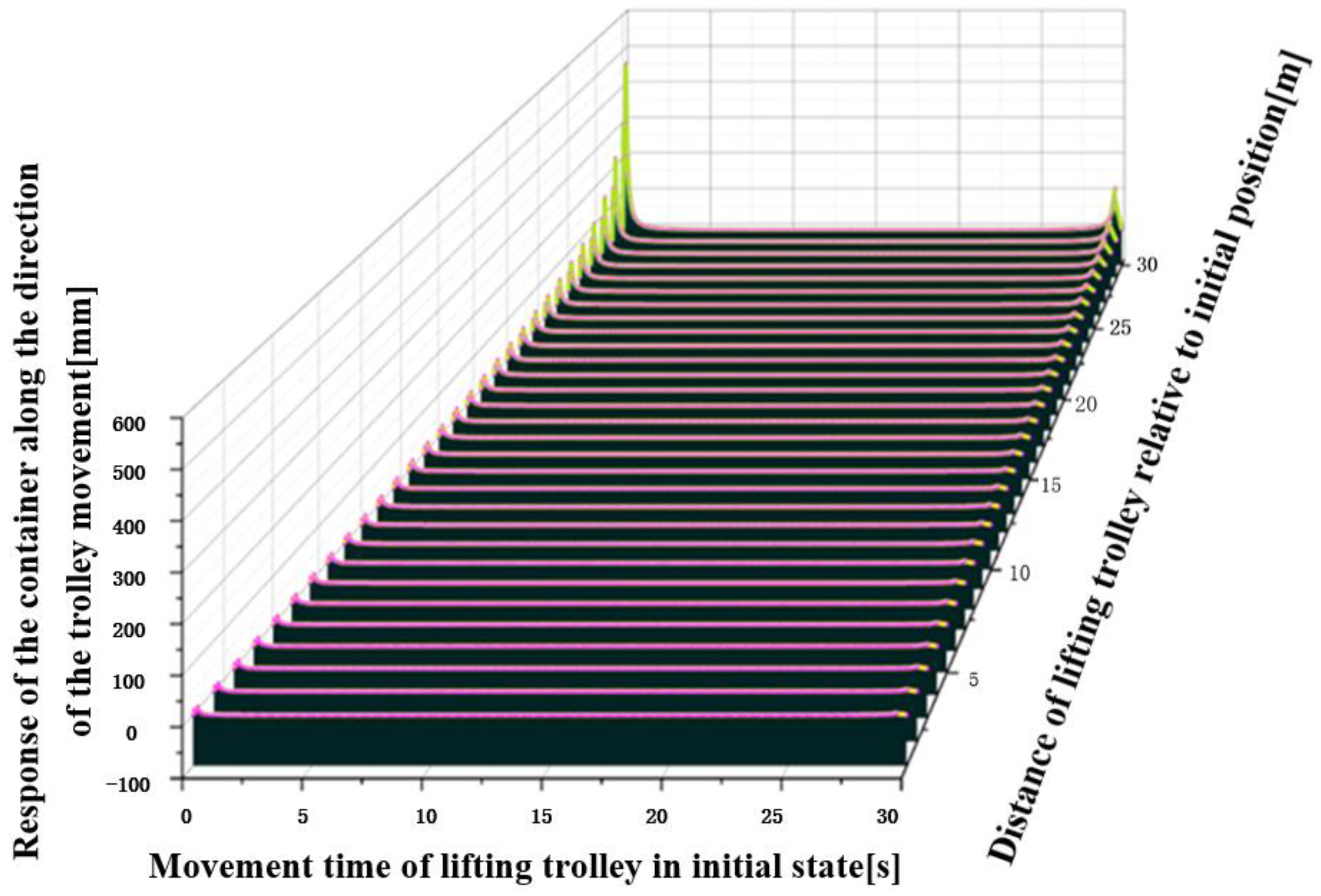
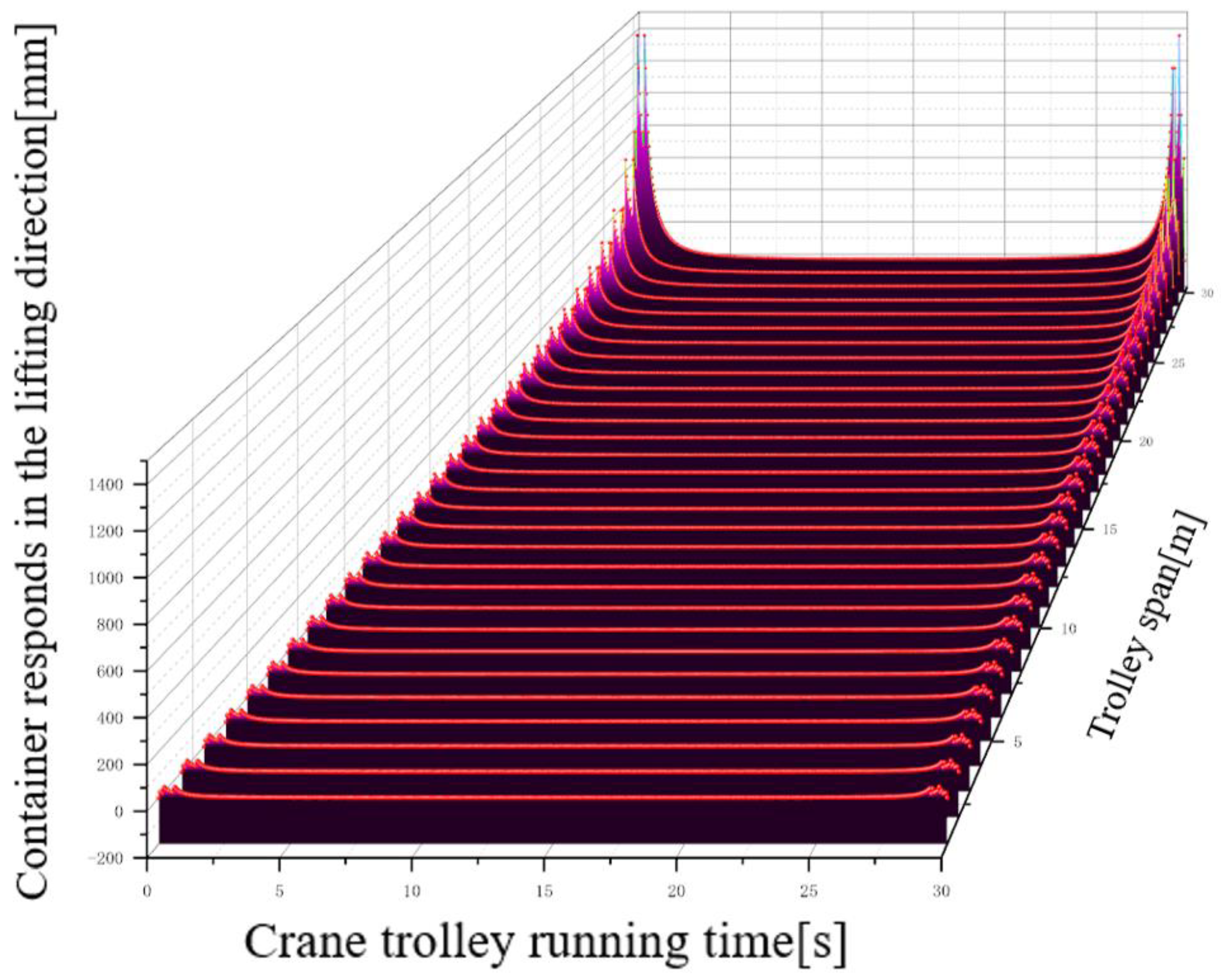
The lifting distance is known. Bring in the lifting speed given in the initial state. The resulting dynamic response image is shown in Figure 5. It can be seen from the figure that in the initial state, no matter which position the lifting trolley is in the track, the container will have large longitudinal vibration, which gradually decreases over time. Eventually it goes to zero. The specific position referred to here is related to the running distance of the lifting trolley on the track. Assuming that the lifting trolley is located at the boundary of the track in the initial state, the maximum distance running is the span size of the track.
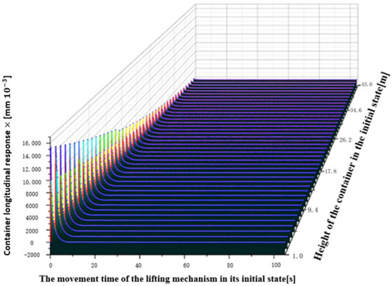
Figure 5.
Container response under lifting system action.
2.3. Crane Trolley Operation Mechanism
The trolley wheels run on rails with fixed beam sections. This part of the response is divided into two parts to solve. The first part is the rolling of the trolley wheel on the track, using the trolley and the connected container as the concentrated mass on the fixed beam section. And assuming that the trolley sliding on the track will cause longitudinal vibration of the beam, the resulting response will be transferred to the container equivalent. The second part is that the movement of the car causes the swing of the container.
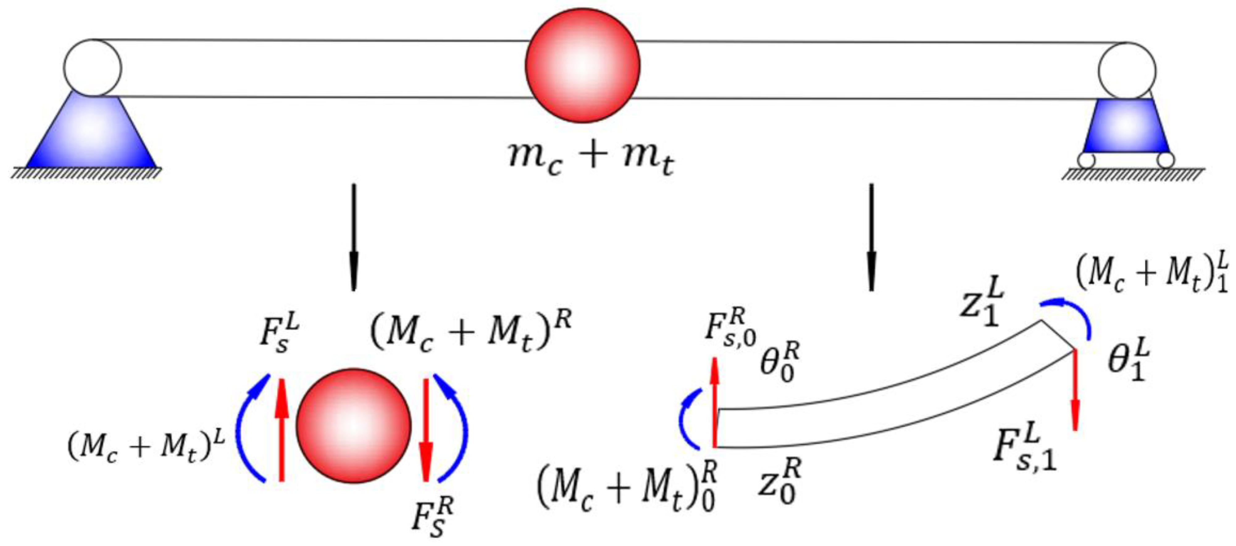
Firstly, the influence of the movement of the lifting trolley on the beam section is considered. The first part of the trolley running mechanism is simplified and analyzed. The other three subsystems of the container crane are in a static state temporarily when decoupling analysis of the running state of the crane trolley is carried out. At this time, the track of the lifting trolley can be regarded as a beam with both ends in a fixed state. Figure 6 shows a simplified mechanical relationship on the section of the rear beam. Ignore the movement of the crane truck for a moment.

Figure 6.
Simplified image when the crane trolley moves in the beam section.
stands for the mass of the container, and stands for the mass of the trolley and the lifting mechanism. Mt and Mc represent the torques for the position of the trolley and container on the track. Fs is the tangential force at the position. The superscripts L and R denote the left and right ends.
On both sides of the concentrated mass, the deflection, angle, and bending moment remain unchanged, and the shear force changes. The point transfer matrix of the trolley mechanism on the beam of a fixed section is constructed. The beam section between the concentrated mass and the boundary constructs the field transfer matrix. The left end of the beam is represented by the left end of the concentrated mass to represent the right end of the specified beam segment. The left end of the specified beam segment is represented by the right end of the concentrated mass. The simplified trolley running mechanism consists of two field transfer matrices and one point transfer matrix. The following is the processed transfer matrix. The numerical expressions for the 16 elements of the matrix are shown in the Appendix B.
The length of the track is the running range of the car. The length is . In the transfer matrix above, and are the left and right ends of the car relative to the track. The sum of these two lengths is equal to the length of the track. They are all a function of time. Bring in the boundary conditions. The angle and bending moment at both ends of the trolley sliding track are zero. The natural frequency of the car at any time is obtained.
According to the running state, the external excitation combined with the Dirac distribution function is expressed.
Remember the start and end time of a single run as a period of aperiodic excitation. The longitudinal bending vibration response of the crane trolley to the beam in the process of moving along the track is obtained.
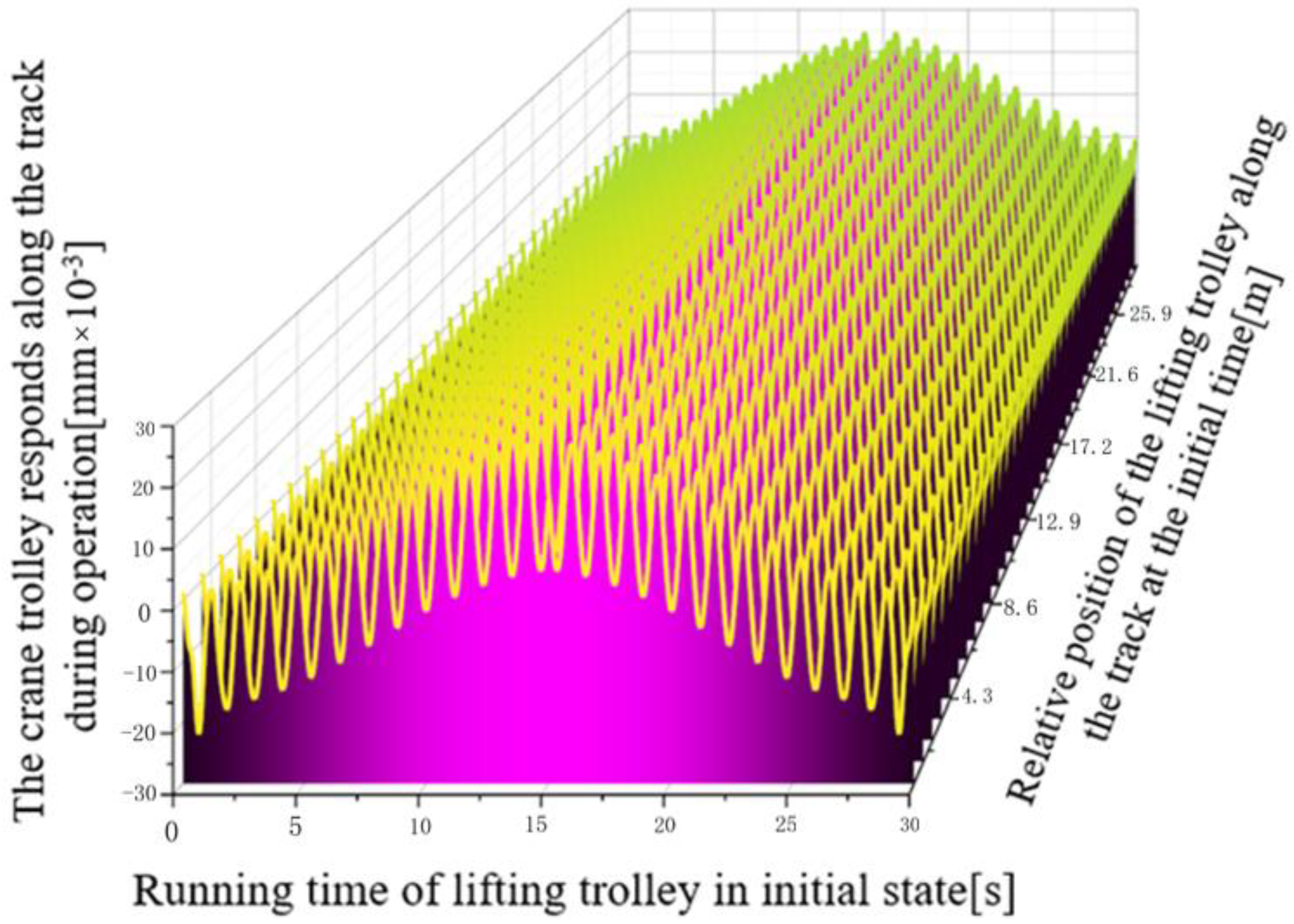
It can be seen from Figure 7 that the response caused by the trolley at both ends of the track is relatively small when the container is being hoisted. As the car approaches the middle section, the response gradually increases to the maximum. The result of this part is affected by the beam section and other factors, and the response caused by other systems is at the minimum value.

Figure 7.
Response of track beam section caused by trolley movement.
Next, the swing of the container caused by the movement of the lifting trolley is analyzed. The response to the twisting and lifting motion of the rope has been analyzed previously. The author assumes here that the lifting rope can be equivalent to a rope from the bottom centroid of the trolley to the top centroid of the container. It has two degrees of freedom as shown in Figure 8, respectively, the movement of the car along the track and the swing of the container . The first Lagrange equation with redundant coordinates is used here to establish the dynamics equation.
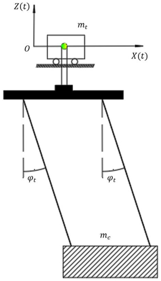
Figure 8.
Simplified diagram of container swing.
Bring the last two equations into the Lagrange equation.
and in the above formula represent Lagrange redundancy factors with redundancy parameters. represents the swing angle of the container perpendicular to the track plane when the crane trolley is moving.
According to the above equations, the relationship between the container swing angle and the swing amplitude along the carriage movement direction is obtained.
The position of the container in the process of car driving is represented by coordinates. Depending on the conditions, the container is swung by the rope under the drive of the trolley. This part of the response can be broken down into a response along the x direction and a response along the z direction.
indicates the power of the driving motor of the lifting trolley. represents the speed of the trolley in its initial state.
The external excitation of a 4-DOF container crane in trolley motion is listed above. The responses of the moving direction of the trolley and the moving direction of the lifting wire rope are solved, respectively.
and represent the response of the lifting trolley moving in the x direction and the response of the container swinging angle changing to the x direction, respectively. indicates the vertical response caused by the container swing angle. and indicate the start and end time of the trolley movement.
The first two equations correspond to the response of the first and second terms of the excitation applied with the car dynamics equation in the direction, respectively. As can be seen from Figure 9 and Figure 10, the movement of the lifting trolley in the initial state has a large impact on the response of the container at the beginning and end. Due to the influence of the span of the trolley, when the movement is furthest away from the initial orbit, the response will gradually become flat.
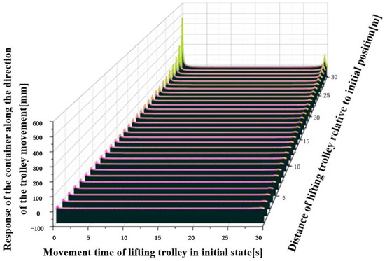
Figure 9.
Lateral response of container caused by movement of lifting trolley.
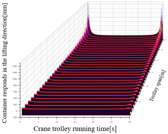
Figure 10.
Container response along the lifting direction caused by the movement of the lifting trolley.
2.4. The Response Caused by the Crane Operating Mechanism in the System Setting State
The response of the port container crane under the initial state excitation is solved. The container is first connected by ropes, lifting carts, then rails, and finally, to the cart. The influence of transverse bending vibration of the beam on the container is not considered. When the cart is moving, the response of the container at this moment can be broken down into a swing along the cart direction and perpendicular to the plane. The establishment of the dynamic equation and the solution of the response are similar to that part when the car is moving.
indicates the power of the motor driven by the crane. represents the speed of the crane in its initial state.
The response of the container when the truck is running is the following expression.
and represent the response of the crane moving in the y direction and the response of the container swing angle changing in the y direction, respectively. indicates the vertical response caused by the container swing angle. and indicate the start and end times of the crane movement.
As can be seen from Figure 11 and Figure 12, when the crane is running according to the initial state, the response of the container will have a relatively obvious change at the initial moment. After several spikes, it gradually flattens out. Moreover, affected by the position of the car in the track, this response change is most obvious when the car runs to the furthest distance from the initial position.
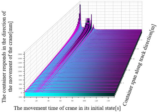
Figure 11.
Response of the container along the direction of the trolley track caused by the movement of the crane.
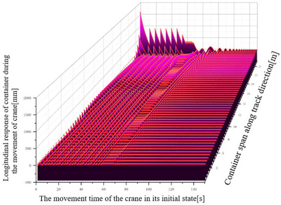
Figure 12.
Response of the container along the lifting direction caused by the movement of the crane.
3. The Proposed Method of SPE Stability Control for Multi-Degree-of-Freedom System under Specific Conditions
First, the authors describe the basic principles of SPE methods. We finds that it is necessary to determine the specific time and excitation amplitude to control the actual system according to the traditional mechanical control theory. The responses of spatial four-degree-of-freedom systems in specific states have been solved previously. It is found that the amplitude of container swing is too large in some states, so it is proposed to control the excitation under the setting range of swing amplitude. This is known as the specific point in time excitation (SPE) method. The principle of this method is that in the equation of state determining the motion of the system, when the response is found to be too large, the external excitation intervenes in advance. With the control of the driving motor, the amplitude of the container swing is reduced to the specified range. This method first needs to decompose the motion state of the whole system at different times, and then determine the moment and the size of the excitation. The basic principle is expressed as the following equation.
The first item at the right end of the above formula is the excitation of the system in the initial state. The second is the external excitation for controlling the drive motor of each mechanism after the swing amplitude of the container exceeds the range of the system. The response generated by this excitation is superimposed on the response in the initial state. Finally, the overall response is reduced to a reasonable range.
stands for initial excitation force. indicates the power of the motor driving the specified system. and represent the interval of velocity variation of SPE intervention. and indicate the time interval for SPE intervention.
The response of four mechanisms of container crane systems under the action of SPE is solved. In the order driven by the system, time is brought in as a one-dimensional function. Firstly, the response of the lifting mechanism under the action of SPE is solved.
and represent the speed range of the lifting mechanism under the action of SPE. and represent the time interval of the lifting mechanism under SPE action. indicates the operating time of the lifting mechanism system.
The first term of the above integral represents the range of changes in a certain period of time when the lifting system is transformed into an external excitation. The delta function is a generalized function, which means that the expression has the right to be assigned within the specified time period, and the result that is not in the integration time period is assigned to zero.
According to the order of work, the lifting mechanism can be operated shortly before the rotating device can work. The rotating device can adjust the rotational speed during rotation according to the requirements of product design. Based on this, the response of the rotating device under the action of SPE is obtained.
and represent the range of speed variation of the rotating device. and represent the time interval in which the rotating device is under SPE action. indicates the working time of the rotating device. indicates the distance from the connection between the rope and the drum to the center of the container.
During the intervention of the rotating device into the SPE, the sum function that appears above is related to the fourth order frequency of the previous rotating device in its initial state.
The response of the whole system car driven by SPE is solved below. Different from the previous solution, the movement of the container can be decomposed into the change of amplitude along the track direction and the swing of the container with the rope around the trolley when the trolley speed changes. A change in the swing angle is ultimately equivalent to a change in the amplitude in the x and z directions.
and represent the speed range of the lifting trolley under the action of SPE. and represent the time interval of the lifting trolley under SPE intervention. represents the working time of the lifting trolley system.
After analysis, the longitudinal response of the sudden change in speed of the crane trolley to the track is the same as that under the initial state excitation, so the analysis is no longer carried out. Finally, the response of the container crane under SPE is analyzed. Similar to the response produced by the car, the difference is that the external excitation is in a different time interval.
and represent the speed range of the lifting truck under the action of SPE. and represent the time interval of the lifting cart under SPE intervention. indicates the working time of the crane system.
In this way, the response of a four-degree-of-freedom container gantry crane under SPE action is solved. It should be noted that the time interval in which SPE is applied to each part of the device is always within the time interval in which excitation is applied to that direction in the initial state. The SPE intervenes only if the container swings along the space beyond the specified distance at a certain height.
4. Stability Verification of Container Crane System under the Action of SPE
4.1. Dynamic Simulation Results of Container Gantry Crane Model under SPE Action
The authors set that when the swing amplitude of the container exceeds 5 cm in the x and y directions and 3 cm in the z direction, the SPE will start to intervene. When the pack swings less than 3 cm in all directions, the SPE stops working. At this time, the excitation of the container remains fixed until the operation ends at the specified position.
In order to make the simulation result closer to the actual working condition, the author takes the maximum distance of the actual container to carry out dynamic simulation. The lifting system for the container gantry crane is set up first. After 5 s, the device is turned the to work. The lifting car and the lifting truck begin to work at the same time. The working time of the lifting system is 105 s. The operation time of the rotating device is 30 s. The crane trolley operates for 30 s. The crane works for 150 s. In the dynamic simulation, the response data of the container along the lifting direction and the moving direction of the lifting trolley are recorded, respectively. Finally, these data are drawn into contouring colors to fill the image. Figure 13, Figure 14 and Figure 15 are the dynamic simulation results of the container gantry crane model under the action of SPE. As can be seen from Figure 13, when the container lifting system is working, the longitudinal response has a large amplitude. With the intervention of SPE, the amplitude decreases significantly in a short period of time. The work of the rotating device and the lifting trolley cause the container to change amplitude again, but this time, the role of the SPE is more obvious. At about 20 s of system operation, the response of the container is already lower than the first amplitude, and soon it flattens out. The overall structure is less affected by the track position of the lifting trolley. Figure 14 illustrates the response of the container along the direction of carriage movement under the action of the SPE. When the trolley is moving, the amplitude of the container quickly reaches its maximum, and the intervention of the SPE causes the amplitude to drop rapidly within a few seconds. The dynamic simulation data images show that the SPE action time is timely and effective. Figure 15 shows the dynamic simulation data of container response of the lifting truck under the action of SPE. At this time, the response of the container along the direction of the movement of the crane quickly peaks with the movement of the crane in a short period of time. The intervention of SPE not only reduces the amplitude of the container response rapidly, but also the response after the action is lower than the amplitude before the lifting truck has not moved. It is more effective to prove the effectiveness of SPE.
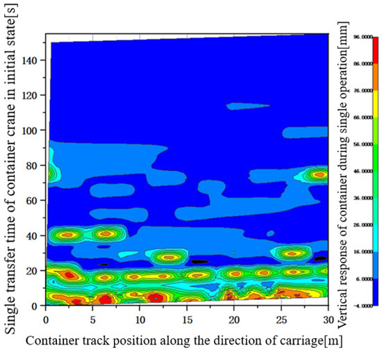
Figure 13.
Response of the container centroid position along the lifting direction under the action of the SPE.
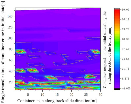
Figure 14.
Response of the container centroid position along the moving direction of the trolley under the action of the SPE.
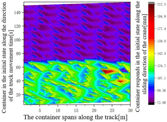
Figure 15.
Response of the container centroid position along the direction of the crane movement under the action of SPE.
When the container swings in three directions beyond the control range, the SPE intervenes in time to smooth it out in a short time. And in the second half of the operation period, the overall swing amplitude is always maintained at a low level. It shows that the intervention of SPE has a good control effect.
4.2. Numerical Results of Container Gantry Crane under SPE Action
To verify the validity of dynamic model simulation results under the action of SPE, the numerical model verification results under SPE are added in this paper. At the same time, the container response data will be expanded according to four subsystems according to the modeling method of the numerical model. In dynamic simulation, because it is difficult to accurately extract the rotational response angle of the container, it is equivalent to the response of the container along the Cartesian coordinate system. However, it is still easy to extract the exact numerical results, and it is only necessary to convert the angular response of the container in the numerical results into the response of the container along the direction of the lifting trolley and along the lifting truck in the dynamic results.
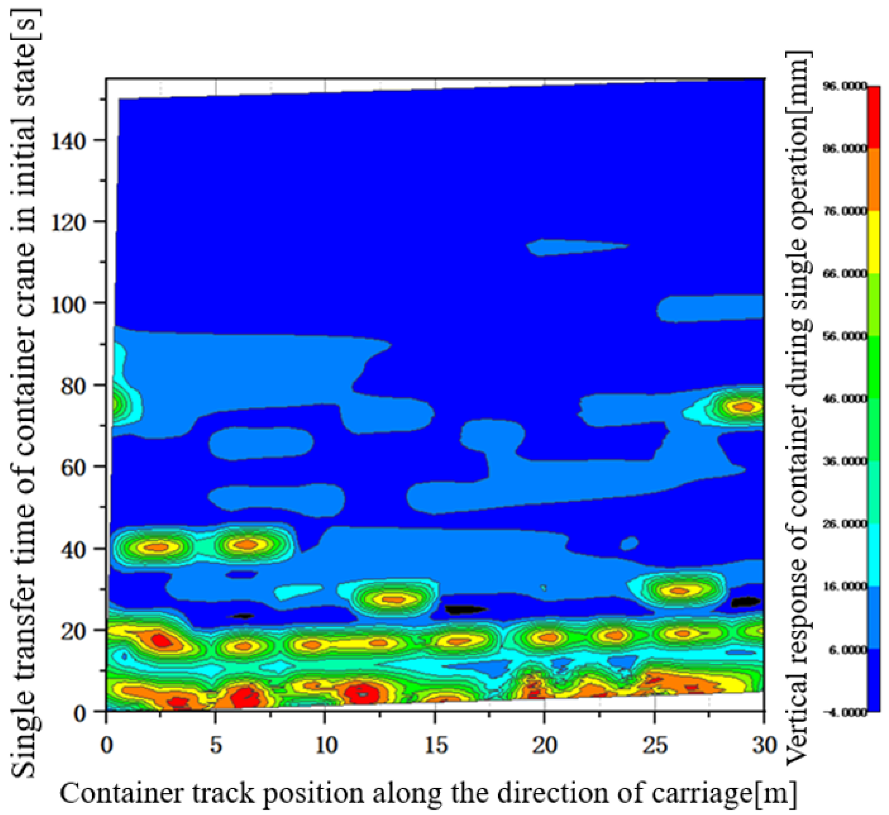
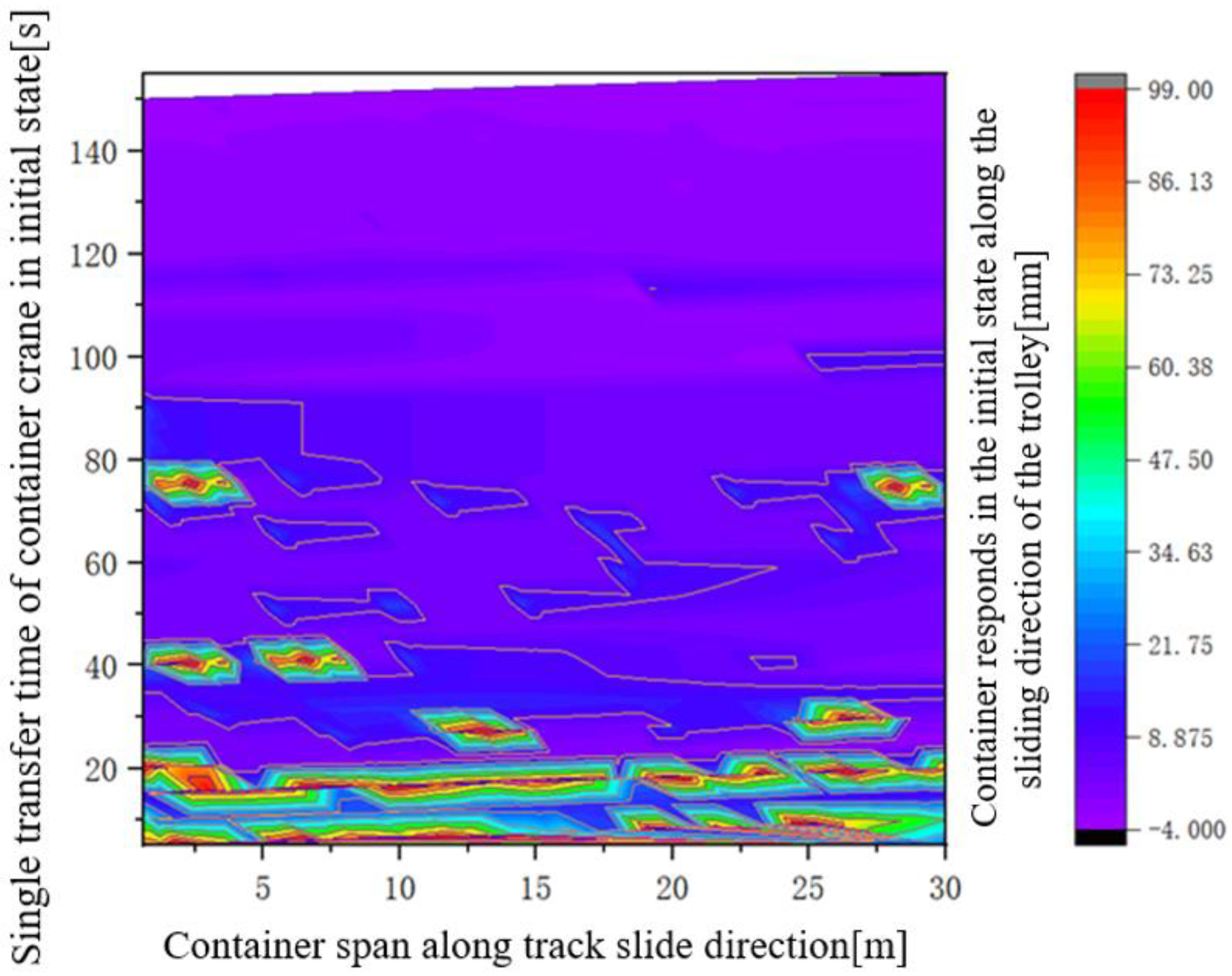
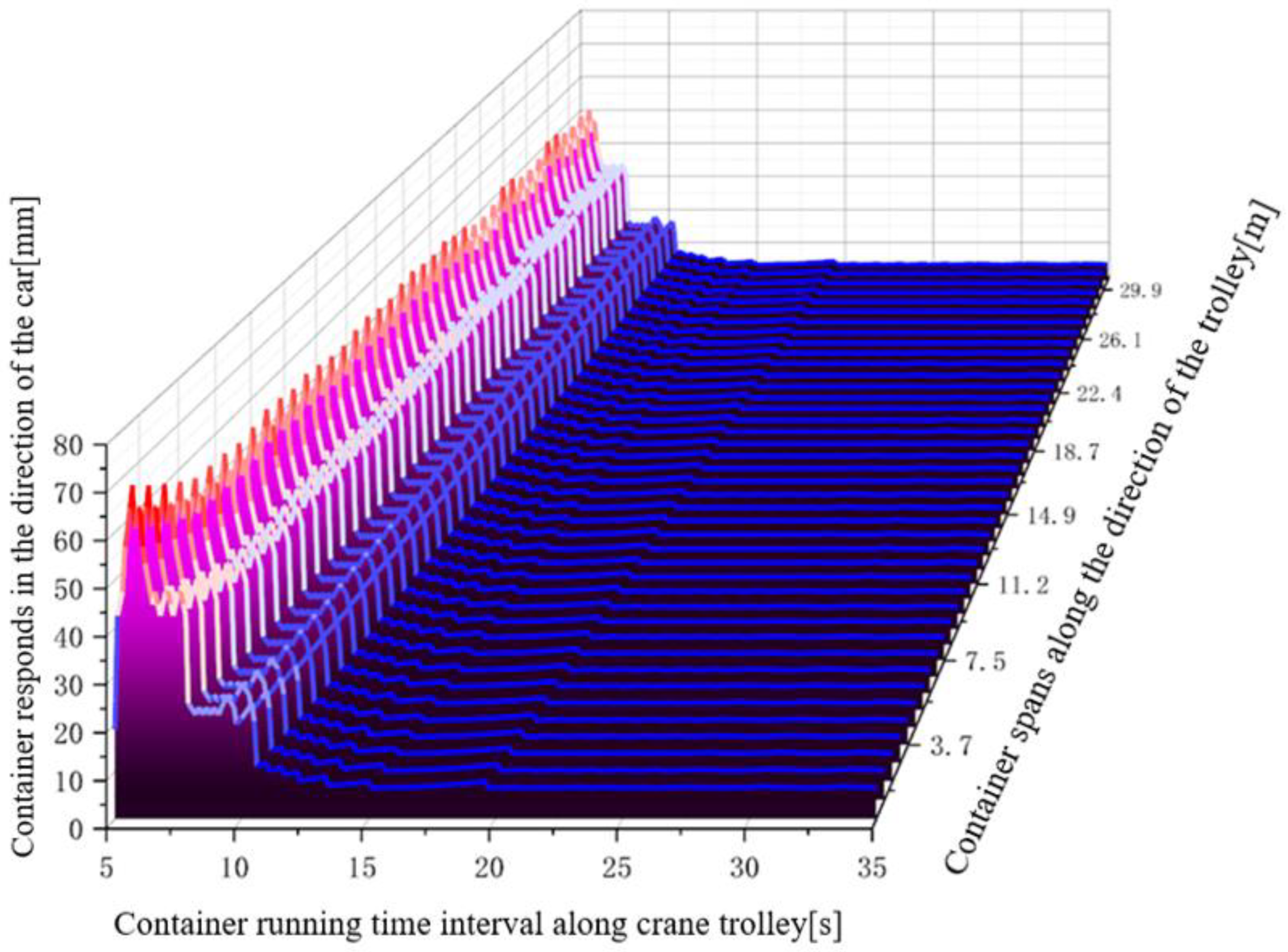
Figure 16, Figure 17, Figure 18 and Figure 19 are the numerical results of the container gantry crane under the action of SPE. Compared with the previous dynamic simulation results, Figure 16 illustrates the container swing amplitude of the numerical model, which can maintain the stability of the container for only a short time under the action of SPE. Moreover, the effect of SPE intervention is more pronounced in the second half of the rotating device operating period. Figure 17 is a control diagram of the container response of the lifting system under the action of SPE. It can be seen that two peaks have been experienced, because during the operating time interval of the lifting system, the lifting trolley and the truck also start to work according to the setting of the system. The effect of SPE intervention is very obvious, mainly in the last two-thirds of the hoisting system. During this period, the vertical response data of the container meet control standards and tend to be stable. Figure 18 and Figure 19, respectively, show the response images of the container numerical model of the lifting trolley and the big truck under SPE intervention. Both charts show a spike. The difference is that the response image of the container shows that the lifting trolley experienced about 10 s of container swing to reach the set control standard with SPE intervention, and the lifting truck took about 30 s. The numerical results of the four subsystems all show that in the second half of the working time, the swing amplitude of the container is in line with the control standard, which forms a good verification relationship with the dynamic simulation image. At the same time, the timeliness and effectiveness of the SPE method are proven.
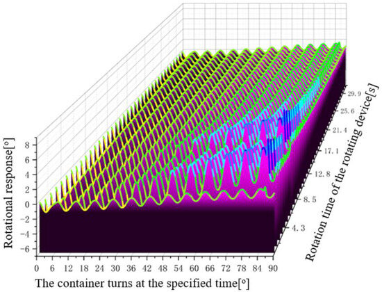
Figure 16.
Numerical response of container in rotation direction under SPE action.
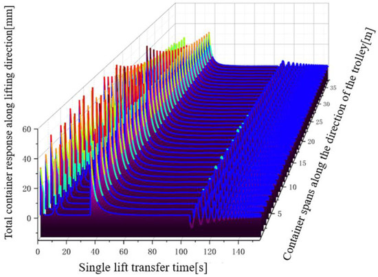
Figure 17.
Numerical response of container in lifting direction under SPE action.

Figure 18.
Numerical response of the container along the direction of car movement under the action of SPE.
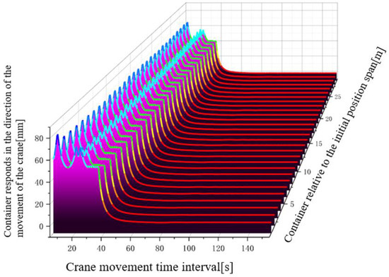
Figure 19.
Numerical response of the container along the direction of the truck movement under the action of SPE.
The response amplitude of numerical simulation is lower than that of dynamic simulation. The data image of the dynamic simulation shows that the overall SPE intervention time is a few seconds later than the numerical response intervention time. This may be caused by the uneven structure and quality of the container gantry crane. The similarity is that the response amplitude of the whole system will decrease significantly when SPE is involved in both numerical simulation and model dynamic simulation. The final numerical and dynamic simulation results prove that the SPE method has a good stability control effect on container gantry cranes.
5. Conclusions and Prospects
In this paper, the authors take the four-degree-of-freedom container gantry crane system as the research object. The stability control method of SPE is presented for the first time. The effectiveness of this method is proven with experiments. The main contribution of the authors is to decouple the motion of a spatial four-degree-of-freedom system. The container response is solved efficiently and precisely using a one-dimensional wave equation, the Lagrange dynamic equation, Fourier transform, and other methods. The experiment proves that these methods have a good control effect on the swing of the container. The expected experimental goal was achieved.
The most obvious effect of SPE is that the operating time of the container’s four subsystems is set to whatever standard. As long as the SPE is involved in time, the swing amplitude of the container will always meet the set standard in the first half of the corresponding time interval. Even in the first third of the operation of the trolley and the truck with a long relative operation time, the swing amplitude of the container has met the set standard. This is very important both from the point of view of safety and from the point of view of the efficiency of container logistics in ports. The dynamic simulation results of the physical model and the simulation of the numerical model prove this.
The SPE method can be used in the future for container transfer in unmanned smart ports. It should be pointed out that this method can no longer rely on the feedback of real-time swing data during container operation to a certain extent, and it is an active control system. Inevitably, environmental factors such as sudden changes in wind and earthquakes need to be taken into account. In order to achieve this control effect, it may be necessary to collect relevant data in the field and pass relevant data to the SPE control system prior to operation. For example, if the possible effects of external forces (wind) need to be added, the wind level needs to be converted into the form of excitation into the SPE model before a single container run. The proposed SPE method provides a new experimental scheme for future smart logistics ports and is expected to play its due role.
Author Contributions
Conceptualization, S.Z. and Y.Q.; methodology, S.Z.; software, S.Z.; validation, S.Z. and Y.Q.; formal analysis, S.Z.; investigation, S.Z.; resources, S.Z.; data curation, S.Z.; writing—original draft preparation, S.Z.; writing—review and editing, S.Z.; visualization, S.Z.; supervision, Y.Q.; project administration, Y.Q.; funding acquisition, Y.Q. All authors have read and agreed to the published version of the manuscript.
Funding
This work was supported by the Shanxi Provincial Key Research and Development Project (201903D121067) and the Fund for Shanxi ‘1331’ Project’ Key Subjects Construction (1331KSC).
Data Availability Statement
The data that support the findings of this study are available from the corresponding author, [author initials], upon reasonable request.
Conflicts of Interest
The authors declare no conflict of interest.
Appendix A
The analytical solution of the angle and torque of the connection between the wire rope and the drum in the rotating system under the system setting state.
Appendix B
Analysis of the transfer matrix elements of the mechanical action on the track beam section of the crane trolley in motion.
References
- Pham, T.Y. A smart port development: Systematic literature and bibliometric analysis. Asian J. Shipp. Logist. 2023, 39, 57–62. [Google Scholar] [CrossRef]
- Zhang, Y. Analysis of Intelligent Logistics and Supply Chain Management Reform in the Digital Era. Sci. Soc. Res. 2023, 5, 18–22. [Google Scholar] [CrossRef]
- Benkert, J.; Maack, R.; Meisen, T. Chances and Challenges: Transformation from a Laser-Based to a Camera-Based Container Crane Automation System. J. Mar. Sci. Eng. 2023, 11, 1718. [Google Scholar] [CrossRef]
- Donta, P.K.; Sedlak, B.; Casamayor Pujol, V.; Dustdar, S. Governance and sustainability of distributed continuum systems: A big data approach. J. Big Data 2023, 10, 53. [Google Scholar] [CrossRef]
- Casamayor Pujol, V.; Morichetta, A.; Murturi, I.; Kumar Donta, P.; Dustdar, S. Fundamental Research Challenges for Distributed Computing Continuum Systems. Information 2023, 14, 198. [Google Scholar] [CrossRef]
- Wang, T.; Zhou, J.; Wu, Z.; Liu, R.; Zhang, J.; Liang, Y. A Time-Varying PD Sliding Mode Control Method for the Container Crane Based on a Radial-Spring Damper. Electronics 2022, 11, 3543. [Google Scholar] [CrossRef]
- Yin, Y.; Tao, Y.; Wang, C. Relatively maximal perturbation bounds for global robustness of max-plus linear systems. Int. J. Robust Nonlinear Control 2021, 31, 4170–4183. [Google Scholar] [CrossRef]
- Ngo, Q.H.; Nguyen, N.P.; Truong, Q.B.; Kim, G.-H. Application of Fuzzy Moving Sliding Surface Approach for Container Cranes. Int. J. Control Autom. Syst. 2020, 19, 1133–1138. [Google Scholar] [CrossRef]
- Ngo, Q.H.; Nguyen, N.P.; Nguyen, C.N.; Tran, T.H.; Bui, V.H. Payload pendulation and position control systems for an offshore container crane with adaptive-gain sliding mode control. Asian J. Control 2020, 22, 2119–2128. [Google Scholar] [CrossRef]
- Yu, Z.; Dong, H.M.; Liu, C.M. Research on Swing Model and Fuzzy Anti Swing Control Technology of Bridge Crane. Machines 2023, 11, 579. [Google Scholar] [CrossRef]
- Fasih ur Rehman, S.M.; Mohamed, Z.; Husain, A.R.; Jaafar, H.I.; Shaheed, M.H.; Abbasi, M.A. Input shaping with an adaptive scheme for swing control of an underactuated tower crane under payload hoisting and mass variations. Mech. Syst. Signal Process. 2022, 175, 109106. [Google Scholar] [CrossRef]
- Xin, X.; Makino, K.; Izumi, S.; Yamasaki, T.; Liu, Y. Anti-Swing control of the Pendubot using damper and spring with positive or negative stiffness. Int. J. Robust Nonlinear Control 2021, 31, 4227–4246. [Google Scholar] [CrossRef]
- Susanto, E.; Wibowo, A.S.; Rachman, E.G. Fuzzy Swing Up Control and Optimal State Feedback Stabilization for Self-Erecting Inverted Pendulum. IEEE Access 2020, 8, 6496–6504. [Google Scholar] [CrossRef]
- Li, H.; Hui, Y.B.; Wang, Q.; Wang, H.X.; Wang, L.J. Design of Anti-Swing PID Controller for Bridge Crane Based on PSO and SA Algorithm. Electronics 2022, 11, 3143. [Google Scholar] [CrossRef]
- Guo, Q.; Chai, L.; Liu, H. Anti-swing sliding mode control of three-dimensional double pendulum overhead cranes based on extended state observer. Nonlinear Dyn. 2022, 111, 391–410. [Google Scholar] [CrossRef]
- Sun, Z.; Ling, Y.; Tan, X.; Zhou, Y.; Sun, Z. Designing and application of type-2 fuzzy PID control for overhead crane systems. Int. J. Intell. Robot. Appl. 2021, 5, 10–22. [Google Scholar] [CrossRef]
- Wu, Q.; Wang, X.; Hua, L.; Xia, M. Modeling and nonlinear sliding mode controls of double pendulum cranes considering distributed mass beams, varying roped length and external disturbances. Mech. Syst. Signal Process. 2021, 158, 107756. [Google Scholar] [CrossRef]
- Wu, Q.; Wang, X.; Hua, L.; Xia, M. Improved time optimal anti-swing control system based on low-pass filter for double pendulum crane system with distributed mass beam. Mech. Syst. Signal Process. 2021, 151, 107444. [Google Scholar] [CrossRef]
- Miranda-Colorado, R. Robust observer-based anti-swing control of 2D-crane systems with load hoisting-lowering. Nonlinear Dyn. 2021, 104, 3581–3596. [Google Scholar] [CrossRef]
- Ramli, L.; Mohamed, Z.; Efe, M.; Lazim, I.M.; Jaafar, H. Efficient swing control of an overhead crane with simultaneous payload hoisting and external disturbances. Mech. Syst. Signal Process. 2020, 135, 106326. [Google Scholar] [CrossRef]
- Tian, Z.; Yu, L.; Ouyang, H.; Zhang, G. Swing suppression control in tower cranes with time-varying rope length using real-time modified trajectory planning. Autom. Constr. 2021, 132, 103954. [Google Scholar] [CrossRef]
- Hu, D.; Qian, Y.; Fang, Y.; Chen, Y. Modeling and nonlinear energy-based anti-swing control of underactuated dual ship-mounted crane systems. Nonlinear Dyn. 2021, 106, 323–338. [Google Scholar] [CrossRef]
- Jensen, K.J.; Ebbesen, M.K.; Hansen, M.R. Anti-swing control of a hydraulic loader crane with a hanging load. Mechatronics 2021, 77, 102599. [Google Scholar] [CrossRef]
- Li, C.; Xia, Y.; Wang, W. H-infinity Output-Feedback Anti-Swing Control for a Nonlinear Overhead Crane System with Disturbances Based on T-S Fuzzy Model. IEEE Access 2021, 9, 135571–135584. [Google Scholar] [CrossRef]
- Meisuh, B.K.; Huh, J.; Haldar, A.; Kim, I.T. Comparison of seismic responses of a jumbo-size container crane retrofitted with braces, dampers, and isolation systems. Ocean Eng. 2022, 262, 112222. [Google Scholar] [CrossRef]
- Meisuh, B.K.; Seo, J.; Huh, J.; Kim, J.; Kim, J.M. Seismic response of a container crane subjected to ground motions. Appl. Ocean Res. 2022, 126, 103270. [Google Scholar] [CrossRef]
- Nguyen, V.B.; Huh, J.; Meisuh, B.K.; Tran, Q.H. Shake table testing for the seismic response of a container crane with uplift and derailment. Appl. Ocean Res. 2021, 114, 102811. [Google Scholar] [CrossRef]
- Su, N.; Peng, S.; Hong, N. Stochastic dynamic transient gusty wind effect on the sliding and overturning of quayside container cranes. Struct. Infrastruct. Eng. 2021, 17, 1271–1283. [Google Scholar] [CrossRef]
- Zhou, Y.; Fu, Z.; Zhang, J.; Li, W.; Gao, C. A Digital Twin-Based Operation Status Monitoring System for Port Cranes. Sensors 2022, 22, 3216. [Google Scholar] [CrossRef] [PubMed]
- Tong, M.; Shen, Y. Research on coupled vibration of wheel–rail beam system in the high-speed quayside container crane. Mech. Adv. Mater. Struct. 2020, 27, 1473–1482. [Google Scholar] [CrossRef]
- Li, W.; Quan, L.; Hu, X.; Men, X. A comprehensive framework for model validation and reliability assessment of container crane structures. Struct. Multidiscip. Optim. 2020, 62, 2817–2832. [Google Scholar] [CrossRef]
- Kim, G.-H. Continuous Integral Sliding Mode Control of an Offshore Container Crane with Input Saturation. Int. J. Control Autom. Syst. 2020, 18, 2326–2336. [Google Scholar] [CrossRef]
- Fasih ur Rehman, S.M.; Mohamed, Z.; Husain, A.R.; Ramli, L.; Abbasi, M.A.; Anjum, W.; Shaheed, M.H. Adaptive input shaper for payload swing control of a 5-DOF tower crane with parameter uncertainties and obstacle avoidance. Autom. Constr. 2023, 154, 104963. [Google Scholar] [CrossRef]
- La, V.D.; Nguyen, K.T. Combination of input shaping and radial spring-damper to reduce tridirectional vibration of crane payload. Mech. Syst. Signal Process. 2019, 116, 310–321. [Google Scholar] [CrossRef]
- Hamza, M.F.; Yap, H.J.; Choudhury, I.A.; Isa, A.I.; Zimit, A.Y.; Kumbasar, T. Current development on using Rotary Inverted Pendulum as a benchmark for testing linear and nonlinear control algorithms. Mech. Syst. Signal Process. 2019, 116, 347–369. [Google Scholar] [CrossRef]
- Sun, M.; Wang, S.; Han, G.; An, L.; Chen, H.; Sun, Y. Modeling and Dynamic Analysis of a Triple-Tagline Anti-Swing System for Marine Cranes in an Offshore Environment. J. Mar. Sci. Eng. 2022, 10, 1146. [Google Scholar] [CrossRef]
- Lu, B.; Lin, J.; Fang, Y.; Hao, Y.; Cao, H. Online trajectory planning for three-dimensional offshore boom cranes. Autom. Constr. 2022, 140, 104372. [Google Scholar] [CrossRef]
- Li, G.; Ma, X.; Li, Z.; Li, Y. Optimal trajectory planning strategy for underactuated overhead crane with pendulum-sloshing dynamics and full-state constraints. Nonlinear Dyn. 2022, 109, 815–835. [Google Scholar] [CrossRef]
- Wang, S.; Ren, Z.; Jin, G.; Chen, H. Modeling and Analysis of Offshore Crane Retrofitted with Cable-Driven Inverted Tetrahedron Mechanism. IEEE Access 2021, 9, 86132–86143. [Google Scholar] [CrossRef]
- Li, Z.; Ma, X.; Li, Y. Nonlinear partially saturated control of a double pendulum offshore crane based on fractional-order disturbance observer. Autom. Constr. 2022, 137, 104212. [Google Scholar] [CrossRef]
- Shi, H.; Yao, F.; Yuan, Z.; Tong, S.; Tang, Y.; Han, G. Research on nonlinear coupled tracking controller for double pendulum gantry cranes with load hoisting/lowering. Nonlinear Dyn. 2022, 108, 223–238. [Google Scholar] [CrossRef]


Disclaimer/Publisher’s Note: The statements, opinions and data contained in all publications are solely those of the individual author(s) and contributor(s) and not of MDPI and/or the editor(s). MDPI and/or the editor(s) disclaim responsibility for any injury to people or property resulting from any ideas, methods, instructions or products referred to in the content. |
© 2023 by the authors. Licensee MDPI, Basel, Switzerland. This article is an open access article distributed under the terms and conditions of the Creative Commons Attribution (CC BY) license (https://creativecommons.org/licenses/by/4.0/).