Abstract
Global routing plays a crucial role in printed circuit board (PCB) design and affects the cost of the design significantly. Conventional methods based on rectangular grids have some limitations, whereas this paper introduces a new algorithm that employs a triangular grid model, which offers a more efficient solution to the problem. Firstly, we present a technique to sort all unconnected two-pin nets. Next, a triangular grid graph is constructed to represent the routing resources on the printed circuit board. Finally, we use the concept of maximum flow to identify the paths for global routing and apply detailed routing for the completion of wires. Results from experiments demonstrate that our algorithm is faster than two state-of-the-art routers and does not have any design rule violations for all industrial PCB instances.
1. Introduction
Printed circuit boards (PCBs) are widely used in various fields due to their small size and light weight. As integrated circuits continue to develop on a larger scale and electronic products require more complex functions, the number of pins on PCBs has significantly increased. Manual design methods alone can no longer meet market demands, leading to the emergence of Electronic Design Automation (EDA). EDA tools efficiently find reasonable solutions for complex circuits, reducing labor and cost while improving design efficiency and production processes, making them popular among many enterprises.
Routing is the most crucial process in PCB design, but it is both time-consuming and challenging. It directly impacts the performance of the entire circuit system and can be divided into two parts: global routing and detailed routing. Global routing plans the approximate routing path for each net, reducing the complexity of the routing problem and laying the foundation for detailed routing. Detailed routing calculates the final routing path based on the results of preliminary global routing planning. The key problems in global routing algorithms are how to reduce algorithm running time and how to improve the utilization of routing space.
1.1. Previous Works
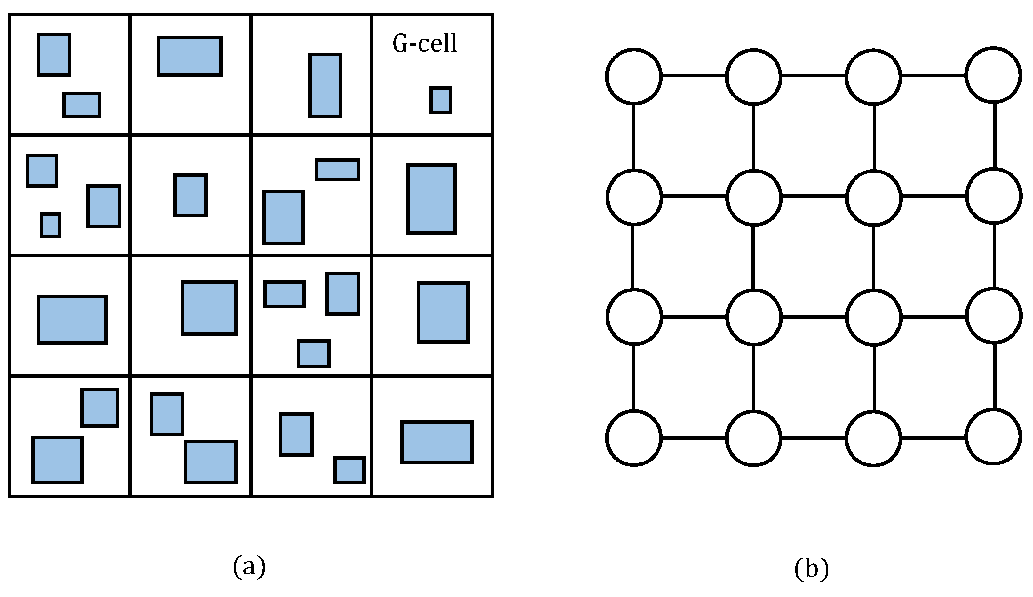
In the field of integrated circuits (ICs), the global routing problem [1] can be modeled as a grid graph , where each vertex corresponds to a rectangular area of the chip, referred to as the global routing cell (G-cell). If G-cell i and G-cell j are adjacent, then we construct an edge , as illustrated in Figure 1. A maximum wiring resource is assigned to each edge . The goal of global routing is to find a path through that connects the pins in G-cells for each net.
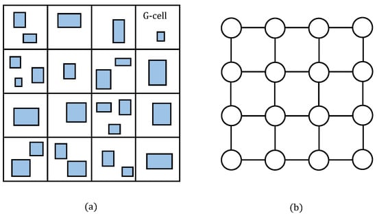
Figure 1.
The construction of grid graph for the global routing problem in IC. (a) Real circuit with G-cells. (b) Grid graph for routing.
In recent years, several high-quality global routers have been developed to solve this problem. FastRoute 4.0 [2] and NTHU-Route 2.0 [3] focus on generating routing paths on a grid graph with a given edge capacity. They employ the ripping-up and rerouting techniques to obtain overflow-minimized solutions. BoxRouter [4] uses a minimum Steiner tree to decompose multi-pin nets into two-pin nets and applies integer programming to find routes for nets in a routing region. VFGR [5] and SPRouter [6] utilize parallelization techniques to handle congestion effectively.
Given that modern integrated circuits and chips frequently comprise multi-layered structures, CUGR [7] operates directly on the 3D grid graph. Conversely, COALA [8] employs a strategy of 2D global routing followed by layer assignment. These approaches cater to the complexities of contemporary IC designs and contribute to the advancement of efficient global routing algorithms.
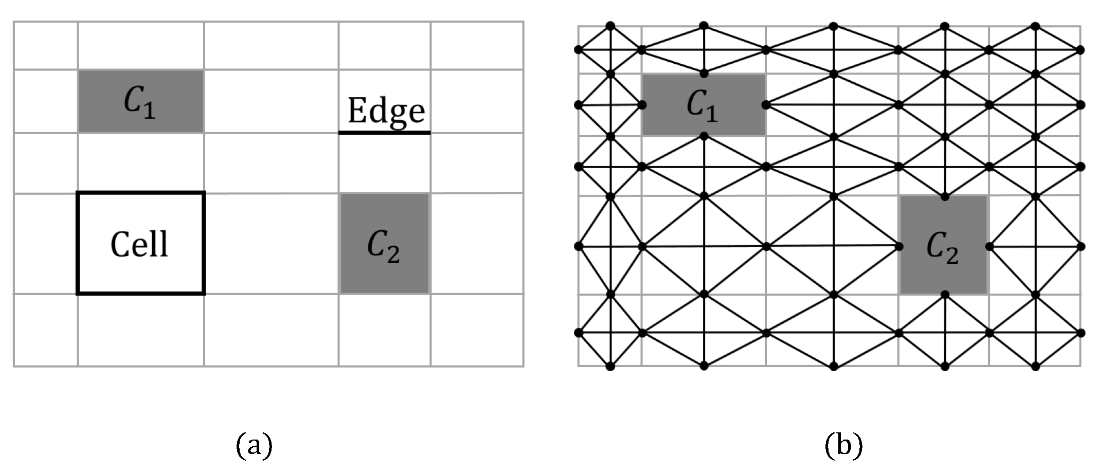
The differences between PCB global routing and integrated circuit global routing are notable. In PCB global routing, initial topological bus routes are created by routing buses on a single layer that encompasses the routing resources of all routing layers. To encompass all routing resources on the circuit board, Wong et al. [9] proposed the utilization of the data structure of the Hanan grid and dynamic routing graph. The Hanan grid is formed from the components by extending their boundaries until they intersect with other components or the board boundaries. Both the board and its components are represented by bounding boxes. The dynamic routing graph features vertices that represent the middle points of all Hanan grid edges, with its edges connecting vertices within the same cell. When an edge is occupied by a bus, the cell is divided into two parts, leading to the creation of new vertices and edges, as illustrated in Figure 2. However, it is worth noting that this method incurs high time and space costs. Processing a few hundred nets can take several tens of minutes. Furthermore, unordered routing may intensify the complexity and impact the routing quality. As a result, Lin et al. [10] proposed a concurrent hierarchical SER method, which incorporates both escape and area routing to compensate for the absence of unordered escape routing.
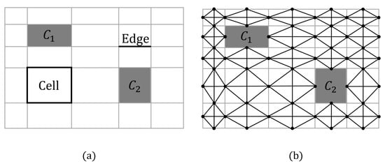
Figure 2.
A schematic diagram of global routing in an example of PCB. (a) The Hanan grid. (b) The dynamic routing graph constructed for the example before routing on the Hanan grid.
In the final phase of the routing process, detailed routing is conducted to establish the specific wires on the board that fulfill the requirements of industrial production based on the outcomes of global routing. During this stage, designers must account for the boundaries of actual obstacles, wire width, spacing between wires and obstacles, and the wire topology. Detailed routing has been the subject of extensive research, including investigations by Yan and Chen [11], who devised length-matching paths for obstacle-aware bus routing. Ozdal et al. [12,13] used a Lagrangian relaxation (LR) framework to allocate extra routing resources around nets simultaneously. Kim et al. [14] introduced a compact topology-aware bus routing approach capable of synthesizing the routing topology of the bus while minimizing design rule violations in designs with high bus density and track utilization. Chen et al. [15] proposed a maze routing method to address non-uniform track resources using a concurrent and hierarchical scheme for buses, whereas Hsu et al. [16] applied a directed acyclic graph (DAG)-based algorithm to connect buses and alleviate routing congestion through rip-up and rerouting. Additionally, Zhang et al. [17] introduced the concept of topological Boolean satisfiability to verify the legality of a segment during the detailed routing stage and determine the existence of feasible bit ordering. Finally, Merrill et al. [18] put forward a novel algorithm capable of managing multiple real-world, intricate constraints such as differential-pair couple routing constraints, pad entry constraints, and more to facilitate printed circuit board routing and generate high-quality, manufacturable layouts.
1.2. Our Contributions
In response to the 135-degree routing requirements of PCBs, the efficiency of routing methods based on rectangular grid graphs, including Hanan graphs, needs to be further improved. Therefore, we propose an efficient global routing method based on triangular construction. The main contributions of this paper are summarized as follows:
- A new global routing algorithm for PCB is proposed. It does not use the conventional rectangular grid but uses the triangular grid data structure to obtain all the routing resources on the circuit board.
- We propose a decomposition ordering algorithm which prioritizes the connection between important components and nets to reduce the degree of local congestion, and we obtain a better global routing result.
- We put forward the idea of using the maximum flow to find the path and increase the speed of searching.
- Experimental results show that our algorithm has excellent performance in running speed and routing result, while the other two state-of-the-art routers spend more time and violate some constraints.
The remainder of this paper is organized as follows. Section 2 introduces some related terms and routing design rules for PCBs and formulates the addressed problem. Section 3 details the core techniques of our algorithm. Experimental results are shown in Section 4. Finally, Section 5 concludes our work.
2. Preliminaries
In this section, we introduce the basics of the maximum flow model, provide the formal definition of the PCB global routing problem, and explain the relevant terms and routing design rules associated with our problem.
2.1. Maximum Flow Model
Our problem involves a directed graph , where each edge has a non-negative capacity . There is only one source point and one sink point , with other vertices on a path between and , which is referred to as a flow network. The flow from vertex to vertex is denoted by . The objective of the maximum flow problem is to find a flow that maximizes its value, , and satisfies the following conditions [19]:
Let be a path from to . A forward arc is in the same direction as the path and a backward arc is in the opposite direction to the path. If satisfies [19]:
it is called an augmenting path. Given a cut set , the sum of is called the capacity of this cut set, i.e.,
and . In the flow network G, if is a maximal flow, then there is no augmenting path with respect to it, and the value of the flow starting with and ending with is equal to the capacity of the minimal cut set separating and . According to this theorem, the Ford–Fulkerson algorithm [19] is a well-known iterative algorithm to solve the max-flow problem, which is a special linear programming problem, and it is an iterative method. In the beginning, for all , that is, the value of the flows in the network are 0 in the initial state. In each iteration, the flow value can be increased by finding an augmenting path, along which more flows can be pressed. This process is repeated until all the augmenting paths are found.
2.2. Routing Design Rules
In this paper, we aim to simplify the design process while ensuring better manufacturability. To achieve this, our algorithm must accommodate multiple routing design rules. Our problem involves four major design rules, which are detailed below:
- Non-crossing constraint: Net crossing is not permitted on the same layer.
- Wire width and spacing constraint: Each wire has its own width, and there are specific spacing requirements that must be adhered to between wires, obstacles and other elements.
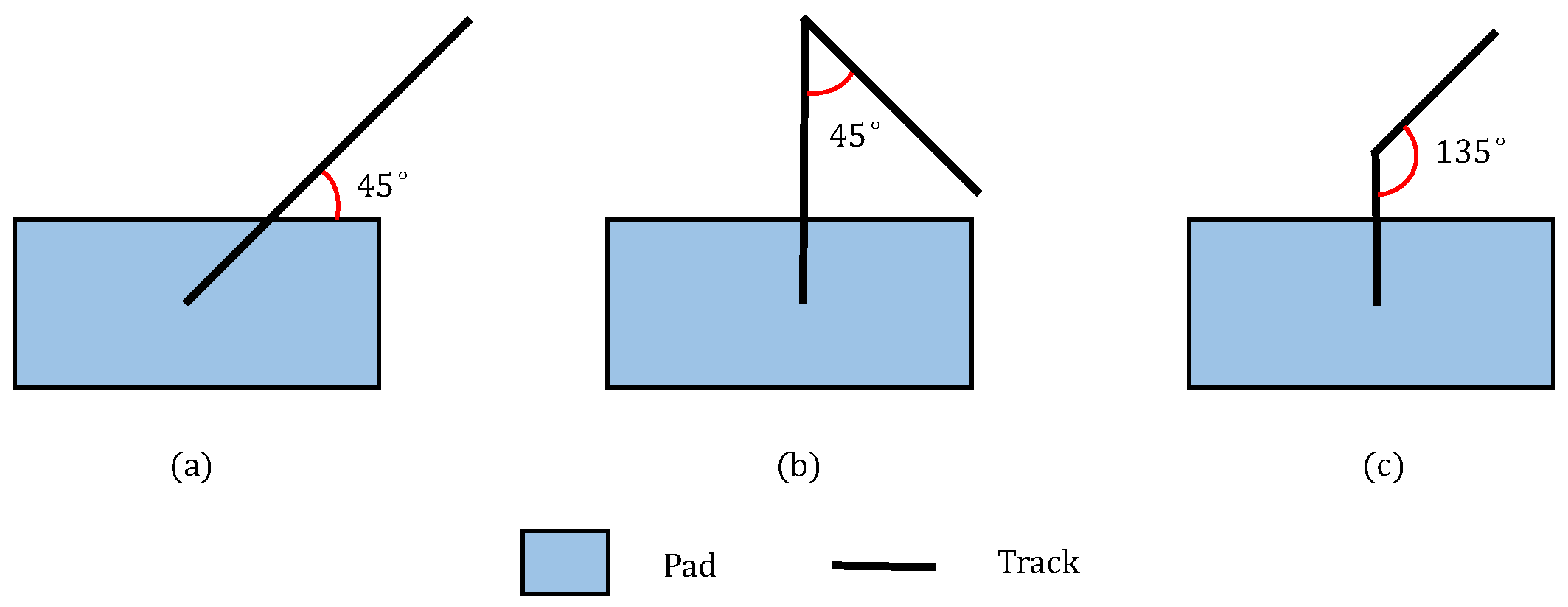
- Routing angle constraint: Our algorithm allows for routing angles of 135 degrees between two tracks, while routing angles of 45 degrees are prohibited. Additionally, routed nets entering a pad must not introduce an acute angle between each other (see Figure 3).
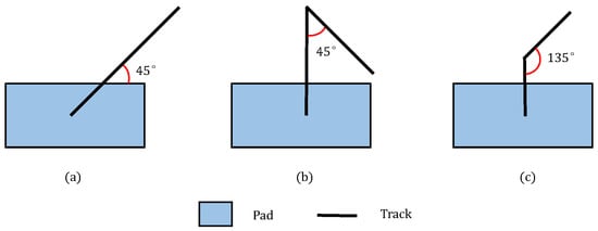 Figure 3. Three cases of the routing angle. (a) Routed nets entering a pad introduce an acute angle between each other. (b) Routing angles of between two tracks. (c) Routing angles of between two tracks. (a,b) are not allowed.
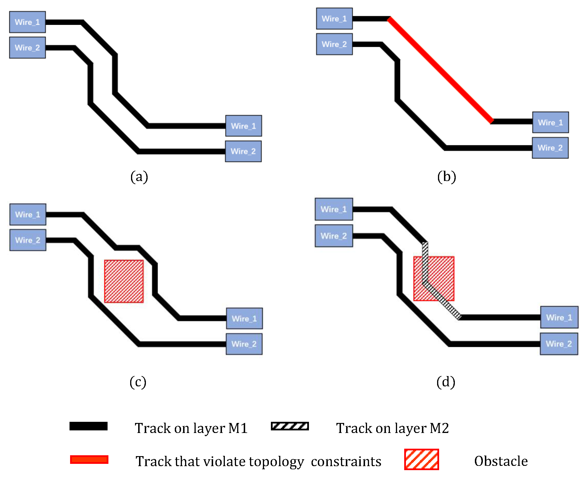
 - Topology matching constraint: Multiple wires should try to meet the same topology structure. This involves four considerations: (1) they should have the same number of segments, (2) they should go through the same layer, (3) they should be routed in the same direction, and (4) the order of each segment should be the same or opposite to the starting order. Topology failures are illustrated in Figure 4.
 Figure 4. Four examples of topology. (a) Perfect topology. (b) Bad topology. (c) Topology allowed when avoiding obstacle. (d) Topology forbidden when avoiding obstacle.
2.3. Problem Formulation
Given a set of items such as pads, vias, tracks, a netlist N, and routing design rules, we connect all the nets so that there are no design rule violations.
3. Algorithms
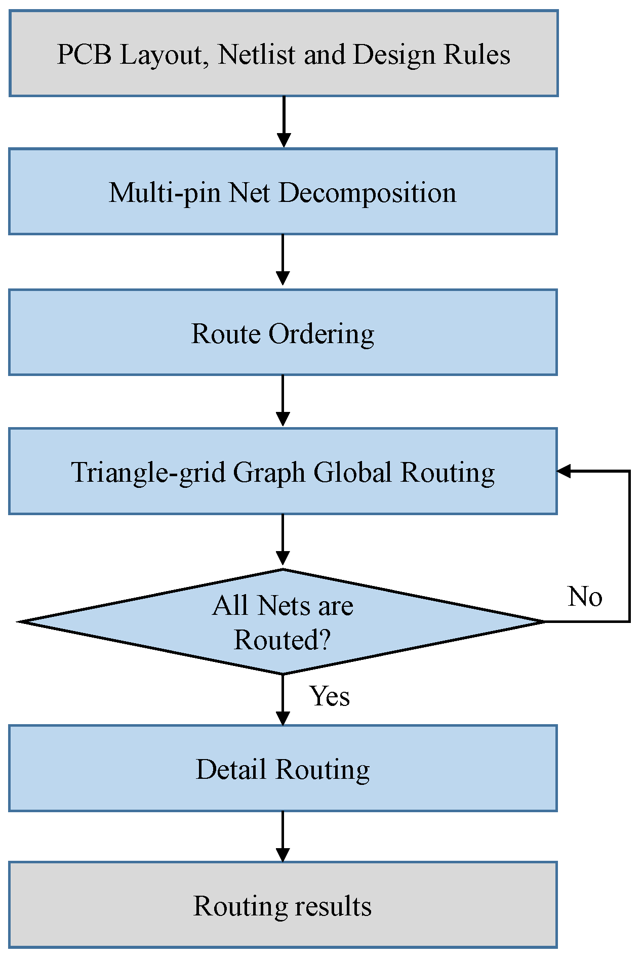
In this section, we present our routing algorithm. Figure 5 summarizes our algorithm flow, which consists of four major stages. The algorithm flow comprises four primary stages. Firstly, we begin by decomposing all multi-pin nets into two-pin nets, utilizing the information obtained from the PCB. This step facilitates the subsequent process of connecting all the nets comprehensively, thus enhancing the overall routability of the design.

Figure 5.
The flow of our algorithm.
Following that, we establish a routing order to determine the sequence in which the nets will be connected. This step is essential for efficient routing. Subsequently, we construct a triangular grid graph and carefully select the starting and ending points that are crucial for the max-flow pathfinding process. This ensures an approximately optimal pathfinding solution.
Lastly, once all the unconnected nets have been planned, we proceed with the detailed routing phase to achieve the final routing result. This stage involves meticulous attention to detail in order to maximize the effectiveness and reliability of the routing process.
3.1. Multi-Pin Nets Decomposition
The shortest path problem for two-pin nets is one of the fundamental challenges in PCB routing. It involves finding the shortest routing path between two pins, taking into account any obstacles present on the PCB. However, in practical routing scenarios, nets often comprise more than just two pins. To address this issue, a common approach is to decompose multi-pin nets into a series of two-pin nets.
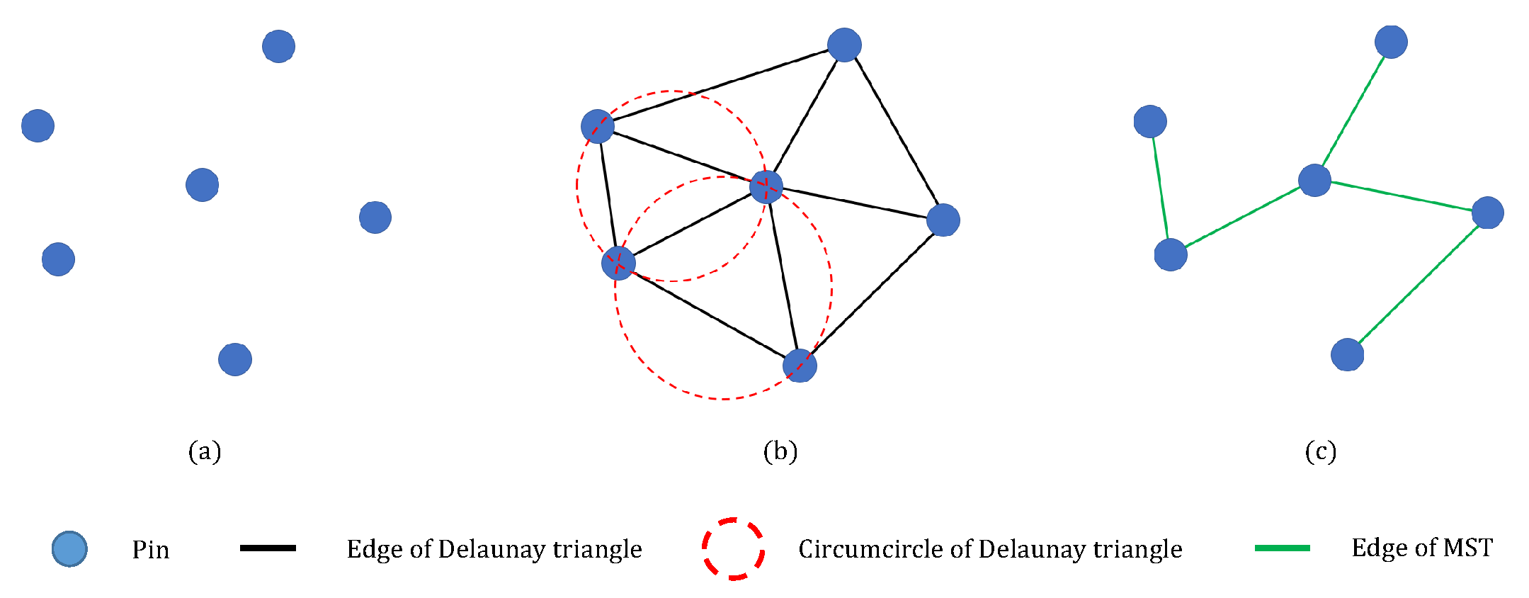
The first step in this decomposition process is to view all the pins within a multi-pin net as individual points and apply the Delaunay triangulation [20]. This method maximizes the sum of the interior angles of all generated triangles while avoiding the creation of highly acute triangles (refer to Figure 6b).
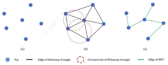
Figure 6.
An example of multi-pin nets decomposition. (a) All the pins in a net. (b) Delaunay triangles composed of pins. (c) A minimum spanning tree constructed by pins.
Next, the Kruskal algorithm is used to construct the minimum spanning tree (MST) for all the points which have a lower complexity compared to the minimal Steiner tree. In this tree, the weight of each edge corresponds to the distance between the two points (refer to Figure 6c).
Finally, any connections that violate the set rules are removed, for example, two connected pins are not allowed to connect within the same component, or one pin should not have more than one connection, resulting in the generation of the required two-pin nets.
The time complexity of the Delaunay triangulation construction is [20], where p is the number of pins. The complexity of constructing the minimum spanning tree is . Therefore, the complexity of multi-pin nets decomposition is .
3.2. Route Ordering
The routing order has an important effect on the quality of the routing, so we propose an algorithm to determine the routing order in this section. Note that the overall connection relationship on a PCB can be quite complex, with potentially numerous connections between each component. To address this issue, we can consider a hypothetical scenario where the PCB predominantly consists of larger components that are connected to smaller ones. Additionally, there exists a definite connection relationship between these larger components, forming a composite star topology. The basic idea behind the Comp-Star algorithm for sequencing involves decomposing the routing graph into smaller components, routing the pin pairs within these smaller components first, connecting the small components to the larger ones, and finally, establishing connections between the larger components themselves.
It is worth noting that this problem can be classified as a vertex cover problem, which is known to be NP-complete. As a result, finding an optimal solution in deterministic polynomial time is challenging. Nonetheless, there are several approximate algorithms available that can identify the minimum value of vertex coverage in a given undirected graph. One such algorithm is the 2-approximation algorithm, which can be utilized to find a vertex cover set that is at most twice the size of the optimal vertex cover. As illustrated in Figure 7, the first step involves constructing the connection graph using the components as vertices. These components can be in the form of pads, vias, or complex footprints. An edge in the graph represents a connection between two components, with at least one net linking them. The weight assigned to each edge corresponds to the number of nets between the two components. To distinguish the importance of each component, a weight function is defined on the vertex set . This weight function assigns higher priority to components with more nets. For a given vertex , the number of nets containing at least one component pin associated with v is denoted as . The weight function is defined as follows.
where the constants . We consider the minimum-weight vertex cover problem on the graph . Our Comp-Star algorithm applies Bar-Yehuda and Even’s algorithm, which constructs both a primal integral solution and a dual feasible solution simultaneously, without solving either the primal or dual programs. This approach is known as the primal-dual schema and provides a 2-approximation for finding the minimum-weight overlapping cover [21]. The time complexity of the algorithm is , where n represents the number of vertices and m represents the number of edges in the graph .
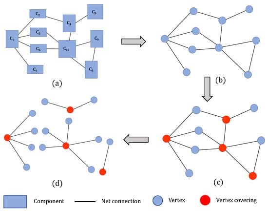
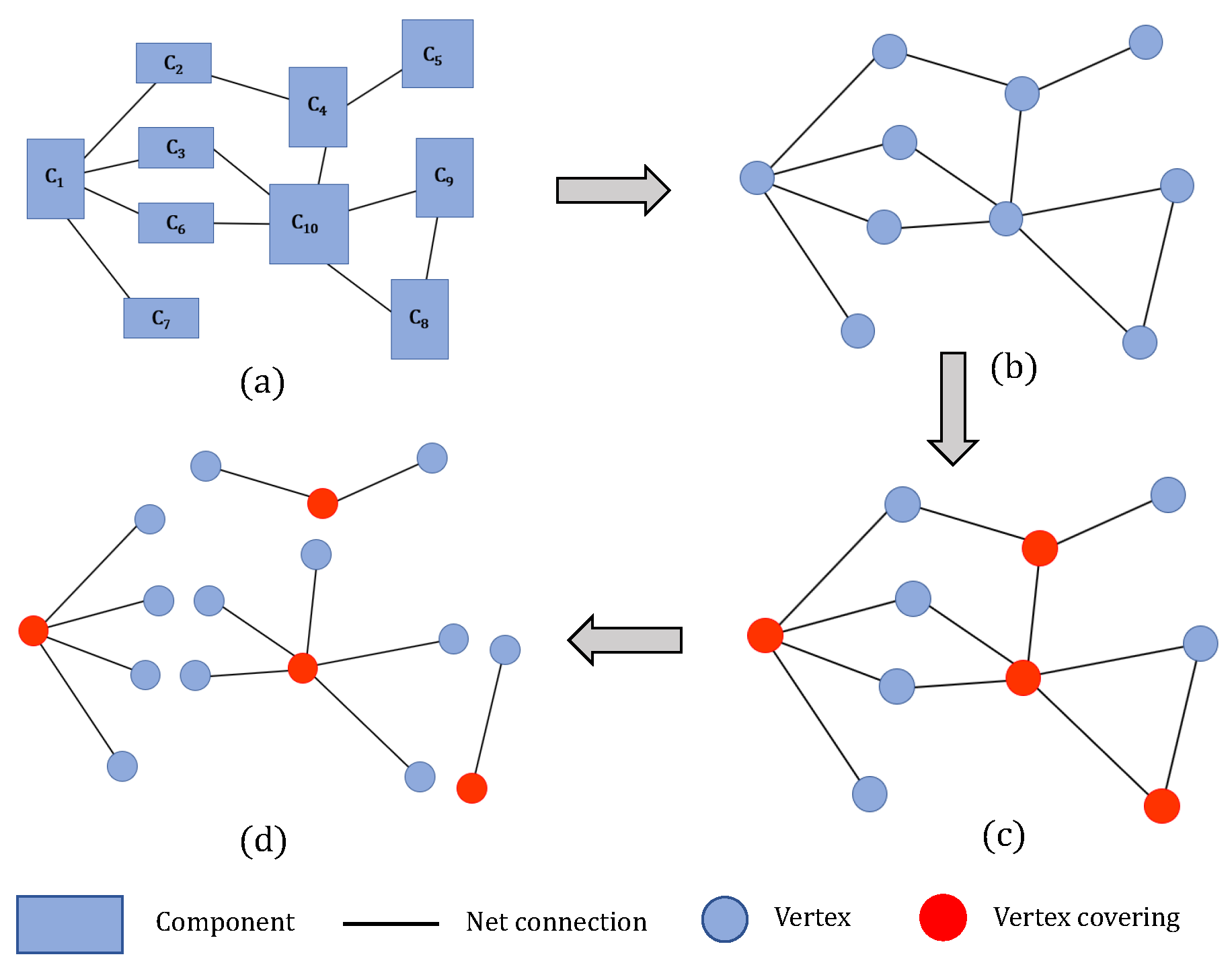
Figure 7.
An example of component graph construction and decomposition. (a) The schematic diagram of a PCB in the current layout. (b) Constructing a component graph by shrinking all the pins in the same component into a vertex and reserving their connections by an edge. (c) Searching for a minimum vertex covering of the graph and coloring them red. (d) Decomposing the component graph into multiple component stars such that the main component is colored red.
Based on the results obtained from Algorithm 1, we are able to identify all the component stars. We select the first component in the queue Q, which is considered the most important, and proceed to route it first. To begin routing, we choose a net that has the shortest distance between two pins within the component. From there, we can either route clockwise or counterclockwise around this net. Once this component has been successfully routed, we move on to the next component in the queue and route its unconnected nets. We continue this process of selecting and routing component stars until the queue Q is empty, thus determining the entire routing order.
| Algorithm 1 Comp-Star decomposition |
|
3.3. Global Routing Based on Triangular Grid
In this section, we present a novel global routing algorithm that forms the core of our methodology. By utilizing a triangular grid graph and a maximum flow model, the algorithm efficiently discovers paths for global planning. The algorithm consists of four main stages. In the initial stage, we construct a global triangular grid graph, enabling us to effectively identify and utilize all available routing resources on the PCB. Moving to the second stage, we update the graph based on the determined routing order. In the third stage, we formulate the global routing problem as a maximum flow model. To solve this model, we employ the Edmonds–Karp algorithm [22], which efficiently discovers the global routing.
3.3.1. Triangular Grid Graph Construction
We consider all items on the printed circuit board as vertices in our diagram, including center points of pads, vias or obstacles, boundary vertices, and end points of tracks. These vertices are treated as obstacles, restricting direct passage. We then calculate the Euclidean distance between all pairs of vertices and sort them. Using an R-tree, we add edges to the graph and determine if they intersect with existing edges. Once all edges are constructed, we start from the first edge and traverse all connected vertices to build the first triangular face, and then we repeat this process to locate all triangular faces. We record all vertex, edge, and face relations as and construct the triangular grid graph , where V represents the set of vertices, E represents the set of edges, and F represents the set of faces, as shown in Figure 8.
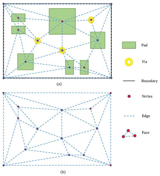
Figure 8.
An example of triangular grid graph construction. (a) The schematic diagram of a case of PCB. (b) Constructing a triangular grid graph.
We choose to use triangles instead of rectangles to reduce model size and simplify construction and calculation. Assuming there is only one pad in each footprint on the printed circuit board and n pads in total, the number of vertices generated in the triangular grid graph is . If we were to use a rectangle grid like the Hanan grid, we would need to include even more vertices—totaling over —as we would need to add the vertices of the boundary of each pad’s component. This would result in a great increase in the number of data needed to represent the graph. Furthermore, traversing each cell in the Hanan grid would take significantly longer than in the triangular grid.
3.3.2. Graph Local Modification
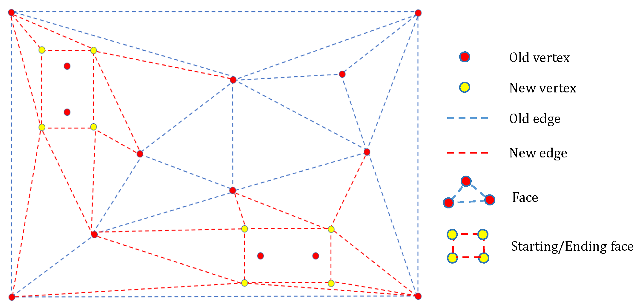
Our model not only supports the sequential routing of nets in a given order but also enables the simultaneous routing of multiple nets with adjacent starting and ending points. This is achieved by merging several nets into a super-net. Prior to routing, we must update the area where the starting and ending points are located. Using the triangular grid graph G as a basis, we delete the vertices, edges, and faces where the starting and ending points reside. Then, we construct the smallest rectangular grid that can contain all starting points as the starting face, and the same is performed for the ending face. These rectangular faces are constructed to ensure that the paths are at a 90-degree angle from the starting or ending points, which facilitates subsequent path search and calculations. The remaining vertices are then reconnected to construct a new dynamic updating graph , as shown in Figure 9.

Figure 9.
An example of triangular grid graph modification.
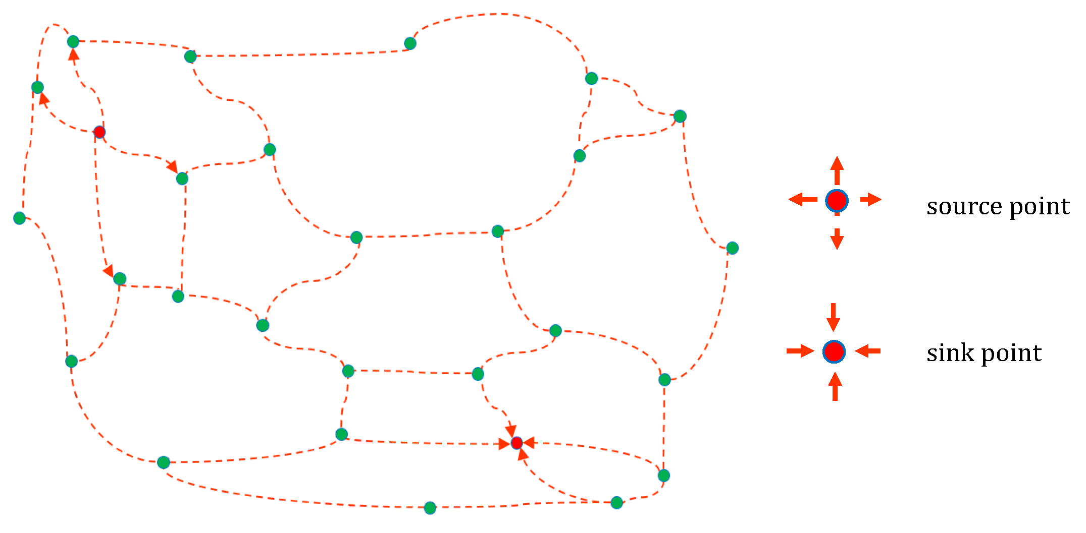
In , we can identify edge sequences that represent the gaps and regions that the routing must traverse. Each face in is viewed as a point, and the dual graph of this graph is a flow network, as depicted in Figure 10. In this network, the starting face serves as the source point and the ending face serves as the sink point. The direction of the network is always from the source point to the sink point, and the capacity of the network is defined as the maximum capacity allowed on each edge in . Therefore, can also be interpreted as a flow network model, where the vertices of correspond to the faces of and the edges of pass through the edges of .
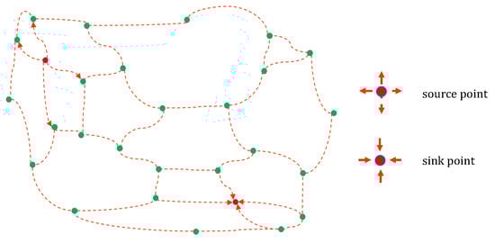
Figure 10.
The dual graph of dynamic updating graph.
3.3.3. Capacity Definition
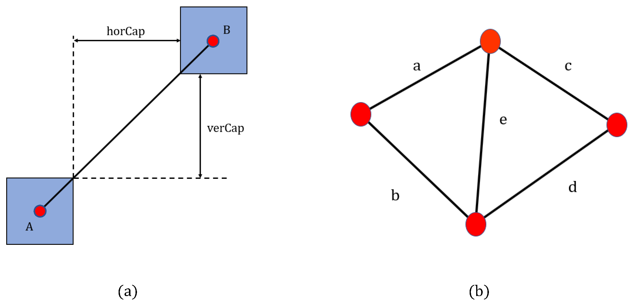
In the graph , the capacity of all edges should be determined based on the actual boundary of the PCB items corresponding to the vertices, rather than simply calculating the Euclidean distance between the two vertices on the edge. Figure 11 illustrates this concept, where the vertices A and B correspond to rectangular items. We define the left-bottom coordinate and right-top coordinate of their boundary as and , respectively. The horizontal capacity, vertical capacity, and maximum capacity of this edge are denoted as , , and , respectively, and they can be calculated as follows:

Figure 11.
The diagram of capacity calculation. (a) An example of an edge with its two vertices. (b) An example of two adjacent triangular grids.
By applying these equations, we can obtain the preliminary capacity of all edges. However, in order to reduce the error, we need to calculate the capacity of edges that do not belong to the starting face and ending face a few more times. This is because there is a relationship among the capacities of each edge in a triangular grid. As shown in Figure 11b, when calculating the capacity of an edge e, we consider the two adjacent triangular grids that share the edge, as well as the other edges a, b, c, and d of these grids. The capacity can be calculated as follows:
By incorporating these iterative calculations, the capacity of the entire graph will reflect the actual boundaries of the PCB items more accurately. Consequently, this refined capacity estimation will yield improved results when searching for the maximum flow.
3.3.4. Global Routing Problem Modeling
We have provided the fundamental definition of the maximum flow model in Section 2.1 and introduced our network flow model in Section 3.3.2. Now, we can integrate the current global routing problem into our constructed model. The notation utilized in this section is summarized in Table 1.

Table 1.
Notation description in global routing problem modeling.
According to the graph , we officially declare the global routing problem to be an integer linear programming (ILP) formulation as follows:
We propose a model for computing the optimal flow of nets in a given graph , where each face of the graph represents a possible area for routing the nets. We define directed flows as those where i and j correspond to the center points of two faces, and is the edge shared by these faces. The decision variable denotes whether net k flows through the edge , and it can only take values of 0 or 1. The objective function (10) aims to minimize the cost of routing nets through the graph, where is the cost of net k on edge , typically defined as the distance between i and j.
To ensure a feasible routing solution, we impose four constraints on the model. Constraints (10a) and (10b) ensure that the maximum flow of each net is limited, and the flow must follow the direction from the source to the sink . The maximum value of n corresponds to the total number of nets, in order to maximize the total flow. Constraint (10c) guarantees balance between the net flows entering and leaving each vertex, except for the source and sink vertices. This is the most fundamental constraint of the network flow model, ensuring that each net path is continuous from start to end. Finally, constraint (10d) limits the total flow of all nets on each edge, considering their capacity and the flow value of each net.
Due to the strict constraints and decision variables of the maximum flow problem, solving this ILP problem is NP-hard, requiring enormous time and computational resources. For a medium-sized PCB, the runtime may require several hours [23]. To address this, we apply maximum flow algorithms to more efficiently solve the problem.
3.3.5. Maximum Flow Algorithm Pathfinding
A maximum flow can only be achieved through available edges from the starting face to the ending face. While obtaining the specific value of this maximum flow is not necessary, it is crucial to find all the augmenting paths of the graph. Our algorithm utilizes the Edmond–Karp (EK) algorithm, which employs the Breadth-First Search (BFS) method to locate these paths.
To begin, we use a minimum priority queue Q to store the visited face and its weight, sorting elements from smallest to largest by their weight. We set the starting face and its initial weight value and add it to Q. We then iterate through the elements in the queue, obtaining the current face and continuing to find adjacent faces, updating their weights, and adding them to the queue.
When the face reaches the ending face, we retrace all the visited faces to obtain the result of the augmenting path. Lastly, we update the flow value of all the edges that the path goes through. Each time we search for a net, we find an augmenting path.
Algorithm 2 provides the pseudo-code for our process.
| Algorithm 2 Our maximum flow algorithm |
|
In Algorithm 2, the includes several conditions:
- Forward arc condition: The sum of the flow value of an edge and the new flow value cannot exceed the edge’s capacity.
- Backward arc condition: The flow value of an edge cannot be less than the new net cost, i.e., the difference between the flow value and the net cost must be greater than or equal to zero.
- Access condition: This face must not have been visited before.
The correctness of the max-flow algorithm can only be guaranteed if these three conditions are satisfied. The first two conditions are significant as they ensure the existence of augmented paths in the flow network, as discussed in Equation (3). The calculation of the weight is as follows.
where represent the center of the next face , the starting point, the ending point, the middle point of all starting points, and the middle point of all ending points, and their coordinates will be added to the calculation. is the formula for calculating the Manhattan distance between two points:
The term refers to a guide line that connects directly from to . This guide line adjusts the weight of the faces it passes through to concentrate all wires in the intermediate region, thereby improving the utilization and routability of the routing area. The constants also play an important role in determining W. When , the algorithm’s result will be closer to the guide line. On the other hand, if is not much larger than and , the algorithm’s result depends more on a heuristic search, which may deviate significantly from the expected outcome and require more time.
The algorithm is called in a loop. Once augmented paths in the form of triangular grids are found for all nets, the flow values on edges of are updated, and the directions of flows passing through all edges roughly follow from the source point to the sink point. The time complexity of the algorithm is , where m is the number of nets and n is the number of faces in the graph .
3.3.6. Flow Decomposition
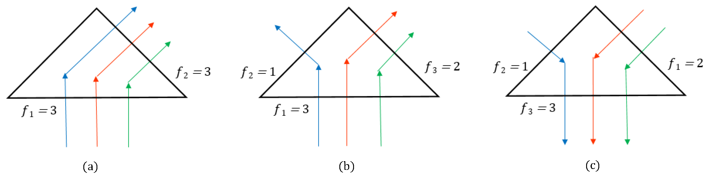
We utilize flow decomposition to extract the approximate set of routing paths for each net. This technique enables us to determine the number and direction of flows that can pass through each edge, based on the flow value and previously obtained face paths. In triangular grids, there are only three simple cases of flow direction on each triangular face, as illustrated in Figure 12.
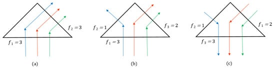
Figure 12.
Three cases of the direction of the flows (a) One edge in and one edge out. (b) One edge in and two edges out. (c) Two edges in and one edge out.
Based on the three aforementioned cases, our triangular grid algorithm has an edge over rectangular ones as it can easily decompose flow. In rectangular grids, the number and direction of flow in each of the four edges make the situations to be discussed more numerous and complicated. To avoid crossing during decomposition, we follow the “same direction principle”. We start by obtaining the first starting point , the first ending point , and the last ending point , and then we obtain a cross product :
In a triangular grid face, we obtain the midpoint of the current edge and the midpoint on the other two edges of the face, and we obtain another cross product :
If the directions of and are the same, the situation indicates that vectors to and to have been rotated clockwise or counterclockwise in the same direction. We choose to use edge for flow decomposition, and if it is not feasible, edge is chosen. We then subtract the flow value of the chosen edge from the total flow value of the wire which includes the wire width and spacing to ensure that the decomposed path satisfies the constraints. If the flow value of one of the edges is 0, we consider choosing the other edge. We ensure that paths starting from other starting points are as similar as possible to paths that have been in decomposition in turn and there is no crossover. Finally, we obtain the planned paths of all wires, which can be used in future detail routing. These paths are added to the triangular grid graph and partake in the global routing of the rest of the unrouted nets.
3.4. Detail Routing
After the global routing process, the planned path is determined for each unconnected net. To convert these paths into complete wires, various factors need to be taken into account during the detail routing stage. These factors include wire width, spacing, real obstacle boundaries, and achieving a well-structured topology, all while adhering to the rules of routing design.
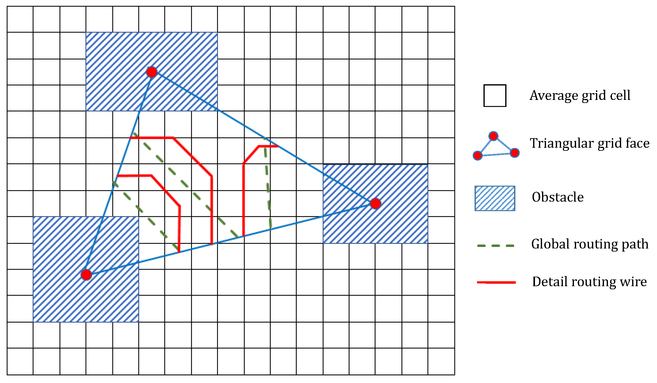
To achieve this, we propose the construction of an average grid that spans the entire printed circuit board. Each cell in this grid represents the smallest allowable square width on the board. As depicted in Figure 13, when the planned paths are obtained within a triangular grid face, we can project each path onto the average grid. Subsequently, a series of lines are drawn parallel, perpendicular, or intersecting with the grid lines at a angle based on these paths. These lines are then connected sequentially, resulting in a specific wire corresponding to that particular path.
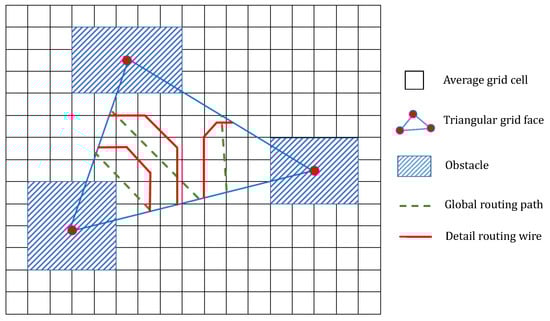
Figure 13.
A schematic diagram of detail routing.
We repeat this adjustment process for the remaining paths, considering the position and direction of the first wire as well as the aforementioned factors, such as calculating the spacing from the first wire and the wire width of the current wire, until all specific wires are calculated and routed accordingly.
4. Experimental Results
We implemented our algorithm using the C++ programming language and conducted all experiments on a single machine equipped with an Intel Core 3.40GHz CPU and 16 GB of memory. Table 2 presents the benchmarks for the industry-designed PCBs, where the dimensions of width and height are denoted by “”. “”, “”, “”, and “” denote the numbers of PCB pads, vias, routed tracks, and unrouted nets, respectively.
Table 2.
Benchmark PCB design statistics.
4.1. Effectiveness of Route Ordering
To evaluate the effectiveness of our proposed route ordering algorithm, we conducted additional experiments comparing the results with and without the ordering method. A summary of the routing results, including routability, runtime, and the total number of design rule violations (DRVs), is presented in Table 3.
Table 3.
Comparison of routing results without ordering and with ordering.
In scenarios where no ordering was applied, there was a significant amount of randomness in the selection of nets to be routed. As a consequence, the starting and ending points of these nets could be widely dispersed, making it impractical to utilize our updated triangular grid graph to combine them as a cohesive flow for global path searching. This resulted in considerable time overhead.
Moreover, due to the poor results from the global routing stage, the specific wires after the detailed routing process could occupy excessive space that could have been utilized by other nets. Furthermore, there were no methods available to mitigate the number of conflicts in the routing space, such as using techniques like rip-up and reroute. Consequently, this led to a decrease in routability and an increase in the number of DRVs.
4.2. Comparison with State-of-the-Art Routers
We compared our algorithm with two state-of-the-art non-academic routers, FreeRouting [24] and Cadance Allegro [25]. FreeRouting is an open-source PCB routing software written in Java that is widely used. Cadence Allegro is a leading commercial tool for PCB design, which is a high-end software in Electronic Design Automation (EDA) tools. We used the default setting for both routers and applied the same input designs and design rules in our experiments. We selected examples where the components were separated from each other to facilitate bus routing, and our algorithm was implemented on other commercial software to clearly demonstrate the routing results.
Table 4 summarizes the experimental results by comparing the routability, runtime, and design rule violations (DRVs) of the three routers. A hyphen in the table indicates that the design could not run on the software or that the running time exceeded one hour. As shown in the table, our algorithm outperforms FreeRouting and Allegro in terms of routability, runtime, and DRVs. It should be noted that these two routers use a serial approach to routing, meaning that only one net is selected at a time for routing. They do not use global planning before routing, which causes them to reassess congestion on the board after every wire has been routed. If enough space is not available for routing, they take measures such as layer reassignment, rip-up, and reroute, resulting in additional time and space costs. However, our algorithm tries to route all the nets on the same layer, resulting in better results.
Table 4.
Comparison of routing results between FreeRouting, Allegro, and ours.
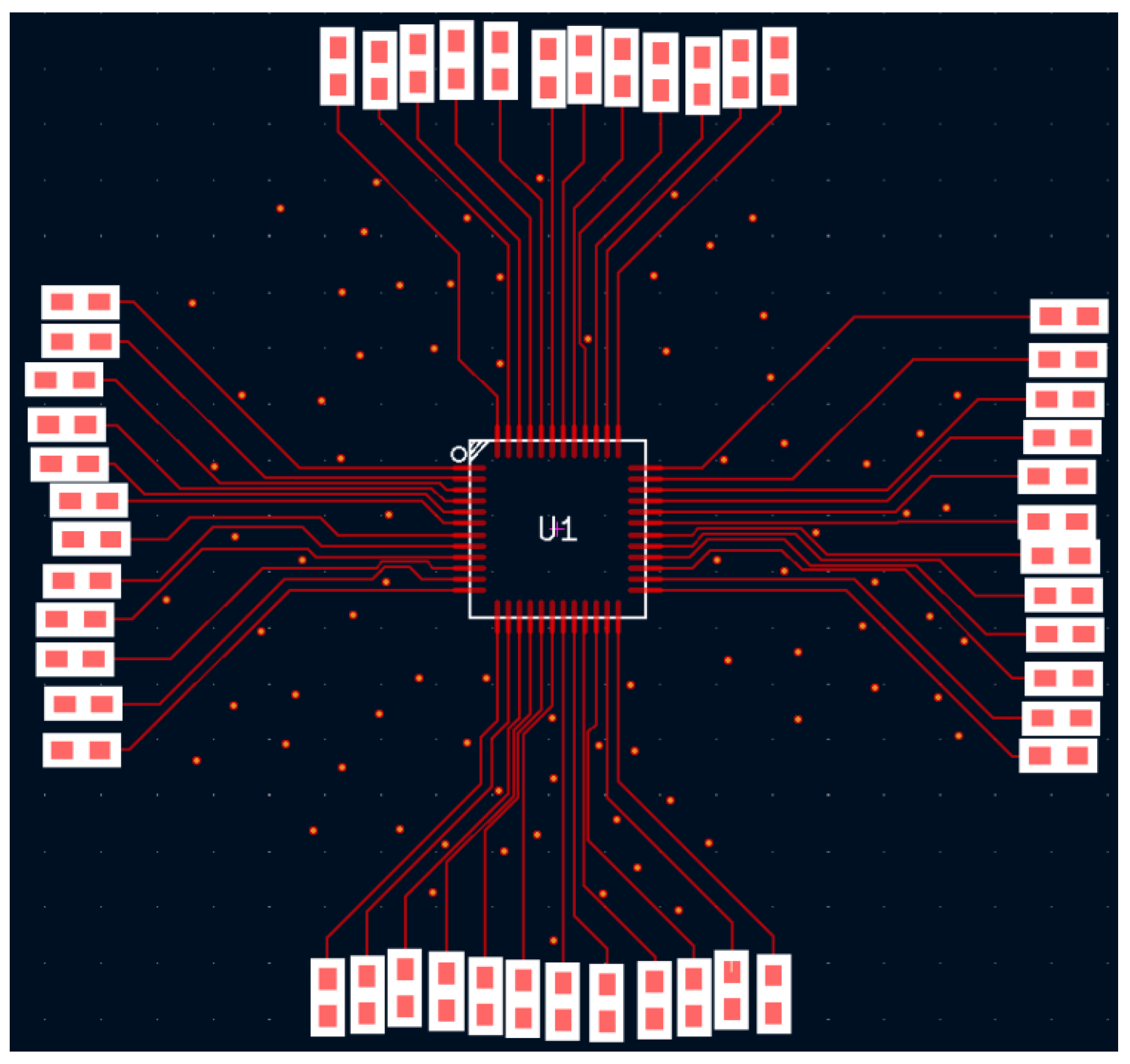
Figure 14 shows the routing result of PCB5 using our algorithm. After the Comp-Star decomposition algorithm runs, the component is selected as the component star, and the net of the seventh pad counted from the top down on its left side has the shortest length, making it the first net to be routed. All 12 nets to the left of have adjacent starting and ending points, so they can be routed simultaneously in the global triangular grid, with all completed wires concentrated in the center region. Finally, the remaining nets are routed according to the clockwise routing sequence, taking into account pads, vias, and tracks on the board as obstacles. These results demonstrate that our algorithm is effective, applicable, and efficient in routing PCB designs.
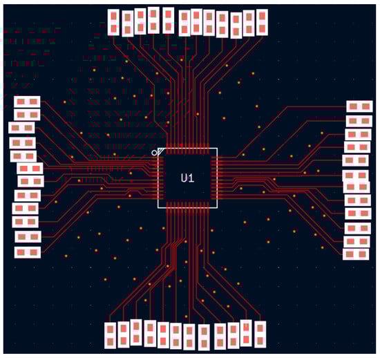
Figure 14.
The result of PCB5.
5. Conclusions
In this paper, we have presented a novel global routing algorithm for PCB designs that takes into account the 135-degree routing requirements. Additionally, we have incorporated the use of the Comp-Star decomposition algorithm to determine the routing order for the nets. This algorithm helps identify the most critical components that should be given priority during the routing process, thereby reducing congestion and wire crossover. We have proposed a triangular grid model that enables more effective searching for optimal paths during the global routing stage. Furthermore, by employing the maximum flow scheme, we can efficiently find paths that connect all the nets, ensuring a complete global routing stage. Extensive experimental comparisons with two state-of-the-art routers demonstrate the superiority of our algorithm in terms of performance.
Author Contributions
Conceptualization, J.C. and Q.L.; methodology, J.C., Y.Z. and Q.L.; software, Y.Z. and X.Z.; validation, J.C. and Y.Z.; formal analysis, J.C., Y.Z. and Q.L.; writing—original draft preparation, J.C. and Y.Z.; writing—review and editing, J.C., Y.Z. and Q.L.; funding acquisition, J.C. All authors have read and agreed to the published version of the manuscript.
Funding
This research was funded by NSFC grant number 61977017.
Data Availability Statement
The data are unavailable due to privacy restrictions.
Acknowledgments
The authors want to thank the editor and anonymous reviewers for their 330 valuable suggestions for improving this paper.
Conflicts of Interest
The authors declare no conflict of interest.
References
- Hu, J.; Sapatnekar, S.S. A survey on multi-net global routing for integrated circuits. Integr. VLSI J. 2001, 31, 1–49. [Google Scholar] [CrossRef]
- Xu, Y.; Zhang, Y.; Chu, C. FastRoute 4.0: Global router with efficient via minimization. In Proceedings of the Asia and South Pacific Design Automation Conference Proceedings, Yokohama, Japan, 19–22 January 2009; pp. 576–581. [Google Scholar]
- Chang, Y.J.; Lee, Y.T.; Wang, T.C. NTHU-Route 2.0: A fast and stable global router. In Proceedings of the IEEE/ACM International Conference on Computer-Aided Design, San Jose, CA, USA, 10–13 November 2008; pp. 338–343. [Google Scholar]
- Cho, M.; Pan, D.Z. BoxRouter: A new global router based on box expansion and progressive ILP. IEEE Trans. Comput.-Aided Des. Integr. Circuits Syst. 2007, 26, 2130–2143. [Google Scholar]
- Qi, Z.; Cai, Y.; Zhou, Q.; Li, Z.; Chen, M. VFGR: A very fast parallel global router with accurate congestion modeling. In Proceedings of the Asia and South Pacific Design Automation Conference Proceedings, Singapore, 20–23 January 2014; pp. 525–530. [Google Scholar]
- He, J.; Burtscher, M.; Manohar, R.; Pingali, K. SPRoute: A scalable parallel negotiation-based global router. In Proceedings of the IEEE/ACM International Conference on Computer-Aided Design, Westminster, CO, USA, 4–7 November 2019; pp. 1–8. [Google Scholar]
- Liu, J.; Pui, C.-W.; Wang, F.; Young, E.F. CUGR: Detailed-routability-driven 3d global routing with probabilistic resource model. In Proceedings of the ACM/IEEE Design Automation Conference, Virtual, 20–24 July 2020; pp. 1–6. [Google Scholar]
- Jiang, Y.-J.; Fang, S.-Y. COALA: Concurrently assigning wire segments to layers for 2D global routing. In Proceedings of the IEEE/ACM International Conference on Computer-Aided Design, San Diego, CA, USA, 2–5 November 2020; pp. 1–8. [Google Scholar]
- Kong, H.; Yan, T.; Wong, M.D.F. Automatic Bus Planner for Dense PCBs. In Proceedings of the ACM/IEEE Design Automation Conference, San Francisco, CA, USA, 26–31 July 2009; pp. 326–331. [Google Scholar]
- Lin, S.-T.; Wang, H.-H.; Kuo, C.-Y.; Chen, Y.; Li, Y.-L. A Complete PCB Routing Methodology with Concurrent Hierarchical Routing. In Proceedings of the Design Automation Conference DAC, San Francisco, CA, USA, 5–9 December 2021; pp. 1141–1146. [Google Scholar]
- Yan, J.-T.; Chen, Z.-W. Obstacle-aware length-matching bus routing. In Proceedings of the International Symposium on Physical Design, Santa Barbara, CA, USA, 27–30 March 2011; pp. 61–68. [Google Scholar]
- Ozdal, M.M.; Wong, M.D.F. A length-matching routing algorithm for high-performance printed circuit boards. Electr. Comput. Eng. 2006, 25, 2784–2793. [Google Scholar]
- Ozdal, M.M.; Hentschke, R.F. Exact route matching algorithms for analog and mixed signal integrated circuits. In Proceedings of the ACM/IEEE Design Automation Conference, San Francisco, CA, USA, 26–31 July 2009; pp. 231–238. [Google Scholar]
- Kim, D.; Do, S.; Lee, S.-Y.; Kang, S. Compact Topology-Aware Bus Routing for Design Regularity. IEEE Trans. Comput.-Aided Des. Integr. Circuits Syst. 2020, 39, 1744–1749. [Google Scholar] [CrossRef]
- Chen, J.; Liu, J.; Chen, G.; Zheng, D.; Young, E.F.Y. MARCH: MAze routing under a concurrent and hierarchical scheme for buses. In Proceedings of the ACM/IEEE Design Automation Conference, Las Vegas, NV, USA, 2–6 June 2019; pp. 1–6. [Google Scholar]
- Hsu, C.-H.; Hung, S.-C.; Chen, H.; Sun, F.-K.; Chang, Y.-W. A DAG-Based Algorithm for Obstacle-Aware Topology-Matching On-Track Bus Routing. IEEE Trans. Comput.-Aided Des. Integr. Circuits Syst. 2021, 40, 533–546. [Google Scholar] [CrossRef]
- Zhang, H.-T.; Fujita, M.; Cheng, C.-K.; Jiang, J.-H. SAT-Based On-Track Bus Routing. IEEE Trans. Comput.-Aided Des. Integr. Circuits Syst. 2021, 40, 735–747. [Google Scholar] [CrossRef]
- Lin, T.-C.; Merrill, D.; Wu, Y.-Y.; Holtz, C.; Cheng, C.-K. A Unified Printed Circuit Board Routing Algorithm with Complicated Constraints and Differential Pairs. In Proceedings of the Asia and South Pacific Design Automation Conference Proceedings, Tokyo, Japan, 18–21 January 2021; pp. 170–175. [Google Scholar]
- Bulut, M.; Ozcan, E. Optimization of electricity transmission by Ford–Fulkerson algorithm. Sustain. Energy Grids Netw. 2021, 28, 100544. [Google Scholar] [CrossRef]
- Ito, Y. Delaunay Triangulation. In Encyclopedia of Applied and Computational Mathematics; Engquist, B., Ed.; Springer: Berlin/Heidelberg, Germany, 2015; pp. 332–334. [Google Scholar]
- Bar-Yehuda, R.; Even, S. A linear-time approximation algorithm for the weighted vertex cover problem. J. Algorithms 1981, 2, 198–203. [Google Scholar] [CrossRef]
- Lammich, P.; Sefidgar, S.R. Formalizing the Edmonds-Karp Algorithm. In Interactive Theorem Proving; Blanchette, J.C., Merz, S., Eds.; Springer International Publishing: Berlin/Heidelberg, Germany, 2016; pp. 219–234. [Google Scholar]
- Wu, P.-C.; Ma, Q.; Wong, M.D.F. An ILP-based automatic bus planner for dense PCBs. In Proceedings of the 2013 18th Asia and South Pacific Design Automation Conference (ASP-DAC), Yokohama, Japan, 22–25 January 2013; pp. 181–186. [Google Scholar]
- FreeRouting. Available online: https://freerouting.org/ (accessed on 10 May 2023).
- Candance Allegro. Available online: https://www.cadence.com/ (accessed on 10 May 2023).

Disclaimer/Publisher’s Note: The statements, opinions and data contained in all publications are solely those of the individual author(s) and contributor(s) and not of MDPI and/or the editor(s). MDPI and/or the editor(s) disclaim responsibility for any injury to people or property resulting from any ideas, methods, instructions or products referred to in the content. |
© 2023 by the authors. Licensee MDPI, Basel, Switzerland. This article is an open access article distributed under the terms and conditions of the Creative Commons Attribution (CC BY) license (https://creativecommons.org/licenses/by/4.0/).