Abstract
Advances in deep learning have led to the development of various animal species detection models suited for different environments. Building on this, our research introduces a detection model that efficiently handles both batch and real-time processing. It achieves this by integrating a motion-based frame selection algorithm and a two-stage pipelining–dataflow hybrid parallel processing approach. These modifications significantly reduced the processing delay and power consumption of the proposed MCFP-YOLO detector, particularly on embedded systems with limited resources, without trading off the accuracy of our animal species detection system. For field applications, the proposed MCFP-YOLO model was deployed and tested on two embedded devices: the RP4B and the Jetson Nano. While the Jetson Nano provided faster processing, the RP4B was selected due to its lower power consumption and a balanced cost–performance ratio, making it particularly suitable for extended use in remote areas.
1. Introduction
For the safety of wildlife and humans, it is crucial that mitigation systems for wildlife–vehicle collisions (WVCs) and wildlife–human conflicts (WHCs) detect wildlife in real time. Therefore, the delay between when the wildlife first appears in the image and its detection should be enhanced, particularly on low-power machines with limited computational capabilities, such as embedded systems. These systems, while advantageous for their portability and suitability in remote or challenging environments, pose significant constraints in terms of processing speed and power consumption. Therefore, our work addresses the following critical requirements:
- Fast Processing Speed: The system must process input data and render decisions rapidly to ensure real-time detection. This is vital to effectively mitigate WVCs and WHCs.
- Low Power Consumption: Given the remote locations of wildlife encounters, and the impracticality of frequent battery replacements or high-power solutions, the system must operate with minimal power consumption. This necessitates innovative approaches to model efficiency that do not strain the limited power resources of embedded devices.
- Efficient Deployment on Embedded Systems: Beyond speed and power considerations, the system must be tailored to the unique characteristics of embedded devices, which often have less processing power and memory compared to standard computing systems. This requires a careful balance between model complexity and detection efficacy, ensuring the model is lightweight yet effective.
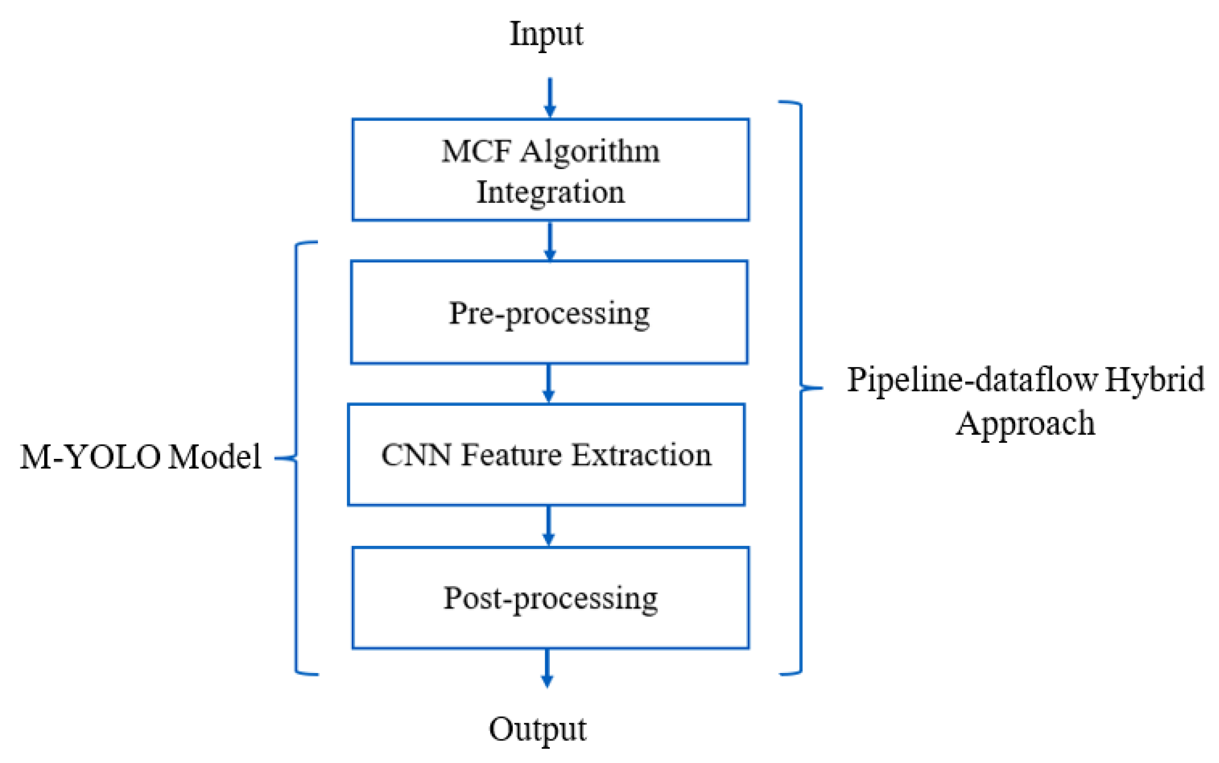
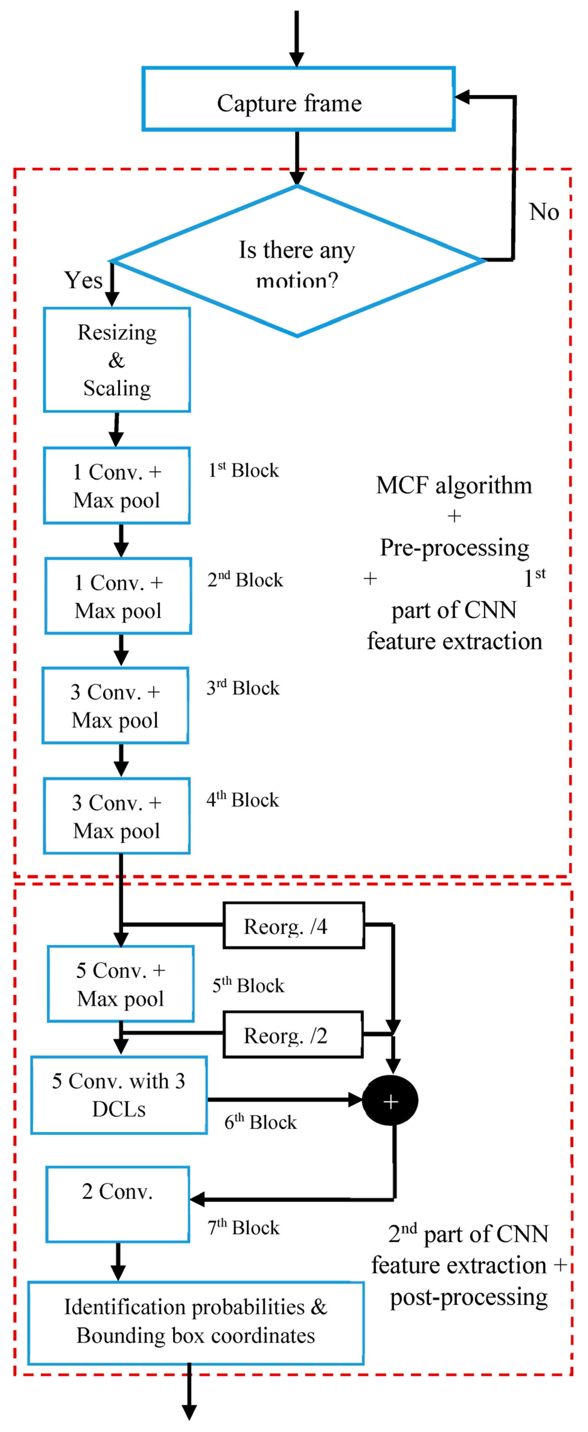
While most researchers propose lightweight object detectors or hardware acceleration techniques to reduce the detection delay and maximize throughput, our work takes a different approach. As shown in Figure 1, we propose the new MCFP-YOLO model, which integrates two ideas into the modified YOLO (M-YOLO) model [1], based on YOLOv2, detailed further in Section 3. These integrations are designed to enhance processing speed and reduce power consumption while maintaining detection accuracy, as the core architecture of the MCFP-YOLO model has not been modified from the original M-YOLO model. The MCFP-YOLO model is designed specifically for deployment in embedded systems. Our contributions can be summarized as follows:
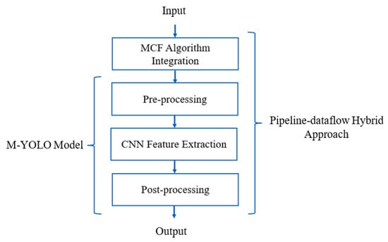
Figure 1.
Workflow diagram illustrating the development of the proposed MCFP-YOLO model from the M-YOLO model by integrating the MCF algorithm and employing parallel processing with the proposed pipeline-dataflow hybrid approach for efficient real-time detection in low-power embedded devices.
- Introduce the Motion-Selective Control Frames (MCF) algorithm to control the number of frames to be processed based on the motion activity within them, which enhances the processing speed and reduces the power consumption of the object detection system.
- Apply a multicore parallel processing technique, which directly minimizes the processing delay of the M-YOLO model, which consists of three sequential tasks [1]: pre-processing, CNN feature extraction, and post-processing, as shown in Figure 1.
- Propose an algorithm that allocates and distributes object detection model layers across pipeline stages to enhance pipelining and improve throughput.
- Propose a novel hybrid approach, integrating pipelining and dataflow, aiming to leverage the throughput advantages of pipelining while integrating the data-driven execution characteristic of dataflow paradigms, especially for conditional processing based on the MCF algorithm.
- Propose the MCFP-YOLO detection model by integrating both the MCF algorithm and parallel processing using the proposed pipeline-dataflow hybrid approach into the M-YOLO model, as shown in Figure 1. The MCFP-YOLO model is designed for embedded devices and is intended to be employed in live camera-based WVC and WHC mitigation systems.
The rest of this paper is organized as follows: Section 2 summarizes related work in enhancing the processing speed of object detection models. Section 3 presents an overview of the M-YOLO model. Section 4 introduces the MCF algorithm. Section 5 describes the parallel processing techniques. Section 6 offers a comparative analysis of the processing speed and power consumption between the proposed MCFP-YOLO detector and the original M-YOLO model. Section 7 evaluates the efficiency of the proposed MCFP-YOLO model on both Raspberry pi 4 model B (RP4B) and NVIDIA Jetson Nano devices. Finally, Section 8 concludes the paper.
2. Related Work
Deploying deep learning-based animal detection models on embedded devices and reducing the processing delay, which is crucial for real-time applications, poses challenges due to their power constraints. Wang et al. [2] offer insights into the development of lightweight models for avian species. This study addresses the balance between model performance and computational efficiency, a key consideration in power-constrained environments. Adami et al. [3] evaluated the performance of YOLOv3 and its lighter version, YOLOv3-tiny, on edge computing devices for detecting deer and wild boar, achieving 82.5% mean Average Precision (mAP) with YOLOv3 and 62.4% mAP with YOLOv3-tiny. Similarly, Sato et al. [4] implemented an animal detection system using YOLOv4 and YOLOv4-tiny to prevent accidents involving animals on highways, reporting accuracies of 84.87% and 79.87%, respectively, with corresponding detection times of 0.035 ms and 0.025 ms. Like our work, the authors deployed their proposed detection system on an embedded device, as proof of the capability of the system.
Additionally, techniques like pruning and quantization have been employed to compress the CNN models and reduce computational workload [5,6], making them suitable for deployment on embedded devices. Although these techniques improve the throughput and reduce the detection delay, they negatively impact the detection accuracy [7,8]. These studies align with our objective of reducing the detection delay. However, instead of refining neural network architectures as carried out in other studies, we examine the neural network inference system from a system’s perspective, targeting the elimination of processing delays. Our aim in this paper is to enhance the processing speed for a given neural network architecture without redesigning the architecture itself.
Other studies have explored the use of Field-Programmable Gate Arrays (FPGAs) for hardware acceleration [9,10]. However, programming them can be complex as it requires knowledge and expertise in hardware programming and optimization. In addition, FPGAs are known for their high power consumption, making power management a critical consideration during their deployment.
Minakova et al. [11] proposed the concurrent use of task-level and data-level parallelism to run CNN inference on embedded devices. This approach ensures high-throughput execution of CNN inference, allowing for optimal utilization of the NVIDIA Jetson, which achieves 20% higher throughput compared to standalone CNN inference.
3. M-YOLO Model
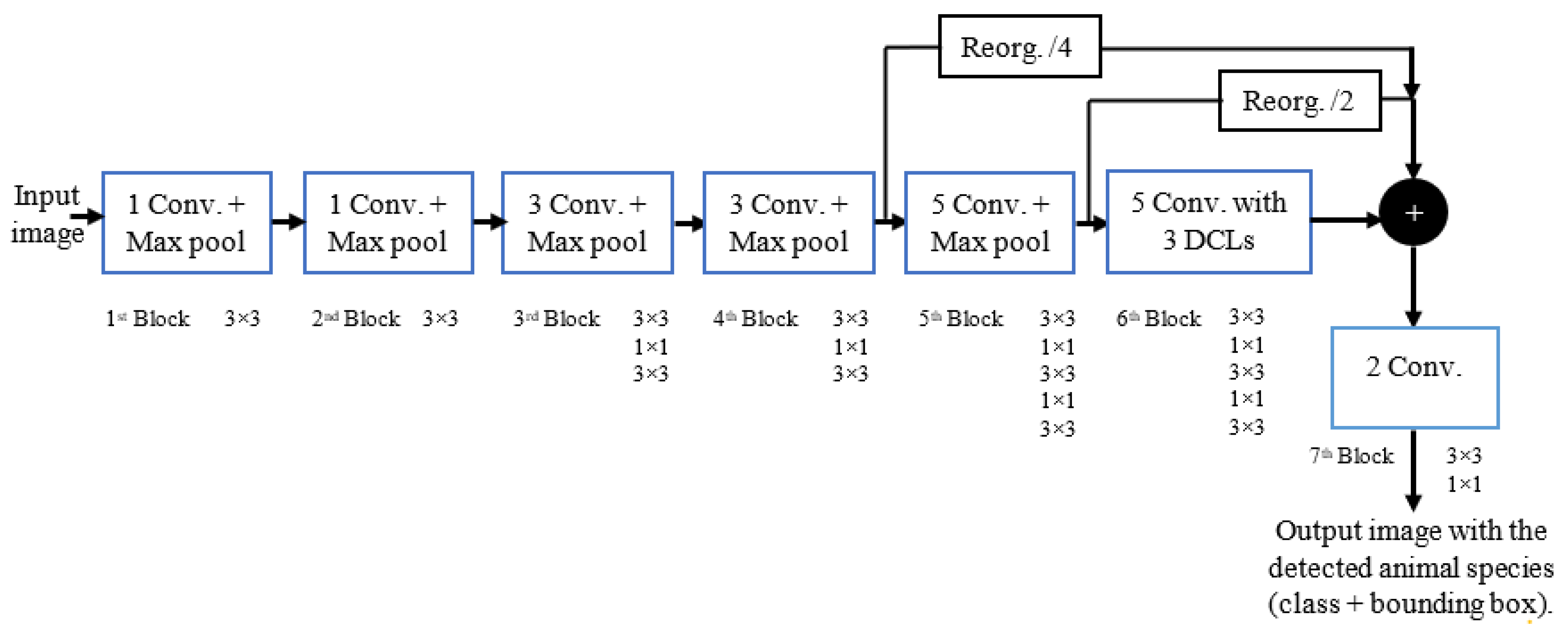
The M-YOLO model [1], a novel detection model based on YOLOv2, was developed specifically for deployment on embedded devices to be used in wildlife mitigation systems, as shown in Figure 2. Compared to the original YOLOv2 architecture, this model underwent three modifications:
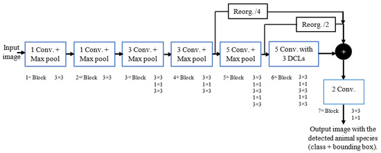
Figure 2.
Architecture of the proposed M-YOLO animal species detector. The detector has a new pass-through layer with a down-sampling factor of 4 to merge low- with high-level features. The sixth block of the detector (blue dashed block) has five convolution layers with three added DCLs [1].
- i.
- Enhancement of extracted features: The proposed M-YOLO model addresses the geometric variations and part deformations of animals by integrating three deformable convolutional layers (DCLs) [1,12]. This allows the model to capture more accurate representations of distinct animal features.
- ii.
- Improvement in species differentiation: The model’s capability to identify six animal species with small differences is improved by incorporating low-level features for multi-level feature merging. This approach enhances the model’s ability to distinguish between closely related species.
- iii.
- Complexity reduction and process acceleration: The complexity of the proposed M-YOLO model is reduced, and the detection process is accelerated without sacrificing the accuracy. This is achieved by removing two repeated 3 × 3 convolutional layers, each with 1024 filters, from the seventh block of the model’s architecture.
The decision to use YOLOv2 as the base model for M-YOLO is driven by its suitability for deployment on embedded devices, particularly in wildlife mitigation systems. YOLOv2 offers an effective balance between processing speed/computational efficiency and accuracy.
While newer versions of YOLO, such as YOLOv5, YOLOv6, etc. offer improvements in various aspects, YOLOv2 provides several advantages for our specific application:
- Computational Efficiency: YOLOv2 is less computationally intensive compared to its later versions. This is a significant factor considering the limited computational capabilities of embedded devices used in our target deployment scenarios.
- Balance Between Speed and Accuracy: YOLOv2 offers a good balance between detection speed and accuracy. For real-time applications in wildlife detection, this balance is crucial as it ensures timely and reliable detection without overwhelming the hardware.
- Customization Ability for Specific Needs: Our modifications to the YOLOv2 architecture, including the integration of deformable convolutional layers, are tailored to address specific challenges in wildlife detection, such as varying animal shapes and sizes. These customizations leverage YOLOv2’s architecture effectively, enhancing its capability to differentiate between animal species and adapt to geometric variations in their appearance.
4. MCF Algorithm
In real-time processing, especially when the detection model is deployed on an embedded device with limited computational capabilities, it is essential to focus computational resources only on frames that have motion. Continuously processing every captured frame can be both resource intensive and power draining. To address this challenge, the MCF algorithm is introduced. By integrating this algorithm into the M-YOLO model, the efficiency will be enhanced in terms of both processing speed and power consumption.
MCF is a pixel-based algorithm that relied on the absolute subtraction technique which compares the pixel values or intensities between two input frames from a live camera or video sequence. The frame differences will decide if there is any moved object in the frame or not. After trial-and-error processing, four consecutive frames from the input are considered at a time and the first frame of each is assumed as a reference frame F(x, y). This strategy of selecting four consecutive frames can be changed depending on the specific requirements of the application, laying the foundation for further enhancement. Equation (1) represents the absolute subtraction of pixel values ∆i(x, y) on the frame Fi (x, y) with the reference frame F(x, y) where i varies from 2 to 4.
where ∆i(x, y) determine if the frame Fi (x, y) has unique information compared to the reference frame F(x, y). If ∆i(x, y) differ from zero, this is an indication of moving objects, while when ∆i(x, y) is equal to zero, this is an indication of stationary objects. However, in reality, it is impossible that ∆i (x, y) will be equal to zero due to the presence of noise. In order to decide if these obtained non-zero values are caused by noise or motion, ∆i (x, y) is compared with a predefined threshold (Th), as shown in Equation (2).
∆i(x, y) = |F(x, y) − Fi (x, y)|
The selection of the threshold value is important. A low threshold value can result in false motion detection because of the presence of noise, where the noisy pixels can be detected as motion pixels, as shown in Figure 3a. The high threshold value can lead to missing motion detection as the small changes in movement will be ignored, as shown in Figure 3c. In our work, the significant value of the threshold is 55 after much trial-and-error processing, as shown in Figure 3b.
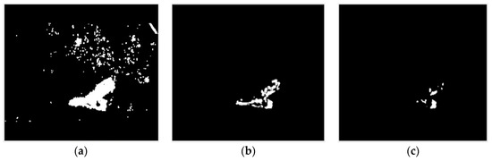
Figure 3.
The visualization comparison after applying different values of threshold: (a) at low threshold = 5, (b) at threshold = 55, and (c) at high threshold = 100.
By taking advantage of this simple technique, only frames that have unique information or animal motion are processed by the M-YOLO detector, leading to a decrease in processing time and power consumption.
4.1. Absolute Subtraction Technique Challenges
There are some challenges that can affect the pixel values [13] and negatively impact the identification of any changes in the frame as motion within a real system. Most of these challenges come from the environmental conditions within the scene, as mentioned in [14], with fewer attributed to the used camera such as:
- Frame noise produced during the acquisition [15].
- Illumination or light intensity variation of the frame’s background.
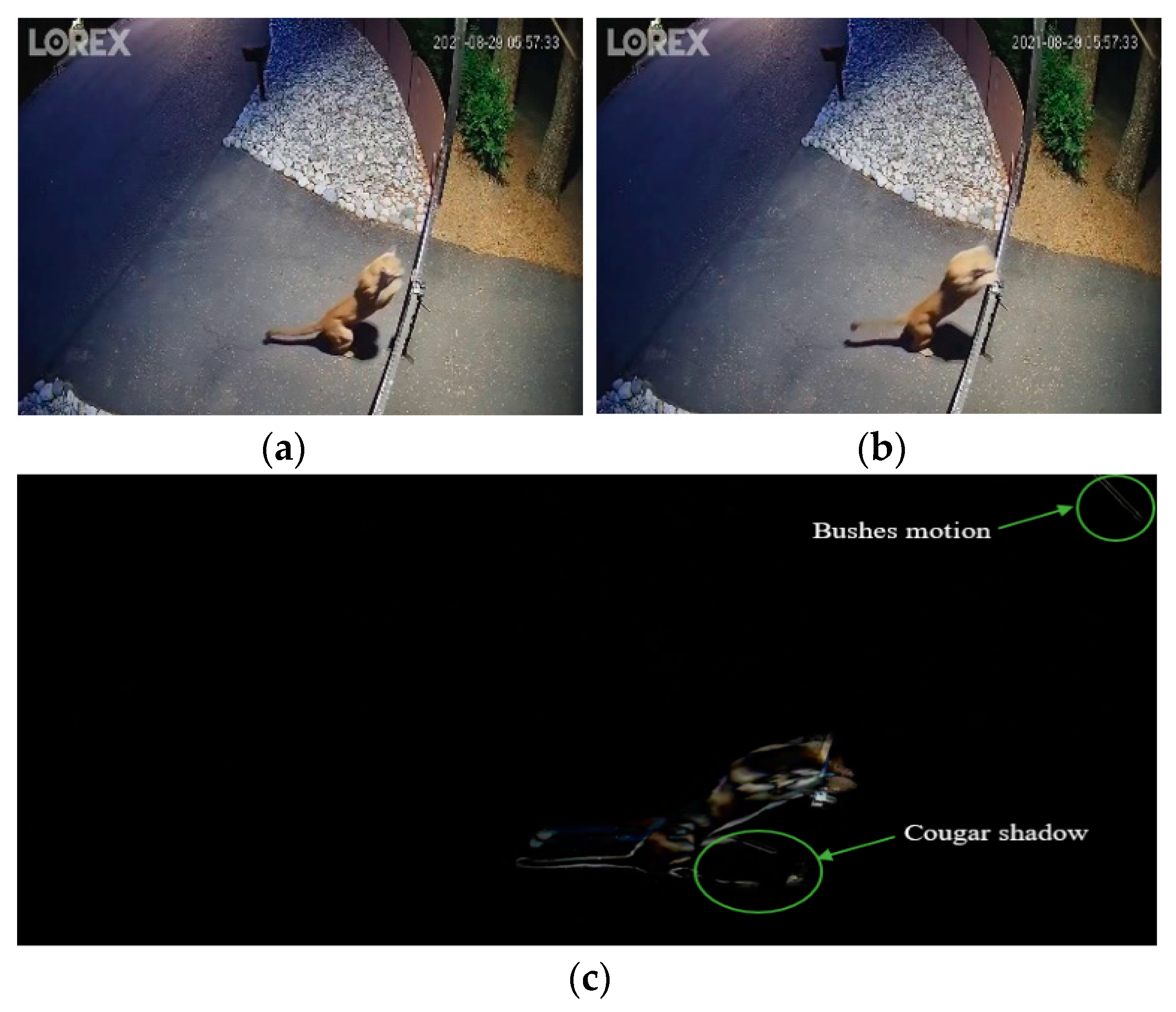
- Dynamic movement of static objects in the background like wind blowing on bushes and trees, as shown in Figure 4c, obtained by applying the absolute subtraction technique between the first frame in Figure 4a and the third frame in Figure 4b.
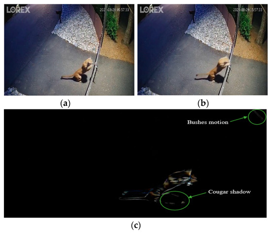 Figure 4. The absolute subtraction technique between (a) the first frame “reference frame”, and (b) the third frame of the four consecutive frames. (c) The resulting output of the absolute subtraction between the two frames with bushes motion and cougar shadow.
 - Shadows of moving objects that can be detected as another moving object, as shown in Figure 4c.
4.2. Improvements to the Absolute Subtraction Technique
To overcome the effects of the above factors, the absolute subtraction technique can be improved by adding a morphological opening operation, which consists of an erosion operation followed by a dilation operation [16]. The erosion operation shrinks the area of detected objects or removes pixels from the object boundaries, otherwise, the dilation operation expands the area of detected objects or adds pixels to the object boundaries [17]. Therefore, the main objective of applying the opening operation is to smoothen contours, remove any isolated bright pixels, and break slight connections between objects in the output image of the absolute subtraction technique. This process helps maintain the shape and size of large objects, as each pixel in the image is adjusted based on the value of its neighboring pixels.
After applying the opening operation, the effect of noise is decreased; however, there is still noise in the frame that is always detected as a motion. A Gaussian filter [18] has been widely used by many researchers to reduce undesired fluctuation (high-frequency components) in the video stream sequences which is caused by the surrounding environment due to, for example, low illumination and high temperature. Due to its simplicity and capability of smoothing and softening video stream sequences [19], a Gaussian filter is utilized in our work for noise reduction by applying the image convolution technique with a Gaussian kernel size 5 × 5.
The MCF algorithm can be simplified Into few steps, as shown in Algorithm 1.
| Algorithm 1 MCF algorithm. |
| Input: Consecutive i frames from the live camera or video sequence: Fi (x, y), and Th. Output: Decision of moving animal. 1. Set: Reference frame = F1(x, y); 2. Pass: F1(x, y) to M-YOLO detector; 3. For i ← 2 to 4 do 4. ∆i (x, y) = |F1(x, y) − Fi (x, y)|; 5. If ∆i (x, y) ≥ Th then 6. mi (x, y) = ∆i (x, y); 7. Else 8. mi (x, y) = 0; 9. End if 10. End for 11. Convert: Convert subtracted RGB frames to grayscale frames. 12. Morphological opening operation: Apply opening operation on the grayscale frames to remove any small objects, single pixels, or slight connections between regions. 13. Filtering: Apply Gaussian filter to the grayscale images. 14. Decision: Pass original frame to M-YOLO detector if there is any moving object. |
5. Parallel Processing
The M-YOLO model system consists of two subsystems: a frame capture subsystem and a detection model subsystem. This section focuses on reducing the processing delay in the detection model subsystem of the proposed M-YOLO detector, without the integration of the MCF algorithm, which is caused by its sequential implementation on a single core. To address this challenge, the concept of parallel processing is introduced as a tool to enhance the processing speed using pipeline parallelism implementation. The performance of this approach is evaluated in terms of processing speed for both batch and real-time processing scenarios.
5.1. Sequential Processing Implementation of M-YOLO Detector
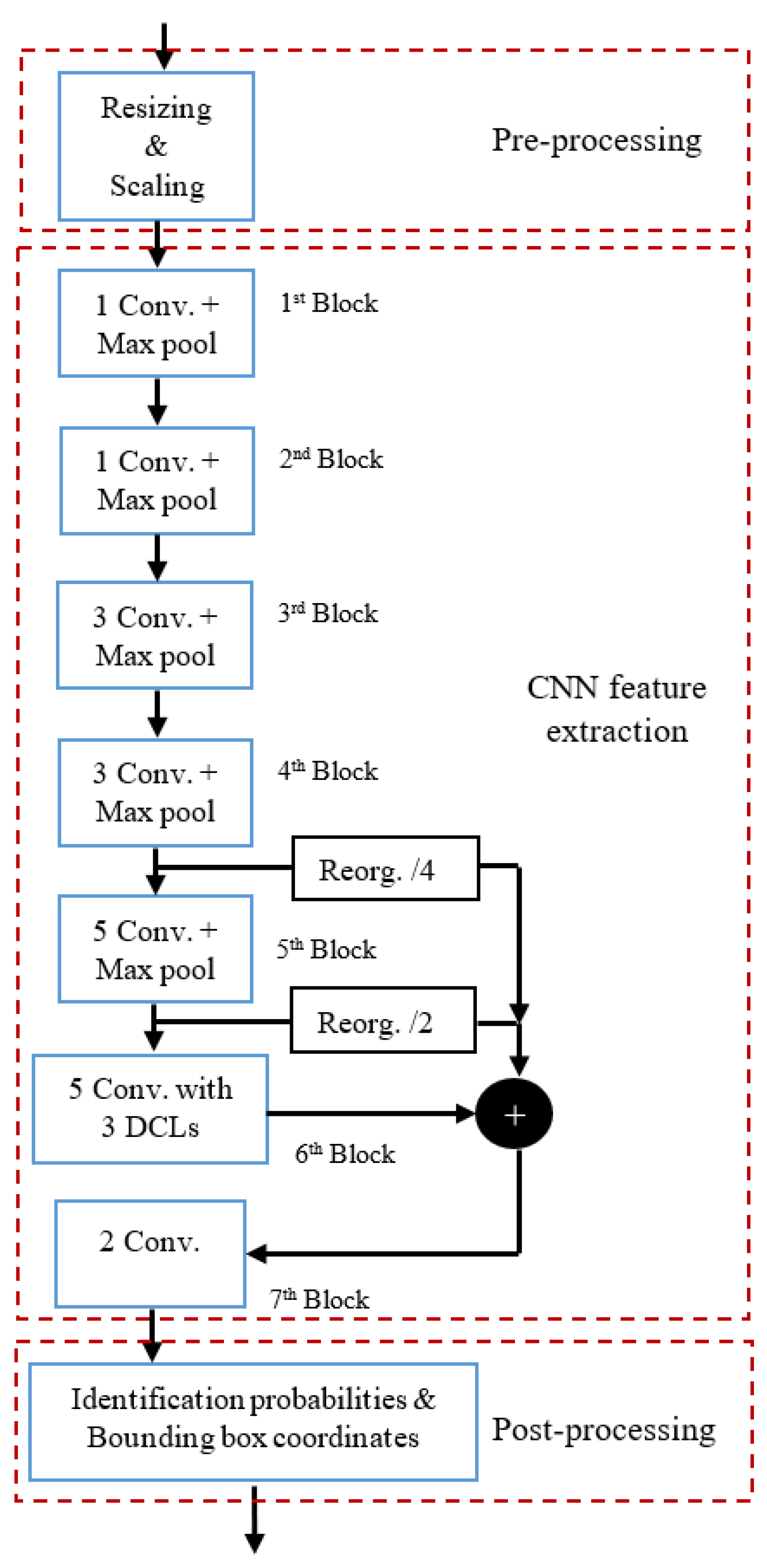
The detection model subsystem, as shown in Figure 5, consists of three sequential tasks: pre-processing, CNN feature extraction, and post-processing. Each of these tasks is implemented as a distinct function coded in Python and is executed one after the other on a single core. The CNN feature extraction task is made up of seven blocks, and each block contains multiple layers. For example, both the first and second blocks consist of two layers: a convolution layer (denoted as Conv.) and a max. pooling layer (denoted as Max pool). However, the third block contains three convolution layers and one max. pooling layer, and so forth.
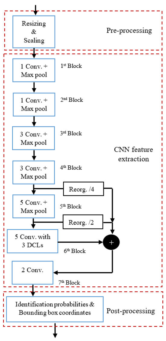
Figure 5.
Sequential processing flow of the detection model subsystem.
Measuring the processing time of each task in the detection model subsystem is crucial for reducing its processing delay. Python’s “time” module/library with the “time.time ()” function is used to measure this time on a Core i7 system [20]. The processing times of pre-processing (T1), CNN feature extraction (T2), and post-processing (T3) tasks take 1.67 ms, 20.04 ms, and 0.28 ms, respectively. Therefore, the total sequential detection processing time (Tsp) for each frame can be calculated as:
Tsp = T1 + T2 + T3
Achieving a detection processing time of 21.99 ms per frame is impressive and demonstrates enhanced detection speed. Considering the requirements of our wildlife mitigation system, especially in real-time scenarios with multiple occurrences of high-speed wildlife movements, faster processing speed is crucial. It ensures timely and accurate detection, allowing the system to respond to sudden wildlife activity and facilitate proactive mitigation. Moreover, this system is intended for deployment on a low-power embedded device. As discussed in [1], the processing time on the RP4B is 160 ms per frame for a single animal detection in portable field applications. This highlights the need for further improvements to balance detection speed and power constraints within the deployment hardware. Therefore, a parallel processing technique is proposed for the M-YOLO detector to distribute the computational workload across multiple processors or cores. This is expected to lead to faster processing of input frames and increased throughput.
5.2. Pipeline Parallelism Approach for the Detection Model
Pipeline parallelism is a computational model that allows tasks to be processed in a sequence of stages, where each stage performs a specific function and passes its output to the next stage in the pipeline [20]. This approach helps in enhancing the processing time as multiple tasks can be processed concurrently at different stages of the pipeline.
The goal of this approach, in the context of the M-YOLO model, is to balance the processing load across all pipeline stages and then execute them simultaneously [21,22]. To facilitate communication between cores/stages, shared memory is positioned between adjacent ones [23]. A combination of mutex and barrier synchronization mechanisms is employed to ensure that only one stage can access the shared memory at a time and synchronize the stages at the end of each task by reaching an appropriate synchronization point, identified as the longest processing time, before proceeding to the next frame [24]. This helps to avoid data races and corruption while ensuring orderly access to the shared memory.
In order to implement pipeline parallelism in our M-YOLO model, it is essential to go through the following process.
5.2.1. Indexing and Labeling the M-YOLO Layers
The M-YOLO model, as shown in Figure 5, is composed of several blocks operating in a sequential fashion. Each block contains a certain number of layers, leading to a cumulative total of L layers. We merge the pre-processing and post-processing tasks with the first and last convolution layers of the CNN feature extraction task, respectively.
The execution order of these L sequential layers imposes the task execution sequence. The first input layer must be evaluated based on the M-YOLO model input. Subsequently, the second layer can be evaluated once the first layer has completed executing. The model’s layers are labeled with an index i, ranging from 1 to L. The correct execution order of the L layers is:
L1 → L2 → · · · LL−1 → LL
5.2.2. M-YOLO Model Assumptions
There are some assumptions needed to pipeline the M-YOLO model, as follows:
- As mentioned before in Section 5.1, the processing time of the pre- and post-processing tasks of the M-YOLO model is small compared to that of the CNN feature extraction task. Therefore, we merge the pre-processing and post-processing tasks with the first and last convolution layers of the CNN feature extraction task, respectively, as represented by the following equations:
t1 ← t1 + Tpre
tL ← tL + Tpost
- Tpre: processing time of the pre-processing task;
- Tpost: processing time of the post-processing task;
- t1: processing time of the first convolution layer of the CNN feature extraction task;
- tL: processing time of the last convolution layer of the CNN feature extraction task.
Subsequently, for the M-YOLO model comprising L layers, the processing time of each layer of the M-YOLO model is represented by the vector T, defined as:
The total processing time of the M-YOLO model is given by:
The maximum processing time of the M-YOLO model is defined as:
Tmax = max(T)
- Merge the fifth and sixth blocks of the M-YOLO model, as in Figure 5, along with the two passthrough Reorg. (Reorganization) layers into one block, name it the ‘passthrough block’, and treat it as a single layer. This merging is performed because the passthrough layers cannot be broken down or separated without affecting the model’s performance.
5.2.3. Pipeline Throughput
The performance of the M-YOLO model is governed by the delay of the M-YOLO layers. The pipeline clock duration/period (Tclk) for the fastest pipeline is given by:
Tclk ≥ Tmax
Based on that, the throughput th of the pipeline is given by:
5.2.4. Number of Pipeline Stages in Multicore Systems
Pipeline stages can be created with as many cores as are available on the used platform to achieve higher throughput for CNN inference. However, determining the maximum number of pipeline stages is crucial as it allows for optimal resource allocation and balances the computational load, thereby enhancing the model’s processing speed.
There are several restrictions when determining the number of pipeline stages S:
- The minimum number of pipeline stages satisfies the inequality:
S > 1
- The maximum limit on the number of pipeline stages is imposed by the hardware support of the multicore system:
S ≤ C
- The number of pipeline stages, S, should be determined in a way that the total processing time across all pipeline stages is at least as long as the total processing time of the M-YOLO model, as expressed by:
S × Tclk ≥ Ttotal
After calculating the number of pipeline stages, it is vital to design and distribute the M-YOLO layers across these stages. To address this, in the subsequent section, we propose a systematic algorithm for designing pipeline stages.
5.2.5. Proposed Algorithm for Allocating Layers to Pipeline Stages
This algorithm aims to achieve a balanced distribution of computational workload by allocating the M-YOLO model layers to pipeline stages. The goal is to ensure that all stages have processing times close to a given maximum processing time, Tmax, while adhering to the specified number of pipeline stages, thereby preventing any stage from becoming a bottleneck and slowing down the overall processing speed.
The primary inputs for this algorithm are the vector T, which represents the processing time of each layer; Ttotal, which denotes the total processing time of the model; Tclk, representing the pipeline clock period; and S, the desired number of pipeline stages.
This algorithm attempts to distribute the layers across the specified number of pipeline stages, ensuring that the total processing time for each stage is within the specified pipeline clock period, Tclk. By doing so, it enhances resource utilization and thereby the processing speed of the detection model during inference, leading to a well-distributed computational load across different pipeline stages.
5.2.6. Pipelining Implementation of M-YOLO Model Using Python 3.7
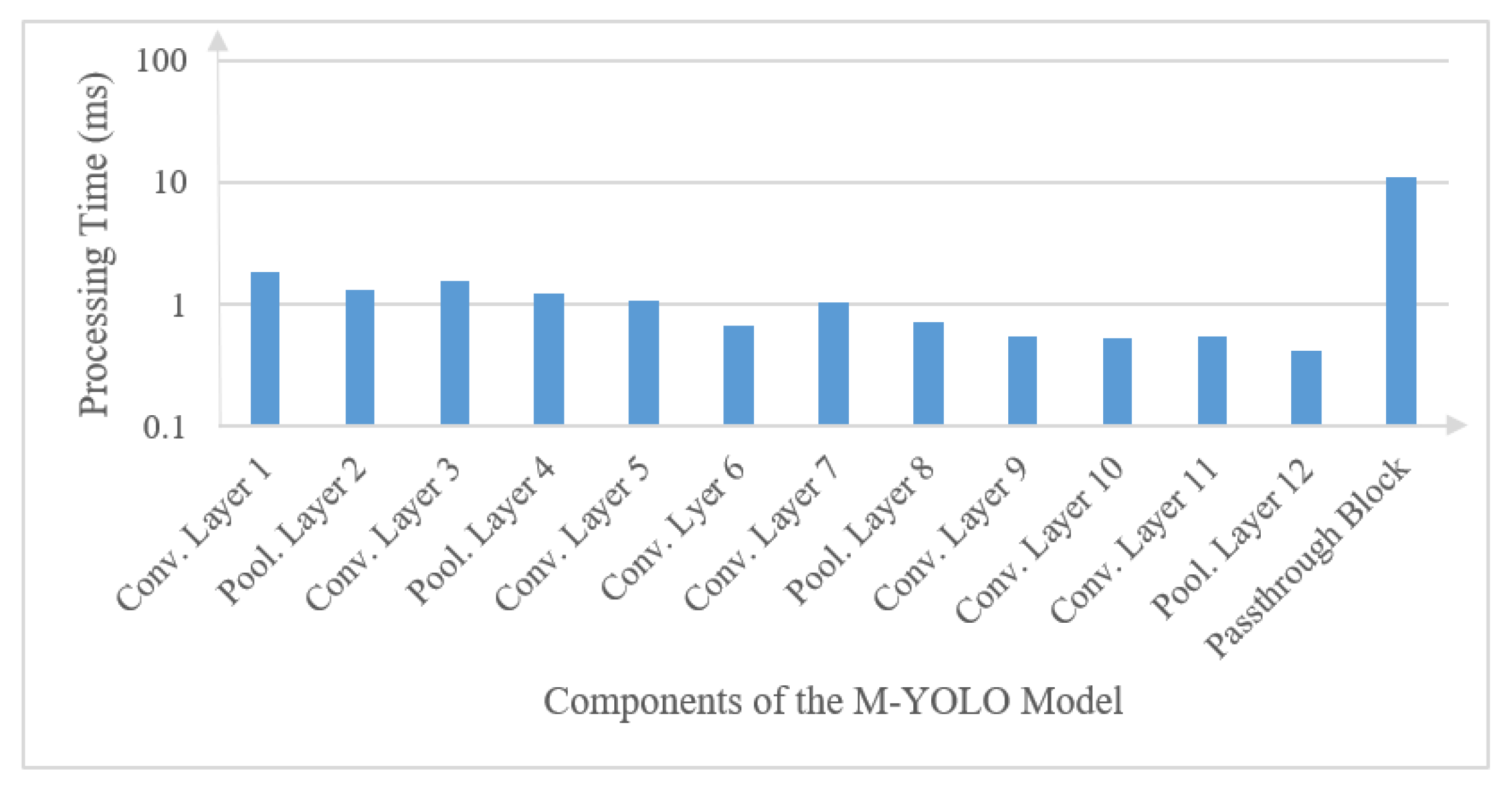
The processing time of each layer of the M-YOLO model was measured on a Core i7 system using the Python module mentioned in Section 5.1. Although the seventh block seems independent, the processing times of its convolution layers are 0.13 ms and 0.02 ms, respectively. Given these small processing times, treating it separately would make it challenging to achieve a balanced pipeline. Therefore, merging the seventh block with the fifth and sixth blocks emerges as an efficient strategy for pipeline processing. Figure 6 represents the processing time of the first 12 layers of the CNN feature extraction task and the passthrough block, which is treated as a single layer, within the M-YOLO model.
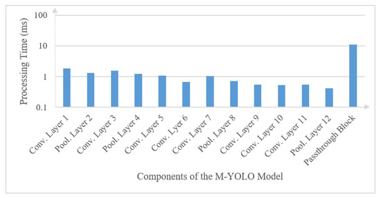
Figure 6.
Processing time for the components of the M-YOLO model as measured on a Core i7 system.
Given the structure of the M-YOLO model, the passthrough block is treated as a single layer, which provides the maximum processing time, Tmax = 11.20 ms. As mentioned in Section 5.1, the total processing time of the M-YOLO model is Ttotal = 21.99 ms. From Equation (13), and based on the restrictions outlined in Section 5.2.3, the number of pipeline stages, S, is set to 2. Therefore, a two-stage implementation is adopted for the M-YOLO model.
In the two-stage pipelining, after merging the pre-processing task to the first convolution layer and the post-processing task to the last convolution layer of the M-YOLO model, the allocation of layers to pipeline stages was performed following the proposed Algorithm 2. The first 12 layers of the M-YOLO model are assigned to the first stage, which takes a processing time of T1s = 10.79 ms. Meanwhile, the passthrough block, which is treated as a single layer, is assigned to the second stage, which takes a processing time of T2s = 11.20 ms. The constraint imposed by the passthrough layers restricts the allocation from extending beyond the first 12 layers, ensuring the integrity and functionality of the model while adhering to the pipelining paradigm.
| Algorithm 2 Proposed algorithm for allocating layers to pipeline stages. |
Require:T, , S.
|
5.3. Background of Dataflow Approach
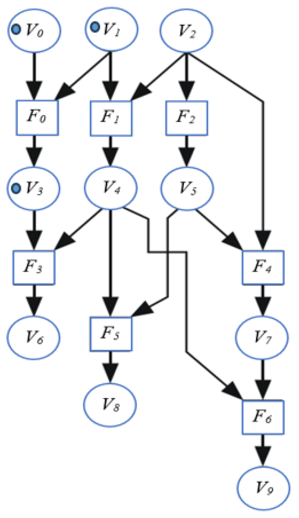
In this section, we explore how data dependencies between different tasks can be represented by a dataflow graph (DFG). This DFG consists of three sets: variables (V), functions (F), and directed arcs (A). Variables are classified into three types based on their locations in the algorithm: input, intermediate, and output. Functions represent the tasks and operations of the algorithm, and they are allocated to processors. Directed arcs depict the communication and dependencies between variables and functions, associating them with memories or registers. Figure 7 provides an example of a DFG of an algorithm composed of ten variables and seven functions [25]. Variables could have multiple outputs but only one input, while functions might have multiple inputs but only one output.
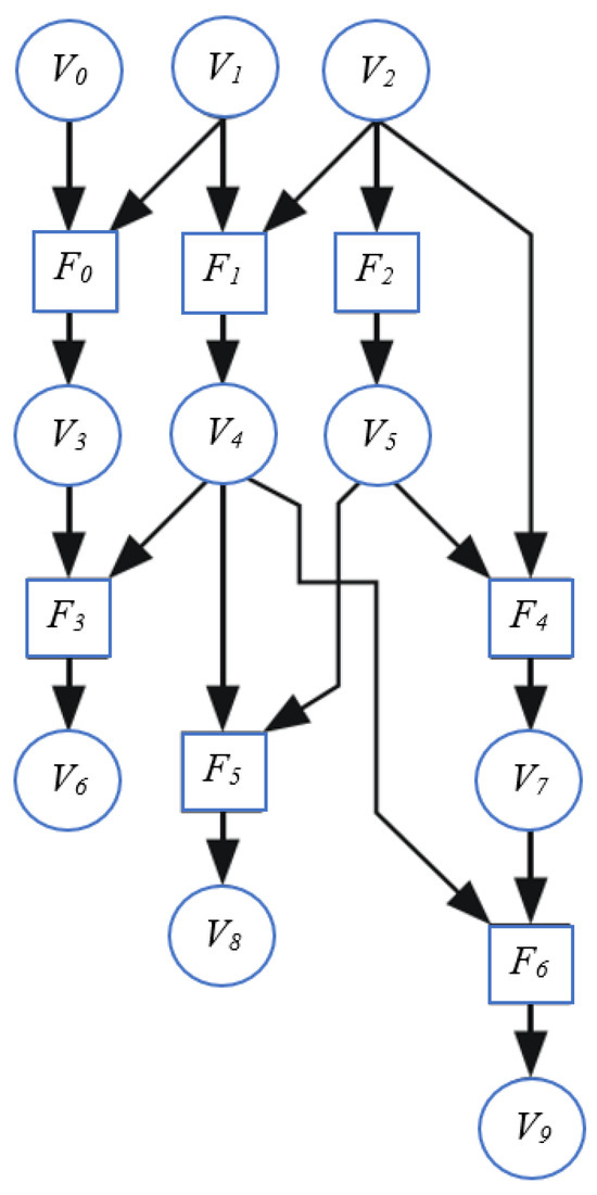
Figure 7.
A DFG for an algorithm. A variable is denoted by a circle and a function is denoted by a square.
As shown in Figure 8, the timing of the availability of variables marking the initiation of function execution is represented by blue circles on the graph, termed events/tokens. These tokens are assigned to the variables when they are valid and available for use by the function. Variables V0 and V1 have tokens, indicating that functions F0 and F1 will be triggered. Consequently, when a function is finished, a token is placed at the variable node associated with its output to signify the availability of this variable, as can be observed with the internal variable V3.
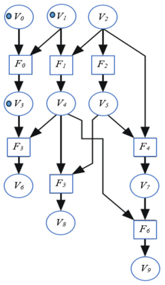
Figure 8.
State of DFG for an algorithm at a given time.
In Python, to ensure that data flow in the correct order and resources are accessed in a safe manner, synchronization mechanisms are implemented. A combination of condition-variable and mutex synchronization mechanisms is well suited for scenarios that require a flexible synchronization strategy, where individual tasks either proceed or wait based on a specific condition, rather than synchronizing all cores at a common point. This condition revolves around the availability of new data in the shared memory block.
5.4. Proposed Pipelining–Dataflow Hybrid Approach for the Detection Model
This hybrid approach aims to leverage the throughput benefits of pipelining while incorporating the data-driven execution characteristic of dataflow paradigms to manage conditional processing based on the MCF algorithm. In a pure pipelining paradigm, each pipeline stage would proceed to process data in a fixed sequence without conditional decision making based on data content. On the other hand, a pure dataflow paradigm would have tasks executed more independently based on data availability without a fixed sequence of stages.
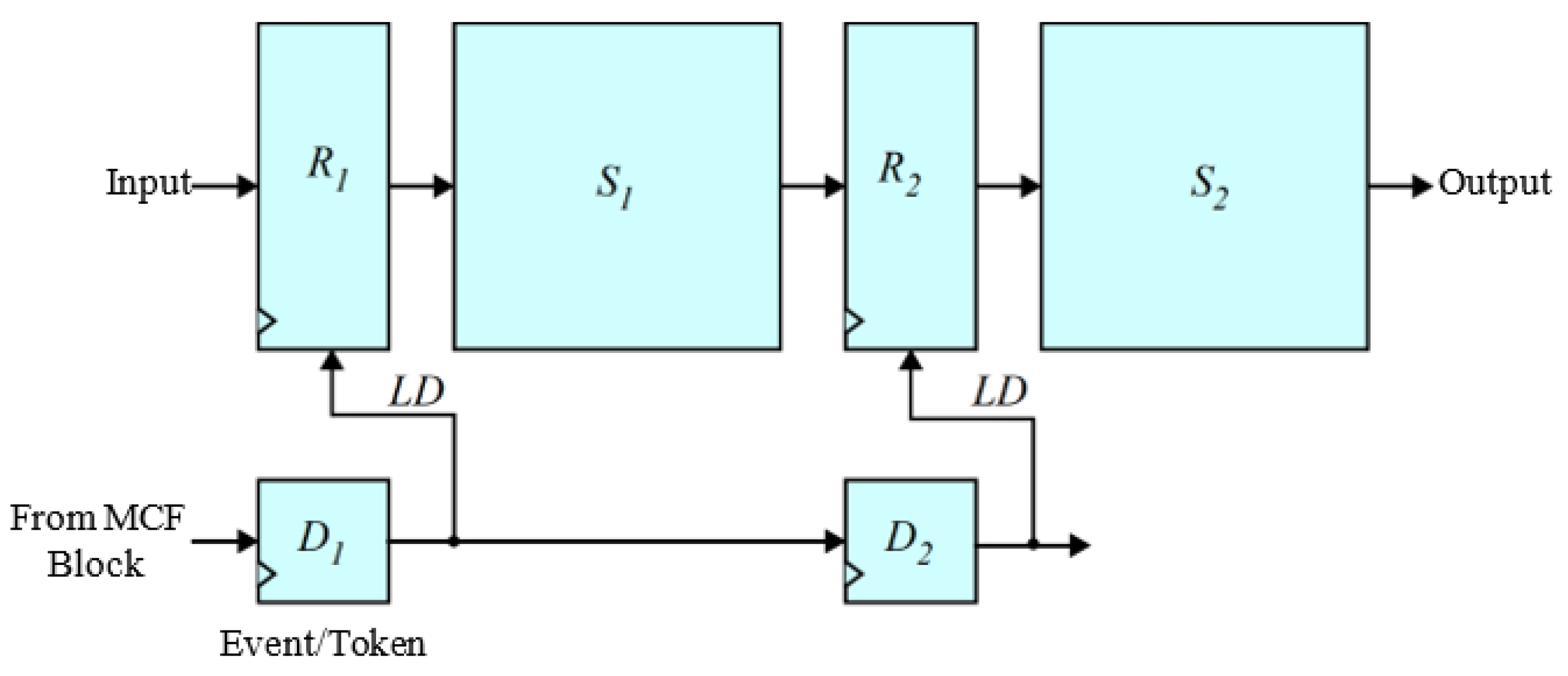
Following our experiments from Section 5.2.6, we employed a two-stage strategy to implement the pipelining–dataflow hybrid approach in the proposed M-YOLO model with the integration of the MCF algorithm, named the MCF-YOLO model. As shown in Figure 9, the pipelining–dataflow hybrid approach of our proposed MCF-YOLO model is composed of two parts:

Figure 9.
Logical block diagram of a two-stage pipelining–dataflow hybrid approach of the MCF-YOLO model.
- The pipelining part, which consists of two pipeline stages, S1 and S2, with two registers/memories R1 and R2.
- The dataflow part, which manages the data-driven conditional processing. When the MCF block identifies motion within frames, the event/token D1 signals and prompts R1 to load the data (LD). After a designated clock period, D2 signals, instructing R2 to load the data (LD) to the second processing stage, S2, which then initiates its operations.
Algorithm 3 represents the implementation of a two-stage pipelining–dataflow hybrid approach in the proposed MCF-YOLO model.
| Algorithm 3 Two-stage pipelining–dataflow hybrid paradigm for the MCF-YOLO model. |
| Create: shared memory space: shared_memory; condition variable: condition_variable; mutex: mutex_lock;
|
Algorithm 3 illustrates a hybrid approach, combining aspects of both pipelining and dataflow paradigms. Here is how:
- Pipelining: The arrangement of Stage 1, S1, and Stage 2, S2, in a fixed sequence where Stage 2 depends on the output of Stage 1 represents a pipelining paradigm. Pipelining helps in maximizing the throughput of the processing by allowing Stage 2 to process one frame while Stage 1 is processing the next.
- Dataflow: The use of a condition variable to synchronize the processing of pipeline stages based on the availability of data (in this case, motion detected, and data readiness signaled by a token) represents a dataflow paradigm. In dataflow, the execution of pipeline stages is driven by data availability.
- Conditional Processing: The conditional processing based on motion detection is a characteristic of data-driven processing, which is a key aspect of dataflow paradigms.
- Shared Memory: The use of shared memory for inter-stage communication is a common technique in both pipelined and dataflow architectures to enable data sharing between different stages or processes. The mutex is used to prevent data corruption during concurrent access by the two stages.
The integration of a decision node (motion detection/MCF algorithm) to direct the flow of data, coupled with synchronization based on data availability (signaled by a condition variable), blends elements of both pipelining and dataflow paradigms. This hybrid approach aims to leverage the throughput benefits of pipelining while incorporating the data-driven execution characteristic of dataflow paradigms to manage conditional processing based on motion detection.
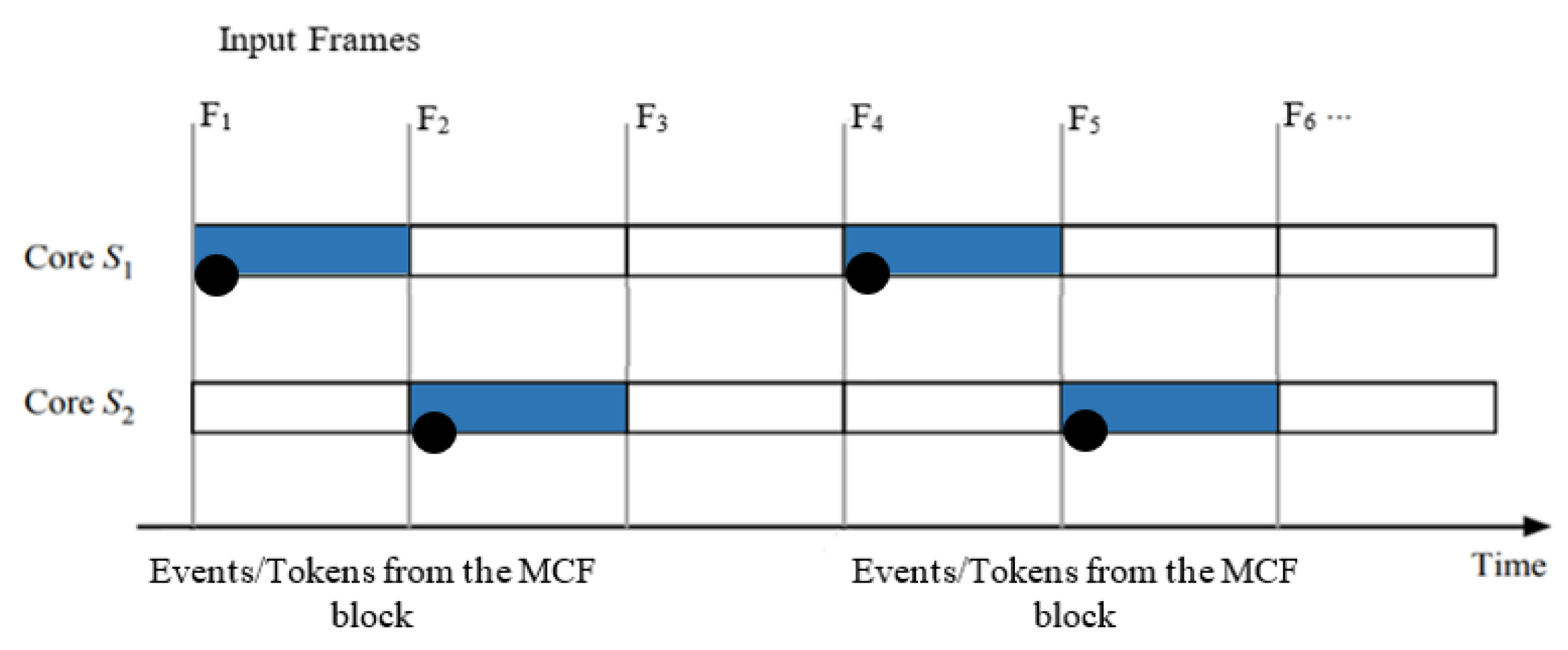
Figure 10 shows an example of the two-stage pipelining–dataflow hybrid approach of the MCF-YOLO model. When a frame exhibits motion, an event/token, denoted by a black circle, triggers the first stage, S1, to process the first 12 layers of the CNN feature extraction task. Subsequently, after a pipeline clock period another event/token, denoted by a black circle, triggers the second stage, S2, to process the passthrough block of the MCF-YOLO model. Among the frames, F1 and F4 exhibit motion, while F2, F3, F5, and F6 do not.

Figure 10.
Parallel implementation of the MCF-YOLO model using two-stage pipelining–dataflow hybrid approach. Data transfer time is insignificant.
6. Efficiency Evaluation of the MCFP-YOLO Detector: Processing Speed and Power Consumption
By parallelizing the MCF-YOLO detector using the two-stage pipelining–dataflow hybrid approach, we produced a new detector named MCFP-YOLO, as shown in Figure 11. The evaluation metrics provide valuable information on the efficiency and effectiveness of the proposed MCFP-YOLO animal species detector in real-world scenarios. Efficiency refers to achieving our goals with minimal processing time and power consumption; while effectiveness refers to the detector’s ability to accurately identify and localize objects in images, as well as its proficiency in distinguishing between various classes, even with subtle differences between them.
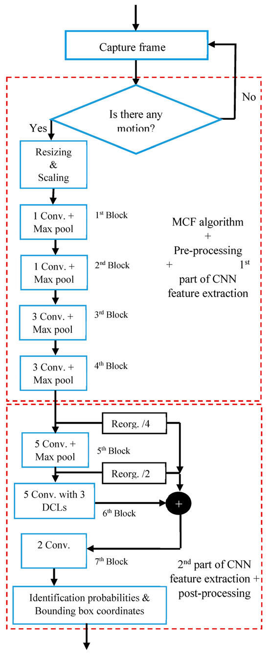
Figure 11.
Processing flow of the M-YOLO model after integrating the MCF algorithm and two-stage pipelining–dataflow hybrid approach.
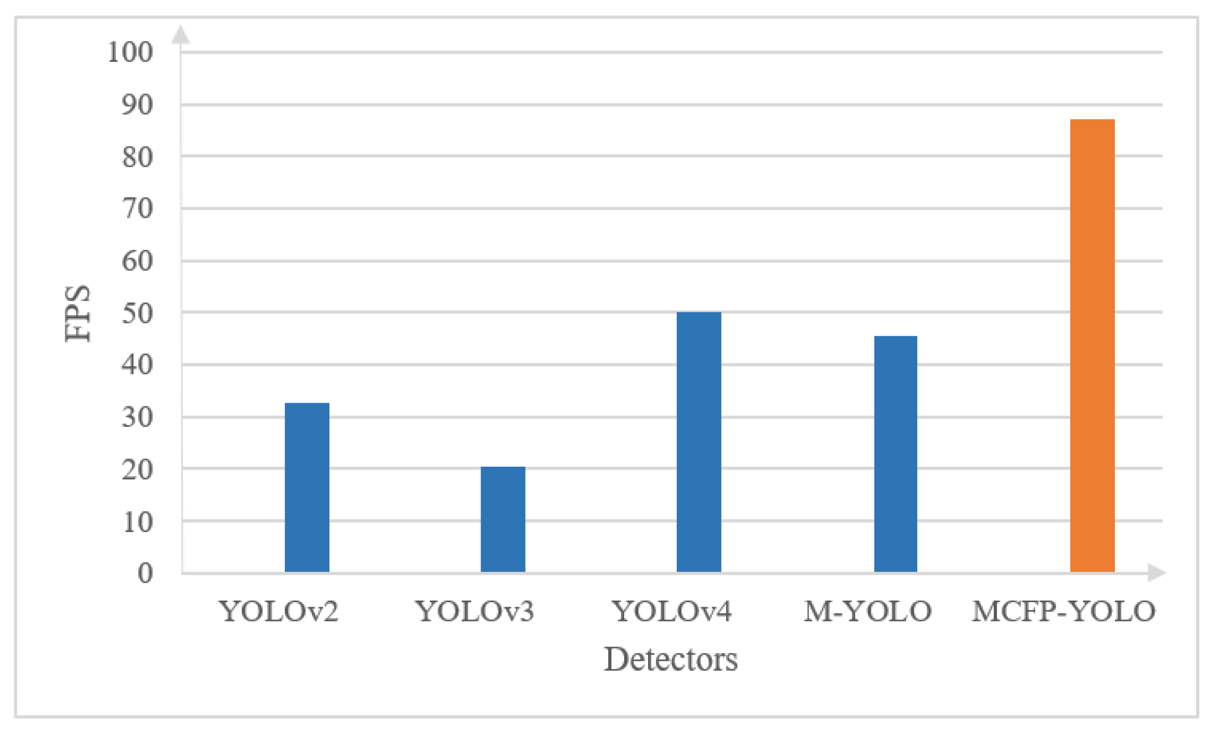
Figure 12 and Figure 13 present a comparison, carried out on a Core i7 system, between the proposed MCFP-YOLO (MCF-YOLO with parallel processing) and the original M-YOLO detector, as well as YOLOv2, YOLOv3, and YOLOv4 in terms of the elapsed time and FPS for batch processing and real-time processing [1], respectively. As shown in Figure 11, for batch processing of a 4160-frame video with a resolution of 1280 × 720 pixels, sourced from [26] in which 69% of the frames exhibit motion, the elapsed time of the proposed MCFP-YOLO detector is markedly less than that of the other models. It shows a 66.5% reduction in elapsed time compared to the original M-YOLO detector, and reductions of 88.7%, 86.1%, and 87.4% compared to YOLOv2, YOLOv3, and YOLOv4, respectively. The enhanced processing time of the MCFP-YOLO is attributed to its selective frame processing strategy, which processes only the frames with motion using parallel computation, thereby enhancing the computational workload and reducing the time required for processing extensive video datasets. Similarly, as shown in Figure 12, for real-time processing using footage from a 30 FPS web camera with a resolution of 1280 × 720 pixels, the FPS of the proposed MCFP-YOLO detector is enhanced by 2.6 times compared to the original M-YOLO detector and exhibits significant improvements over YOLOv2, YOLOv3, and YOLOv4. MCFP-YOLO achieves an FPS nearly three times higher than that of YOLOv2, approximately seven times that of YOLOv3, and over two times the FPS of YOLOv4, indicating its superior performance in real-time scenarios.
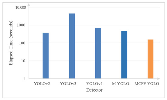
Figure 12.
Processing speed comparison of various object detection models and the proposed MCFP-YOLO animal species detector in terms of elapsed time for batch processing sourced from [20].
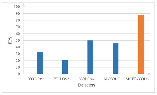
Figure 13.
Processing speed comparison of various object detection models and the proposed MCFP-YOLO animal species detector in terms of FPS for real-time processing from a web camera feed.
Following the demonstration of the enhanced processing speed with the proposed MCFP-YOLO, the CPU utilization metric [27] is used to evaluate and compare the power consumption of the CPU during the operation of various object detection models in batch and real-time processing. As shown in Figure 14, for batch processing, YOLOv4 has the highest CPU utilization, indicating a more intensive computational requirement, while MCFP-YOLO shows a significant decrease in utilization, suggesting improved efficiency in terms of power consumption. During real-time processing, YOLOv4 again peaks in CPU usage, but MCFP-YOLO maintains a lower and more consistent utilization, reinforcing its suitability for applications with limited power resources or those requiring longer operational durations without compromising detection accuracy. This reduction in power consumption of the MCFP-YOLO model is achieved because the CPU enters idle states during periods when frames are dropped due to the absence of detected animal motion. Furthermore, the two-stage pipelining–dataflow hybrid approach contributes to power savings by allowing for more efficient use of cores and reducing idle time.
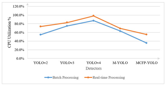
Figure 14.
Comparison of CPU utilization percentage for various object detection models and the proposed MCFP-YOLO animal species detector using batch processing sourced from [20] and real-time processing from a web camera feed.
The above results emphasize the advantages of the proposed MCFP-YOLO detector, making it suitable for deployment on embedded systems for WHC and WVC mitigation systems.
7. The MCFP-YOLO Detector on Embedded Systems
The proposed MCFP-YOLO detector was deployed on both the RP4B and NVIDIA Jetson Nano devices [28] to evaluate its efficiency in terms of processing speed and power consumption. This evaluation was conducted using FPS, current consumption (mA), and CPU utilization (%) metrics for real-time processing from a web camera feed.
The RP4B features a Quad-core Cortex-A72 64-bit, 1.5 GHz CPU, and a VideoCore VI 3D 500 MHz GPU. It can support up to 8 GB of SDRAM and uses a microSD for storage. RP4B has a two-lane camera port, HDMI and Display Port, and four USB ports. Additionally, the RP4B supports Gigabit Ethernet, Bluetooth 5.0, and 2.4/5 GHz Wi-Fi for connectivity [29]. Similarly, the NVIDIA Jetson Nano, another embedded device, includes a Quad-core Cortex A-57 64-bit, 1.43 GHz CPU, and an NVIDIA 128-core GPU. The Jetson Nano has 4 GB memory with a RAM speed of 25.6 GB/s and a microSD for storage. It also has a two-lane camera port, HDMI and Display Port, and five USB ports [28].
As presented in Table 1, the results show that the Jetson Nano outperforms the RP4B by approximately 1.2 times in terms of processing speed, but it also consumes approximately 4.7% more current and exhibits 33.3% higher CPU utilization. Moreover, in terms of cost, the Jetson Nano device is significantly pricier than the RP4B.

Table 1.
Comparison between RP4B and Jetson Nano devices in terms of FPS, current consumption, and CPU utilization percentage for real-time processing from a web camera feed, and cost.
Despite these differences, the RP4B device proves to be a suitable choice for our work as it offers a desirable balance between cost and efficiency, including processing speed and power consumption. Compared to other embedded devices such as those referenced in [30,31], the RP4B provides a relatively powerful processing capability at a lower cost and with less power consumption. This makes it an affordable and power-efficient option for real-time wildlife detection systems. These features enable efficient real-time processing while maintaining budget and power constraints, which are crucial for the widespread and successful deployment of WHC and WVC mitigation systems.
8. Conclusions
In this paper, we explored the integration of two ideas into the M-YOLO animal species detector: the MCF algorithm and the utilization of parallel processing technique. The MCF algorithm is designed to minimize the processing delay of the frame capture subsystem by controlling the number of frames to be processed by the detection model subsystem based on detected motion activity in the frames. On the other hand, the parallel processing technique aims to minimize the processing delay of the detection model subsystem by processing the three tasks (pre-processing, CNN feature extraction, and post-processing) in parallel using two-stage pipelining–dataflow hybrid approach. Experimental results were provided to validate these proposed ideas and their effectiveness in improving the efficiency (detection speed and power consumption) of the proposed MCFP-YOLO detector, particularly for embedded systems with limited resources.
The proposed MCFP-YOLO detector was then deployed on both RP4B and Jetson Nano devices to assess their performance in real-life scenarios. The results indicate that while Jetson Nano outperforms the RP4B by approximately 1.2 times in terms of speed. It also consumes around 4.7% more current consumption and utilizes 33.3% more CPU. The RP4B is advantageous for our system, especially when it operates for extended durations on limited power resources, such as in remote areas or when relying on battery power. Therefore, the RP4B remains a suitable choice for wildlife detection applications due to its balance between cost and performance, making it an affordable and power-efficient option for real-time WHC and WVC mitigation systems.
Pipelining indeed shows promise in our current context, but its effectiveness may vary with different models, largely depending on their architecture.
Author Contributions
Conceptualization, M.I., K.F.L. and F.G.; methodology, M.I., K.F.L. and F.G.; validation, M.I.; investigation, M.I., K.F.L. and F.G.; writing—original draft preparation, M.I.; writing—review and editing, K.F.L. and F.G.; supervision, K.F.L. and F.G. All authors have read and agreed to the published version of the manuscript.
Funding
This research received no external funding.
Data Availability Statement
Data is contained within the article.
Acknowledgments
We gratefully acknowledge the support of the British Columbia Ministry of Transportation and Infrastructure.
Conflicts of Interest
The authors declare that there is no conflict of interest regarding the publication of this paper.
References
- Ibraheam, M.; Li, K.F.; Gebali, F. An Accurate and Fast Animal Species Detection System for Embedded Devices. IEEE Access 2023, 11, 23462–23473. [Google Scholar] [CrossRef]
- Wang, Y.; Zhou, J.; Zhang, C.; Luo, Z.; Han, X.; Ji, Y.; Guan, J. Bird Object Detection: Dataset Construction, Model Performance Evaluation, and Model Lightweighting. Anim. J. 2023, 13, 2924. [Google Scholar] [CrossRef] [PubMed]
- Adami, D.; Ojo, M.O.; Giorando, S. Design, Development and Evaluation of an Intelligent Animal Repelling System for Crop Protection Based on Embedded Eged-AI. IEEE Access 2021, 9, 132125–132139. [Google Scholar] [CrossRef]
- Sato, D.; Zanella, A.J.; Costa, E.X. Computational classification of animals for a highway detection system. Braz. J. Vet. Res. Anim. Sci. 2021, 58, e174951. [Google Scholar] [CrossRef]
- Kim, Y.-D.; Park, E.; Yoo, S.; Choi, T.; Yang, L.; Shin, D. Compression of Deep Convolutional Neural Networks for Fast and Low Power Mobile Applications. ICLR 2016, 1–16. [Google Scholar] [CrossRef]
- Li, Z.H.; Meng, L. Model Compression for Deep Neural Networks: A Survey. Computers 2023, 12, 60. [Google Scholar] [CrossRef]
- Wu, R.-T.; Singla, A.; Jahanshahi, M.R.; Bertino, E.; Ko, B.J.; Verma, D. Pruning deep convolutional neural networks for efficient edge computing in condition assessment of infrastructures. Comput. Aided Civ. Infrastruct. Eng. 2019, 34, 774–789. [Google Scholar] [CrossRef]
- Tonellotto, N.; Gotta, A.; Nardini, F.M.; Gadler, D.; Silvestri, F. Neural network quantization in federated learning at the edge. Inf. Sci. 2021, 575, 417–436. [Google Scholar] [CrossRef]
- Zhao, Y.; Wang, D.; Wang, L. Convolution Accelerator Designs Using Fast Algorithms. Algorithms 2019, 12, 112. [Google Scholar] [CrossRef]
- Cambuim, L.; Barros, E. FPGA-Based Pedestrian Detection for Collision Prediction System. Sensors 2022, 22, 4421. [Google Scholar] [CrossRef] [PubMed]
- Minakova, S.; Tang, E.; Stefanov, T. Combining Task- and Data-Level Parallelism for High-Throughput CNN Inference on Embedded CPUs-GPUs MPSoCs. In Proceedings of the International Conference on Embedded Computer Systems, Samos, Greece, 5–9 July 2020. [Google Scholar]
- Tao, H. A label-relevance multi-direction interaction network with enhanced deformable convolution for forest smoke recognition. Expert Syst. Appl. 2024, 236, 121383. [Google Scholar] [CrossRef]
- Tao, H.; Duan, Q.; Lu, M.; Hu, Z. Learning discriminative feature representation with pixel-level supervision for forest smoke recognition. Pattern Recognit. 2023, 143, 109761. [Google Scholar] [CrossRef]
- Tao, H.; Duan, Q.; An, J. An Adaptive Interference Removal Framework for Video Person Re-Identification. IEEE Trans. Circuits Syst. Video Technol. 2023, 33, 5148–5159. [Google Scholar] [CrossRef]
- Yahya, A.A.; Tan, J.; Hu, M. A novel video noise reduction method based on PDE, adaptive grouping, and thresholding techniques. J. Eng. 2021, 2021, 605–620. [Google Scholar] [CrossRef]
- Said, K.A.M.; Jambek, A.B.; Sulaiman, N. A Study of Image Processing Using Morphological Opening and Closing Processes. Int. J. Control. Theory Appl. 2017, 9, 15–21. [Google Scholar]
- Murray, P.; Marshall, S. A Review of Recent Advances in the Hit-or-Miss Transform. Adv. Electron. Electron Phys. 2013, 175, 221–282. [Google Scholar]
- Bovik, A. Handbook of Image and Video Processing; Academic Press: Cambridge, MA, USA, 2010. [Google Scholar]
- Rawat, P.; Sawale, M.D. Gaussian kernel filtering for video stabilization. In Proceedings of the 2017 International Conference on Recent Innovations in Signal Processing and Embedded Systems (RISE), Bhopal, India, 27–29 October 2017. [Google Scholar]
- Dell G3. 15 Setup and Specification. August 2019. Available online: https://dl.dell.com/topicspdf/g-series-15-3579-laptop_users-guide_en-us.pdf (accessed on 24 May 2022).
- Wang, S.; Ananthanarayanan, G.; Zeng, Y.; Goel, N.A.; Mitra, T. High-Throughput CNN Inference on Embedded ARM Big.Little Multicore Processors. IEEE Trans. Comput. -Aided Des. Integr. Circuits Syst. 2020, 39, 2254–2267. [Google Scholar] [CrossRef]
- Alazahrani, A.; Gebali, F. Multi-Core Dataflow Design and Implementation of Secure Hash Algorithm-3. IEEE Access 2018, 6, 6092–6102. [Google Scholar] [CrossRef]
- Silberschatz, A.; Galvin, P.B.; Gagne, G. Operating System Concepts, 10th ed.; John Wiley & Sons: Hoboken, NJ, USA, 1991. [Google Scholar]
- Stuart, J.A.; Owens, J.D. Efficient Synchronization Primitives for GPUs. arXiv 2011, arXiv:1110.4623v1. [Google Scholar]
- Alazahrani, A.; Gebali, F. Dataflow Implementation of Concurrent Asynchronous Systems. In Proceedings of the IEEE Pacific Rim Conference on Communication, Computers and Signal Processing (PACRIM), Victoria, BC, Canada, 21–23 August 2017; pp. 1–5. [Google Scholar]
- WATCH: Trio of Cougars Spotted in British Columbia Backyard. CTV News. February 2023. Available online: https://www.youtube.com/watch?v=4sdWeiyWZ0w&t=6s (accessed on 25 February 2023).
- Chekkilla, A.G.; Kalidindi, R.V. Monitoring and Analysis of CPU Utilization, Disk Throughput and Latency in Servers Running Cassandra Database; Faculty of Computing, Blekinge Institute of Technology: Karlskrona, Sweden, 2016. [Google Scholar]
- Getting Started with Jetson Nano Developer Kit. Nvidia Developer. Available online: https://developer.nvidia.com/embedded/learn/get-started-jetson-nano-devkit (accessed on 11 April 2023).
- Raspberry Pi. Available online: https://www.raspberrypi.com/products/raspberry-pi-4-model-b/ (accessed on 8 December 2021).
- Nvidia. Embedded Systems with Jeston. Available online: https://www.nvidia.com/en-us/autonomous-machines/embedded-systems/ (accessed on 6 April 2023).
- Intel. Intel Products. Available online: https://www.intel.com/content/www/us/en/products/overview.html (accessed on 6 April 2023).


Disclaimer/Publisher’s Note: The statements, opinions and data contained in all publications are solely those of the individual author(s) and contributor(s) and not of MDPI and/or the editor(s). MDPI and/or the editor(s) disclaim responsibility for any injury to people or property resulting from any ideas, methods, instructions or products referred to in the content. |
© 2023 by the authors. Licensee MDPI, Basel, Switzerland. This article is an open access article distributed under the terms and conditions of the Creative Commons Attribution (CC BY) license (https://creativecommons.org/licenses/by/4.0/).