Abstract
Video salient object detection has attracted growing interest in recent years. However, some existing video saliency models often suffer from the inappropriate utilization of spatial and temporal cues and the insufficient aggregation of different level features, leading to remarkable performance degradation. Therefore, we propose a quality-driven dual-branch feature integration network majoring in the adaptive fusion of multi-modal cues and sufficient aggregation of multi-level spatiotemporal features. Firstly, we employ the quality-driven multi-modal feature fusion (QMFF) module to combine the spatial and temporal features. Particularly, the quality scores estimated from each level’s spatial and temporal cues are not only used to weigh the two modal features but also to adaptively integrate the coarse spatial and temporal saliency predictions into the guidance map, which further enhances the two modal features. Secondly, we deploy the dual-branch-based multi-level feature aggregation (DMFA) module to integrate multi-level spatiotemporal features, where the two branches including the progressive decoder branch and the direct concatenation branch sufficiently explore the cooperation of multi-level spatiotemporal features. In particular, in order to provide an adaptive fusion for the outputs of the two branches, we design the dual-branch fusion (DF) unit, where the channel weight of each output can be learned jointly from the two outputs. The experiments conducted on four video datasets clearly demonstrate the effectiveness and superiority of our model against the state-of-the-art video saliency models.
1. Introduction
Video salient object detection aims to highlight the most visually attractive objects in videos, leading to the filtering of the irrelevant video contents. Thus, video salient object detection has been widely applied to many related areas, such as abnormal event detection [1], gait recognition [2], video image compression [3,4], car detection [5], to name a few. Different from the image salient object detection [6,7,8], video salient object detection should consider the spatial and temporal cues simultaneously. Particularly, the spatial information of each frame is often polluted by the cluttered background or low contrast between salient regions and background, and while the temporal information embedded in different frames is easily disturbed by the fast motion and large displacement scene. This makes the difficulty of video salient object detection greater than that of image salient object detection.
In recent years, with the remarkable development of deep learning techniques, the performance of video saliency models [9,10,11,12,13,14,15,16,17,18,19,20,21] is pushed forward significantly. Generally, the existing video saliency models try to acquire the temporal dynamic information via traditional convolutional neural networks [9,10], ConvLSTM [11,12], 3D convolutional neural networks [13,14], and optical flow [19,20,21]. Among these efforts, we notice that the optical flow-based models are usually organized in a two-stream structure, but their performance may be largely hindered by the low-quality optical flow image. In particular, some two-stream models either treat the two modal features equally or rely heavily on the temporal cues, which ignores the inherent differences between spatial and temporal information. Interestingly, we find that some efforts [17,22,23] utilize quality scores to evaluate the reliability of different modal features, which provides a good reference for the future efforts. Moreover, in the decoding process of the existing video saliency detection networks [9,21], they either adopt the U-shaped architecture or choose the fully convolutional neural networks, which usually overlook the disparity of the effects of different level deep features and give insufficient aggregation of multi-level deep features. To remit this dilemma, some methods attempt to adopt a dual-branch structure [24,25,26,27], adjacent layer integration [8], multi-resolution based fusion [28], and vision-transformer-based fusion [29,30,31] to promote the fusion of multi-level deep features.
Motivated by the aforementioned analysis, we present a quality-driven dual-branch feature integration network shown in Figure 1, where the two key components are the quality-driven multi-modal feature fusion (QMFF) module and the dual-branch-based multi-level feature aggregation (DMFA) module. Specifically, we first introduce quality score estimation [17] into our QMFF module. However, different from [17], the quality scores in the QMFF module are not only employed to re-calibrate spatial and temporal features, but also treated as weights to fuse the coarse saliency predictions of the two modal features into the guidance map. Particularly, the QMFF module further employs the guidance map to steer the re-calibrated features to give more attention to salient regions. After that, the QMFF module fuses the enhanced spatial and temporal features into spatiotemporal features. In this way, the QMFF module effectively explores the complementarity of the two modal features.
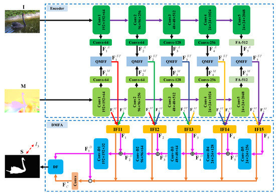
Figure 1.
The architecture of the proposed video saliency model: the inputs are current frame image and its optical flow image . Firstly, the encoder network is employed to generate the appearance features and the motion features . Then, the two modal features are combined by the quality-driven multi-modal feature fusion (QMFF) module, yielding the multi-level spatiotemporal deep features . Next, we deploy the inter-level feature interaction (IFI) unit on each level spatiotemporal feature to obtain the enhanced spatiotemporal features . After that, we deploy the dual-branched-based multi-level feature aggregation (DMFA) module to integrate the spatiotemporal features, yielding deep decoding features and concatenation features . Successively, we use the dual-branch fusion (DF) unit to integrate the two features including and , generating the final high-quality saliency map . Here, is the supervision.
Moreover, we deploy the DMFA module to sufficiently aggregate the multi-level spatiotemporal features. Similar to [8], the DMFA module first employs the inter-level feature interaction (IFI) unit to elevate the spatiotemporal features by introducing the adjacent level features. Then, inspired by [24], the DMFA module introduces the dual-branch decoders consisting of the progressive decoder branch and the direct concatenation branch to adequately utilize the multi-level features, which digs main body and local details of salient objects simultaneously. Different from [24], we further design the dual-branch fusion (DF) unit to integrate the two branches’ outputs, where channel weights are learned to adaptively re-calibrate the two outputs. In this way, our model can effectively highlight salient objects in videos.
Overall, the main contributions of this paper can be summarized as follows:
- We propose a quality-driven dual-branch feature integration network, consisting of the quality-driven multi-modal feature fusion (QMFF) module and the dual-branch-based multi-level feature aggregation (DMFA) module, to appropriately and sufficiently utilize multi-modal and multi-level features.
- We design the QMFF module to sufficiently explore the complementarity of the spatial and temporal features, where the quality scores are treated as weights to re-calibrate the two modal features and generate the guidance map. Particularly, the guidance map steers the two modal features to pay more attention to salient regions.
- We deploy the DMFA module to adequately integrate the multi-level spatiotemporal features, where the dual-branch fusion (DF) unit is designed to fuse the outputs of two branches including the main body cues of progressive decoder branch and the local details of direct concatenation branch.
2. Related Works
2.1. Handcrafted-Feature Based Video Saliency Models
The traditional video saliency models are usually built based on the handcrafted features. For example, in [32], the intra-frame boundary cues and the inter-frame motion cues based gradient flow field and the graph-based energy optimization are combined to the spatiotemporal saliency maps. After that, Wang et al. [33] employed spatial edge feature and temporal motion boundary features to compute the geodesic distances which provide the coarse saliency estimation. In [34], Zhou et al. utilized an ensembling regressor to map the regions’ color, location, motion, and texture features to saliency scores. Fang et al. [35] fused the spatial and temporal information by uncertainty weight. In [36], the dual-graph-based structure is deployed to acquire saliency maps by utilizing the spatiotemporal background priors, which can be computed by SIFT features. In [37], the spatiotemporal-constrained optimization model regards saliency detection as graph propagation, which consists of the color feature-based foreground potential, background potential, smoothness potential, and the local constraint. In [38], the random walk with restart is used to integrate the spatial and temporal features which contain motion distinctiveness, temporal consistency, abrupt change, intensity, color, and compactness. Different from the existing graph-based models, Li et al. [39] utilized the kernel regression-based hybrid fusion method to combine the spatial and temporal saliency. Chen et al. [40] utilized the spatiotemporal low-rank coherency to guarantee the temporal saliency consistence among frames. Moreover, in [41], the bi-level Markov Random Field method is proposed to suitably embed the spatiotemporal consistency into the semantic labels. In [42], the inter-frame similarity and the inter-frame similarity matrices are computed to serve the temporal and spatial saliency propagation. Especially, in [43], the local estimation model, where a random forest regressor is trained within a local temporal window, together with the spatiotemporal refinement step they are used to elevate the saliency prediction. In [44], object-level saliency cues based proposal ranking and voting strategy is deployed to filter non-salient regions and choose salient regions. Similarly, in [45], the multi-cue integration framework is deployed to combine various saliency cues and achieves temporal consistency.
Different from the existing handcrafted-feature-based video saliency models, we build our video saliency model based on the deep learning technology (i.e., convolutional neural networks), where the proposed quality-driven dual-branch feature integration network gives a good representation for salient objects in videos.
2.2. Deep Learning-Based Video Saliency Models
In recent years, deep learning technology has also been applied in video salient object detection. For example, in [9], Wang et al. deployed the dynamic saliency model which incorporates the static saliency prediction to perform the spatiotemporal saliency estimation. In [19], the temporal consistence is enhanced by utilizing optical flow-based motion information and the appearance cues. In [10], the step-gained fully convolutional network is proposed to fuse the time axis’ memory cues and the space axis’ motion cues. In [46], the efficient multi-frame reasoning is performed by the graph cut, where the graph is built based on the estimated background and instance embedding. In [20], Li et al. proposed a two-stream video saliency model consisting of appearance branch and motion branch, where the motion-guided attention module uses the motion saliency cues to elevate the appearance sub-network. In [47], the symmetrical network is used to acquire and fuse the multi-level deep appearance and motion features. In the two-stream architecture [21], the appearance features are elevated by the temporal modulator which transfers each level motion cue to the appearance branch. In [48], Li et al. deployed a novel fine-tune strategy to retrain the pretrained image saliency model by using the newly sensed and coded temporal cues. In [49], a lightweight temporal unit is employed to endow the spatial decoder with effective temporal cues by using 3D convolutions and shuffle scheme. In [18], the dynamic context-sensitive filtering network gives more concern on the dynamic evolutions and the interaction of temporal and spatial cues. In [15], a set of constrained self-attention operations are organized in a pyramid architecture, which is used to obtain the affinity-based motion information. In [17], the confidence-guided adaptive gate module is designed to evaluate the quality of spatial and temporal features. In [50], Xu et al. proposed a graph convolutional neural network-based multi-stream architecture to conduct video salient object detection.
Moreover, the weakly supervised learning strategy has also been deployed to video salient object detection. In [51], the fused saliency map based pseudo-labels together with the limited manually labeled data which were used to train the weakly supervised spatiotemporal cascade video saliency model. In [52], the optical flow-based pseudo-labels together with the parts of manual annotations are used to train the video saliency model for precise contrast inference and coherence enhancement. Furthermore, the 3D convolutional neural networks have also been applied to video salient object detection. For example, in [53], the local and global context information is used to generate spatiotemporal deep features, which are then mapped to saliency scores by the spatiotemporal conditional random field. In [54], the spatiotemporal saliency model and the stereoscopic saliency aware model are used to capture the spatiotemporal features and the depth and semantic features, respectively. In [14], the 3D convolution-based X-shape structure is used to acquire the motion information in successive video frames. In addition, there are some models that attempt to use ConvLSTM to extract dynamic temporal cues. For example, in [11], the deeper bidirectional ConvLSTM, where the forward and backward ConvLSTM units are organized in a cascaded way, is proposed to capture the effective spatiotemporal deep features. In [12], the saliency shift is incorporated into the modeling of the dynamic temporal evolution, where the shift attention is deployed to weigh the hidden state of ConvLSTM.
Furthermore, we notice that there are some methods that attempt to use vision-transformer-based fusion strategy [29,30,31] to aggregate different-modal and different-level features. In [29], a triplet transformer network is designed to aggregate the RGB features and depth features via the depth purification module. In [30], a transformer-based cross-modality fusion network is deployed to conduct RGB-D and RGB-T salient object detection. In [31], a vision-transformer-based cross-modal fusion framework is employed to conduct RGB-X semantic segmentation, where X refers to depth, thermal, polarization, and event information.
Different from the existing deep learning-based video saliency models, our model pays more attention to the appropriate fusion of two modal cues and to the sufficient aggregation of different level features simultaneously, where we conduct the fusion of spatial and temporal features and the aggregation of multi-level spatiotemporal features. Thereby, we deploy two crucial components including the quality-driven multi-modal feature fusion (QMFF) module and the dual-branch multi-level feature aggregation (DMFA) module, which gives an appropriate presentation for salient objects in each frame and constructs a complementarity structure to completely and precisely locate salient objects, respectively.
3. The Proposed Method
3.1. Architecture Overview
Generally, the proposed quality-driven dual-branch feature integration network presented in Figure 1 is constructed as an encoder–decoder structure [55,56,57]. Specifically, firstly, the current frame image and its optical flow image (generated by RAFT [58]) are sent to the encoder network containing an appearance sub-network and a motion sub-network. Here, the two sub-networks built on the ResNet-50 [59] share the same structure and parameters, where we delete the last average pooling layer, the fully connected layers, and the softmax function. Therefore, there are five convolutional blocks Coni (). Moreover, in order to keep more spatial details of the deep features, the stride of the last convolutional block is set to 1. In this way, the spatial size of the deep features from the last two convolutional blocks are the same.
Furthermore, from the first to the fourth residual block, namely Convi (), we deploy an extra convolutional block containing a 3 × 3 convolutional layer, batch normalization (BN) layer, and an ReLU activation function after each residual block to reduce the channel number. Here, as shown in Figure 1, for each branch, the four convolutional blocks are denoted as {Convs-64, Convs-64, Convs-128, Convs-256}, and correspondingly, the channel number of the four 3 × 3 convolutional layers are set to 64, 64, 128, and 256, respectively. For the last residual block (i.e., Conv5), we employ the folded atrous spatial pyramid pooling [24] to provide richer context cues, where we denote the folded atrous spatial pyramid pooling layer as “FA-512” and set the channel number to 512.
Therefore, we can obtain two modal features including appearance features and motion features from the appearance sub-network and the motion sub-network, respectively. Then, the two modal features are combined by using the quality-driven multi-modal feature fusion (QMFF) module, yielding the multi-level spatiotemporal features , where the quality scores are introduced to promote the feature fusion. Next, after each QMFF module, we deploy the dual-branched-based multi-level feature aggregation (DMFA) module. Concretely, in the DMFA module, the inter-level feature interaction (IFI) unit is first utilized to generate the enhanced spatiotemporal deep features , where the IFI unit incorporates the features from adjacent levels. After that, we pass the deep features to the dual-branch decoders, where the progressive decoder branch is used to generate deep features and the direct concatenation branch is employed to generate the deep features . Finally, we design the dual-branch fusion (DBF) unit to integrate the two features, including and , generating the final high-quality video saliency map . Below, we will provide a detailed introduction for our video saliency model.
3.2. Quality-Driven Multi-Modal Feature Fusion
The existing optical flow-based two-stream models [20,21,47] either treat the spatial and temporal features equally where they fuse the two modal features via normal operations (e.g., summation, concatenation, or multiplication), or rely heavily on temporal cues where they employ temporal features to elevate the spatial features. They ignore the inherent differences between spatial and temporal features. Meanwhile, we notice that the effort [17] introduces the quality scores to evaluate the confidence or reliability of spatial and temporal features. According to the above analysis, we design the quality-driven multi-modal feature fusion (QMFF) module shown in Figure 2. Different from [17], the quality scores of our model are not only used to re-calibrate spatial and temporal features, but also employed to generate the guidance map which further enhances the two modal features.
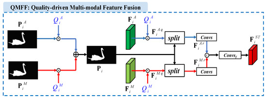
Figure 2.
Detail structure of the quality-driven multi-modal feature fusion (QMFF) module. Here, and refer to the coarse saliency predictions, and denote the quality scores, and is the guidance map. Moreover, and are the level deep features, and refer to the weighted features, and are the refined features, and is the spatiotemporal deep feature.
Firstly, at each level of our network, our video saliency model directly adopts the confidence-guided adaptive gate (CAG) module [17] to estimate the quality scores of spatial features and temporal features. Thus, for the ith level’s deep features, including and , we can obtain the quality scores and , respectively. Meanwhile, by deploying convolutional layers and a sigmoid activation function on and , we can obtain coarse saliency predictions including and , respectively.
Then, the quality scores and coarse saliency predictions are used to generate the guidance map. Concretely, for the ith level encoder network, the coarse saliency predictions and are first weighted by the quality scores and , respectively, and then combined to generate the guidance map , namely
where “·” means scalar multiplication.
Meanwhile, we use the quality scores and to weight the appearance feature and motion features , respectively. This process can be written as
where and refer to the weighted features.
Next, we split the weighted features and into several groups along the channel-wise dimension, and periodically interpolate the guidance map among the split features. Successively, we use convolutional layers to acquire the refined features and , namely
where “” means three 3 × 3 convolutional layers, and “” is the split operation [60]. Here, for the five level features, the split groups are set to 4, 4, 8, 16, and 32, respectively.
Finally, a concatenation operation (“”) and a 1 × 1 convolutional layer (“”) are deployed to fuse two features, yielding the spatiotemporal deep feature . The whole process can be written as
By deploying the quality-driven multi-modal feature fusion (QMFF) module at each level of the encoder network, we can obtain five levels of spatiotemporal deep features .
3.3. Dual-Branched-Based Multi-Level Feature Aggregation
In this section, in order to provide a sufficient aggregation of multi-level spatiotemporal features, we deploy the dual-branched-based multi-level feature aggregation (DMFA) module which contains three steps, including inter-level feature interaction (IFI), dual-branch decoding, and dual-branch fusion (DF). Below, we will provide a detailed description for each part of the DMFA module.
(1) Inter-level Feature Interaction (IFI). The existing encoder–decoder architecture-based networks [61,62] often highlight the main body of salient objects by transferring the encoder features to the decoder layer. However, the low-level spatial details would be disturbed by the continuous accumulation of high-level deep features. Therefore, as shown in Figure 1, we first follow the effort of [8] to deploy the inter-level feature interaction (IFI) unit after each QMFF module, where the IFI unit attempts to fuse the spatiotemporal features from adjacent levels. This promotes the information flow among adjacent level features.
Concretely, we take the ith level for example. We first upsample the higher-level spatiotemporal feature and downsample the lower-level spatiotemporal feature to the same size as the ith level spatiotemporal feature . Then, we concatenate the three-level features along the channel dimension. Lastly, we employ two successive convolutional blocks () to generate the enhanced spatiotemporal feature , of which each convolutional block contains a 3 × 3 convolutional layer, a batch normalization layer (BN), and an ReLU activation function. The whole process can be formulated as
where u refers to the upsampling operation, d denotes the downsampling operation, and means concatenation layer. Here, the convolutional blocks’ channel number is equal to the channel number of the ith level feature .
(2) Dual-branch Decoding. In order to further promote the information exchange and the preserve the spatial details of the salient objects, and inspired by the effort of [24], we also add a parallel decoder branch (i.e., direct concatenation branch) as the supplement to the progressive decoder branch shown in Figure 1, where the direct concatenation branch tries to combine all features from IFI units.
Here, we take the ith level as an example. To be specific, for the traditional progressive decoder branch, we first upsample the higher-level deep feature to the same size as the enhanced spatiotemporal feature . Then, the two features are combined by element-wise summarization and convolutional layers. The whole process can be written as follows:
where denotes the ith level deep decoding feature, and ⊕ is the element wise summation operation. refers to two convolutional blocks, where each block contains a 3 × 3 convolutional layer, a BN layer, and a ReLU activation function. In this way, we can obtain the output of the progressive decoder branch, namely .
Meanwhile, for the direct concatenation branch shown in Figure 1, we first upsample the enhanced spatiotemporal feature to the same spatial size as . Then, we combine them by using a concatenation layer and convolutional layers, namely
where is the fused feature. refers to three convolutional blocks, where each block contains a 3 × 3 convolutional layer, a BN layer, and a ReLU activation function, and the channel number of the three convolutional layers is set to 256, 256, and 32, respectively.
(3) Dual-branch Fusion (DF). In order to aggregate the outputs of two branches, namely and , we design the dual-branch fusion (DF) unit presented in Figure 3. This is considerably different from [24] which simply integrates the saliency predictions of the two outputs via a residual connection.
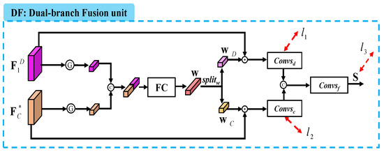
Figure 3.
Illustration of the dual-branch fusion (DF) unit. Here, is the output of the progressive decoder branch, is the fused feature, is the fully connected layer, and is the feature weight, which can be divided into two sub-feature weights and . is the final saliency map, is the split operation, and is the supervision.
Specifically, we first deploy the average pooling layer on each channel of the two features, yielding two vectors which are combined by a concatenation layer and a fully connected layer. This process can be written as follows:
where is the feature weight corresponding to the concatenation of the two features, is the fully connected layer (i.e., 1 × 1 convolutional layer and channel number is 64), and denotes the average pooling layer (i.e., the G in the circle shown in Figure 3).
Then, we split the feature weight into two sub-feature weights and , which are used to weigh and , respectively. Next, we conduct saliency prediction on each weighted feature via a convolutional block including a 1 × 1 convolutional layer (channel=1), an upsampling layer, and a sigmoid activation function. Here, as presented in Figure 3, there are two convolutional blocks, namely and . Finally, the two coarse predictions are further combined to the final saliency map via a convolutional block including a 1 × 1 convolutional layer (channel = 1) and a sigmoid activation function. This process is formulated as follows:
where is the split operation, is the , ⊗ means the dot product, and refer to the two convolutional blocks and , respectively. Moreover, in Figure 4, we present the visualizations for dual-branch fusion. We can see that by deploying the DF unit, the saliency predictions (i.e., , , and ) pay more attention to salient regions, as shown in Figure 4c,e,g.
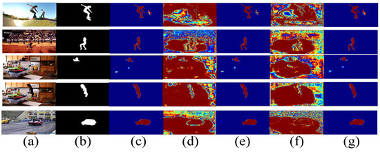
Figure 4.
Visualization of the dual-branch fusion (DF) unit. (a): Input frame, (b): Ground truth, (c): Saliency predictions of , (d): Feature map of , (e): Saliency predictions of , (f): Feature map of , (g): Saliency predictions of .
3.4. Loss Functions
Following the effort [17], we adopt BCE loss [63] and loss to supervise the generation of predicted saliency maps and quality scores. Thus, the first part of loss function can be formulated as
where and are the loss and BCE loss, respectively, and are used to supervise the generation of coarse saliency predictions and quality score in the ith level of the appearance branch. Similarly, and are adopted by the ith level of the motion branch.
Meanwhile, we introduce the hybrid loss [64] including the SSIM loss [65], BCE loss [63], and IoU loss [66] to supervise the saliency prediction in the dual-branch fusion (DF) unit shown in Figure 3, namely
where is the second part of loss function, and employs the hybrid loss. Thus, the total loss of our network can be written as
4. Experimental Results
4.1. Datasets, Implementation Details, and Evaluation Metrics
Here, we evaluate the performance of video saliency models on four benchmark datasets including DAVIS [67], DAVSOD [12], ViSal [32], and SegV2 [68].
We implement our network with PyTorch on a PC, which is equipped with an Intel(R) Xeon(R) E5-2690 2.90 GHz CPU, 32 GB RAM, and an NVIDIA Titan Xp GPU. Our model uses the Adam algorithm [69] to optimize the network, where the initial learning rate, batch size, and maximum epoch number are set to , 4, and 100, respectively. To train our model, we first use the training set of DUTS [70] to train the encoder network including the appearance sub-network and motion sub-network. After that, we adopt the same training set as [17,49,71], namely 30 videos in DAVIS [67] and 90 videos in DAVSOD [12], to train the entire network, where the training time is about 45.5 h. Moreover, we augment the training set by random horizontal flipping and random rotation (0∼180°). Meanwhile, we resize each input image including each frame and its optical flow image to . Moreover, the inference speed (without I/O time), network parameters, and FLOPs of our model are 15 FPS, 145.32 M, and 469.21 G, respectively.
In order to evaluate the model’s performance, we employ the following widely used metrics including precision–recall (PR) curve, F-measure curve, max F-measure (maxF, ) [72], S-measure (S, ) [73], and mean absolute error (MAE).
4.2. Comparison with the State-of-the-Art Methods
We compared our model with 16 state-of-the-art video saliency models on DAVIS, DAVSOD, ViSal, and SegV2 datasets. These video saliency models contain SGSP [42], STBP [36], SFLR [40], SCNN [51], SCOM [37], FGRNE [19], MBNM [46], PDB [11], SSAV [12], MGA [20], PCSA [15], MAGCN [50], STFA [49], GTNet [21], DCFNet [18], and CAG-DDE [17]. Here, the authors do not provide the saliency maps of MAGCN on the DAVSOD and SegV2 datasets, and also do not provide the saliency maps of SCNN on the SegV2 dataset. Therefore, in the quantitative comparison between our model and the state-of-the-art models, we do not show the two models’ results on the DAVSOD and SegV2 datasets.
4.2.1. Quantitative Comparison
We first present the quantitative comparison results including PR curves and F-measure curves in Figure 5. It can be found that our model achieves better performance than other models on the DAVIS and DAVSOD datasets in terms of PR curves and F-measure curves. On the ViSal dataset, our model achieves a comparable performance when compared with some top-level models such as STFA, MGA, and DCFNet. On the SegV2 dataset, our model performs slightly lower than STFA, and presents a comparable performance when compared with some top-level models such as MGA, DCFNet, and CAG-DDE.
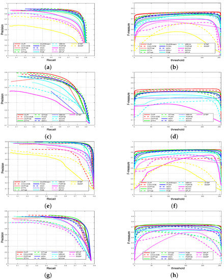
Figure 5.
(Better viewed in color) Quantitative comparison results of different video saliency models: presents (a) PR curves and (b) F-measure curves on DAVIS dataset, presents (c) PR curves and (d) F-measure curves on DAVSOD dataset, presents (e) PR curves and (f) F-measure curves on ViSal dataset, presents (g) PR curves and (h) F-measure curves on SegV2 dataset.
Moreover, we provide MAE, maxF, and S values in Table 1. Compared with the state-of-the-art models, our model still performs best on the DAVIS and DAVSOD datasets. Particularly, compared with the second-best model CAG-DDE on the most challenging dataset DAVSOD, our model improves the performance by 5.06% and 1.31% in terms of maxF and S, respectively, and reduces the MAE by 4.17%. Meanwhile, compared with the top-level models including STFA and DCFNet, our model wins the second place on the ViSal dataset, and achieves the third-best performance on the SegV2 dataset, where the difference is little among the performance of STFA, DCFNet, and our model.

Table 1.
Quantitative comparison results of S, maxF, and MAE on the DAVIS, DAVSOD, ViSal, and SegV2 datasets. Here, “↑” (“↓”) means that the larger (smaller) the better. The top three results in each column are marked in red, green, and blue, respectively.
Here, we should note that though our model and DCFNet employ the same image dataset DUTS [70] to perform the pre-train task, DCFNet is fine-tuned on three video datasets including DAVIS, DAVSOD, and VOS, which endows DCFNet with better generalization ability on the ViSal and SegV2 datasets. Moreover, compared with STFA, we all use DAVIS and DAVSOD datasets to fine-tune the models, but STFA is pre-trained on richer and more diverse image datasets including DUTOMRON [74], HKU-IS [75], and MSRA10K [76], which elevates the generalization ability of the STFA on the ViSal and SegV2 datasets. Generally speaking, according to Figure 5 and Table 1, we can clearly observe the superiority and effectiveness of our model.
4.2.2. Qualitative Comparison
The qualitative comparison results are presented in Figure 6 and Figure 7, where we select three videos from two large-scale benchmark datasets including DAVIS [67] and DAVSOD [12], respectively. Specifically, we make an intuitive comparison between our model and the state-of-the-art models including CAG-DDE [17], DCFNet [18], STFA [49], GTNet [21], MAGCN [50], PCSA [15], MGA [20], SSAV [12], PDB [11], MBNM [46], FGRNE [19], SCOM [37], SCNN [51], SFLR [40], STBP [36], and SGSP [42] in Figure 6. It can be found that our model shown in Figure 6c can precisely locate and segment salient objects in the complex scenes such as the cluttered background (the first row), motion occlusion (the second), and scale variation (the third row). By contrast, the existing video saliency models shown in Figure 6d–s are easily affected by the complex scenes, and they often falsely highlight background regions, pop-out incomplete salient objects, and present coarse spatial details.
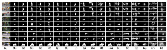
Figure 6.
Qualitative comparison results of different video saliency models on several challenging videos of DAVIS dataset. (a): Video frames, (b): GT, (c): OUR, (d): CAG-DDE, (e): DCFNet, (f): STFA, (g): GTNet, (h): MAGCN, (i): PCSA, (j): MGA, (k): SSAV, (l): PDB, (m): MBNM, (n): FGRNE, (o): SCOM, (p): SCNN, (q): SFLR, (r): STBP, and (s): SGSP.
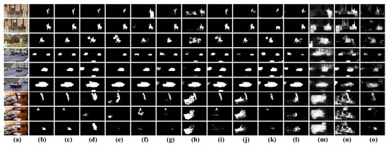
Figure 7.
Qualitative comparison results of different video saliency models on several challenging videos of DAVSOD dataset. (a): Video frames, (b): GT, (c): OUR, (d): CAG-DDE, (e): DCFNet, (f): STFA, (g): GTNet, (h): PCSA, (i): MGA, (j): SSAV, (k): MBNM, (l): FGRNE, (m): SCOM, (n): SCNN, and (o): STBP.
Similarly, in Figure 7, the qualitative comparison is performed between our model and the state-of-the-art models including CAG-DDE [17], DCFNet [18], STFA [49], GTNet [21], MAGCN [50], PCSA [15], MGA [20], SSAV [12], MBNM [46], FGRNE [19], SCOM [37], SCNN [51], and STBP [36]. We can find that our model presented in Figure 7c can accurately discriminate between the human and the horse (the firsts row) and the woman in the kitchen (the third row) from the cluttered background, and effectively pop-out the car from the scene with multiple moving objects (the second row), while other models presented in Figure 7d–o usually falsely highlight background or provide incomplete detection results.
The reason behind this can be attributed to two points. Firstly, the QMFF module of our model fully explores the complementarity of spatial and temporal features, which gives a solid foundation for the multi-modal feature fusion. Secondly, the DMFA module of our model sufficiently aggregates the multi-level spatiotemporal features, which gives more concerns on the main part and local details of salient regions in videos simultaneously. In this way, our model can completely and precisely highlight salient objects in videos.
4.3. Ablation Studies
In order to validate the effectiveness of each component of our model including the quality-driven multi-modal feature fusion (QMFF) module and the dual-branch-based multi-level feature aggregation (DMFA) module, we perform the ablation studies on DAVIS [67] and DAVSOD [12] datasets, where the quantitative comparison results are presented in Table 2 and the qualitative comparison results are provided in Figure 8, Figure 9 and Figure 10.
Table 2.
Quantitative comparison results of different variants of our model in terms of S, maxF, and MAE on the DAVIS and DAVSOD datasets.
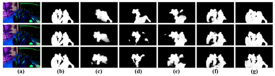
Figure 8.
Qualitative comparisons of four variants of our model. (a): Input frames, (b): GT, (c): w/o QMFF-qf, (d): w/o QMFF-f, (e): w/o QMFF-qp, (f): QMFF-q, and (g): OUR.
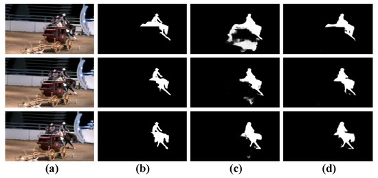
Figure 9.
Qualitative comparisons of the variant of our model. (a): Input frames, (b): GT, (c): w/o IFI, and (d): OUR.
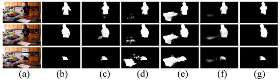
Figure 10.
Qualitative comparisons of four variants of our model. (a): Input frames, (b): GT, (c): w/o db1, (d): w/o db2, (e): w/o DF, (f): w BiFPN, and (g): OUR.
Validation of the QMFF Module. Specifically, firstly, to validate the effectiveness of the quality-driven multi-modal feature fusion (QMFF) module, we present four variants. The first one is “w/o QMFF-qf”, which means our model only adopts a concatenation layer and a 3 × 3 convolutional layer to combine each level’s spatial features and motion features. The second one is “w/o QMFF-f”, which denotes the fact that our model only employs the quality score to re-calibrate (weight) the spatial and temporal features and combines the weighted feature by the concatenation layer and 3 × 3 convolutional layer. The third one is “w/o QMFF-qp”, which denotes that the generation of a guidance map in QMFF module does not employ the quality score. The last one, “w/o QMFF-q”, means that the quality-driven multi-modal feature fusion (QMFF) module does not use the quality score. According to Table 2, we can find that our model performs better than “w/o QMFF-qf”, “w/o QMFF-f”, “w/o QMFF-qp”, and “w/o QMFF-q”. Here, we should note that when compared with the two variants, including “w/o QMFF-qp” and “w/o QMFF-q”, our model achieves a comparable performance in terms of S and MAE on the DAVIS dataset, while our model outperforms the two variants in terms of maxF with a large margin. Moreover, from the qualitative results provided in Figure 8, it can be seen that our model shown in Figure 8g gives an accurate and complete detection for salient objects, while the four variants fail to highlight the people in the ballroom shown in Figure 8c–f. Particularly, the performance of the variant “w/o QMFF-f” shown in Figure 8d is greatly degraded. Thus, according to the aforementioned descriptions, we can firmly prove the effectiveness and rationality of the quality-driven multi-modal feature fusion (QMFF) module.
Validation of the QMFA module. Then, in order to demonstrate the effectiveness of the inter-level feature interaction (IFI) unit, we devise a variant “w/o IFI”, i.e., our model without IFI units. From Table 2, we can find that our model outperforms “w/o IFI” on both datasets. Meanwhile, through the qualitative presentation shown in Figure 9, it can be seen that “w/o IFI” falsely highlights some background regions, while under the employment of IFI units, our model gives accurate detection results. This can prove the rationality of the utilization of the IFI units in our model.
Next, in order to prove the effectiveness of the dual-branch-based multi-level feature aggregation (QMFA) module, we design three variants, namely our model without the progressive decoder branch (“w/o db1”), our model without the parallel decoder branch (“w/o db2”), and our model without the dual-branch fusion (DF) unit (“w/o DF”). After removing one branch, the output of each branch is processed by a 1 × 1 convolutional layer (channel = 1) and a sigmoid activation function, yielding the final saliency map. For “w/o DF”, this means that our model employs a concatenation layer, a 1 × 1 convolutional layer, and a sigmoid activation function to replace the DF unit. Moreover, we also employ the bi-directional feature pyramid structure [77] to replace the QMFA module, namely “w BiFPN”. According to Table 2, we can find that our model performs better than “w/o db2”, “w/o DF”, and “w BiFPN” on both datasets. When compared with “w/o db1”, our model exhibits a superior performance on the DAVSOD dataset, and achieves a comparable performance on the DAVIS dataset. Meanwhile, in the qualitative comparison results shown in Figure 10, it can be seen that “w/o db1”, “w BiFPN”, and “w/o DF” highlight the background regions mistakenly, and that “w/o db2” presents incomplete detection results. By contrast, the results of our model shown in Figure 10g are the closest one to the ground truth. Therefore, through the above quantitative and qualitative comparison results, we can prove the effectiveness and rationality of the dual-branch-based multi-level feature aggregation (DMFA) module.
Lastly, to evaluate the effect of the loss weights in Equation (12), we design a variant “w lw”, which means that the loss function in Equation (12) adopt weights (i.e., ). The results are presented in Table 2 and Figure 11. From the quantitative results presented in Table 2, we can see that our model performs better than “w lw”. For the qualitative results shown in Figure 11, “w lw” falsely highlights background regions. Therefore, we can prove the effectiveness of the loss function in Equation (12) where the weights of and are all set to 1.
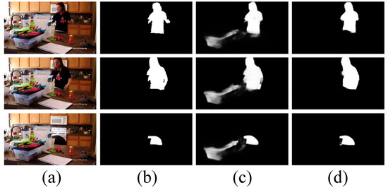
Figure 11.
Qualitative comparisons of a variant of our model. (a): Input frames, (b): GT, (c): w lw, and (d): OUR.
4.4. Failure Cases and Analysis
From the above descriptions, our proposed model can effectively pop-out salient objects in videos. However, our method is still unable to present promising results when addressing some complex scenes, as shown in Figure 12. For example, in the first example (i.e., the first and second columns), a dog with black fur is standing by the river, where goldfish are in the river and a dog with white fur all over it is also standing by the river. In Figure 12c, our model falsely highlights the white dog’s head and a goldfish. It can be seen that the inference results cannot accurately detect salient objects when the scene comprises complex background. For the second example (i.e., the third and fourth columns), a man is riding a horse. From Figure 12c, we can see that our model mistakenly highlights the fence barrier. Similarly, in the third example (i.e., the fifth and sixth columns), a man is surfing. Our model still falsely highlights the background regions. Moreover, we also find that the annotation is worthy of discussion. For example, in the first example (i.e., the first column), both dogs are attractive to human eyes. In the second example, our human eyes will be also the first to notice the fence barrier. In the third example, the spindrift around the man (i.e., the fifth column) and the people after the surfer (i.e., the sixth column) are also the regions of interest for our human eyes. All the attractive regions should be annotated as salient objects. In order to address the two issues above, on one hand, we should pay more attention to the design of video saliency models, where the encoder should provide more effective features for characterization of salient objects. On the other hand, we will attempt to find and correct the ambiguity-labeling samples.
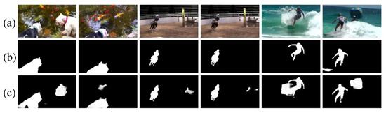
Figure 12.
Some failure examples of our model. (a): Input frames, (b): Ground truth, and (c): Saliency maps generated by our model.
5. Conclusions
This paper proposes a quality-driven dual-branch feature integration network to detect salient objects in videos, where the key components are the quality-driven multi-modal feature fusion (QMFF) module and the dual-branch-based multi-level feature aggregation (DMFA) module. Firstly, in the QMFF module, we fully explore the complementarity of spatial and temporal features, and thereby we can provide an appropriate fusion of multi-modal features. Particularly, the quality scores are introduced to re-calibrate the two modal features and integrate the coarse saliency predictions into a guidance map which further promotes the features to pay more attention to salient regions. Secondly, we deploy an effective aggregation scheme, namely the DMFA module, to sufficiently fuse multi-level spatiotemporal features. In the DMFA module, we design the dual-branch fusion (DF) unit to effectively fuse the outputs of dual branch decoders including the progressive decoder branch and the direction concatenation branch. Comprehensive experiments are performed on four public video datasets, where the quantitative and qualitative comparison results firmly prove the effectiveness of the proposed video saliency model.
Author Contributions
Methodology, X.Z. and H.G.; Software, H.G. and L.Y.; Validation, D.Y.; Writing—original draft, X.Z.; Writing—review & editing, L.Y.; Supervision, X.Z.; Project administration, H.G.; Funding acquisition, J.Z. All authors have read and agreed to the published version of the manuscript.
Funding
This work was supported in part by the National Natural Science Foundation of China under Grants 62271180 and 61901145, in part by the Fundamental Research Funds for the Provincial Universities of Zhejiang under Grants GK229909299001-009, in part by the Zhejiang Province Nature Science Foundation of China under Grant LZ22F020003, and in part by the Hangzhou Dianzi University (HDU) and the China Electronics Corporation DATA (CECDATA) Joint Research Center of Big Data Technologies under Grant KYH063120009.
Data Availability Statement
Not applicable.
Conflicts of Interest
The authors declare no conflict of interest.
References
- Tung, F.; Zelek, J.S.; Clausi, D.A. Goal-based trajectory analysis for unusual behaviour detection in intelligent surveillance. Image Vis. Comput. 2011, 29, 230–240. [Google Scholar] [CrossRef]
- Verlekar, T.T.; Soares, L.D.; Correia, P.L. Gait recognition in the wild using shadow silhouettes. Image Vis. Comput. 2018, 76, 1–13. [Google Scholar] [CrossRef]
- Li, Z.; Qin, S.; Itti, L. Visual attention guided bit allocation in video compression. Image Vis. Comput. 2011, 29, 1–14. [Google Scholar] [CrossRef]
- Zheng, B.; Chen, Y.; Tian, X.; Zhou, F.; Liu, X. Implicit dual-domain convolutional network for robust color image compression artifact reduction. IEEE Trans. Circuits Syst. Video Technol. 2020, 30, 3982–3994. [Google Scholar] [CrossRef]
- Hendry; Chen, R.C. Automatic License Plate Recognition via sliding-window darknet-YOLO deep learning. Image Vis. Comput. 2019, 87, 47–56. [Google Scholar] [CrossRef]
- Zhou, X.; Li, G.; Gong, C.; Liu, Z.; Zhang, J. Attention-guided RGBD saliency detection using appearance information. Image Vis. Comput. 2020, 95, 103888. [Google Scholar] [CrossRef]
- Wu, Z.; Li, S.; Chen, C.; Hao, A.; Qin, H. A deeper look at image salient object detection: Bi-stream network with a small training dataset. IEEE Trans. Multimed. 2020, 24, 73–86. [Google Scholar] [CrossRef]
- Pang, Y.; Zhao, X.; Zhang, L.; Lu, H. Multi-scale interactive network for salient object detection. In Proceedings of the IEEE Conference on Computer Vision and Pattern Recognition (CVPR), Seattle, WA, USA, 13–19 June 2020; pp. 9413–9422. [Google Scholar]
- Wang, W.; Shen, J.; Shao, L. Video salient object detection via fully convolutional networks. IEEE Trans. Image Process. 2017, 27, 38–49. [Google Scholar] [CrossRef]
- Sun, M.; Zhou, Z.; Hu, Q.; Wang, Z.; Jiang, J. SG-FCN: A motion and memory-based deep learning model for video saliency detection. IEEE Trans. Cybern. 2018, 49, 2900–2911. [Google Scholar] [CrossRef]
- Song, H.; Wang, W.; Zhao, S.; Shen, J.; Lam, K.M. Pyramid dilated deeper convlstm for video salient object detection. In Computer Vision—ECCV 2018, Proceedings of the 15th European Conference, Munich, Germany, 8–14 September 2018; Springer Nature: Cham, Switzerland, 2018; pp. 715–731. [Google Scholar]
- Fan, D.P.; Wang, W.; Cheng, M.M.; Shen, J. Shifting more attention to video salient object detection. In Proceedings of the IEEE Conference on Computer Vision and Pattern Recognition (CVPR), Long Beach, CA, USA, 15–20 June 2019; pp. 8554–8564. [Google Scholar]
- Le, T.N.; Sugimoto, A. Deeply Supervised 3D Recurrent FCN for Salient Object Detection in Videos. In Proceedings of the 28th British Machine Vision Conference (BMVC), London, UK, 4–9 September 2017; Volume 1, pp. 1–13. [Google Scholar]
- Dong, S.; Gao, Z.; Pirbhulal, S.; Bian, G.B.; Zhang, H.; Wu, W.; Li, S. IoT-based 3D convolution for video salient object detection. Neural Comput. Appl. 2020, 32, 735–746. [Google Scholar] [CrossRef]
- Gu, Y.; Wang, L.; Wang, Z.; Liu, Y.; Cheng, M.M.; Lu, S.P. Pyramid constrained self-attention network for fast video salient object detection. Proc. AAAI Conf. Artif. Intell. 2020, 34, 10869–10876. [Google Scholar] [CrossRef]
- Bi, H.; Yang, L.; Zhu, H.; Lu, D.; Jiang, J. STEG-Net: Spatio-Temporal Edge Guidance Network for Video Salient Object Detection. IEEE Trans. Cogn. Dev. Syst. 2021, 14, 902–915. [Google Scholar] [CrossRef]
- Chen, P.; Lai, J.; Wang, G.; Zhou, H. Confidence-Guided Adaptive Gate and Dual Differential Enhancement for Video Salient Object Detection. In Proceedings of the 2021 IEEE International Conference on Multimedia and Expo (ICME), Shenzhen, China, 5–9 July 2021; pp. 1–6. [Google Scholar]
- Zhang, M.; Liu, J.; Wang, Y.; Piao, Y.; Yao, S.; Ji, W.; Li, J.; Lu, H.; Luo, Z. Dynamic context-sensitive filtering network for video salient object detection. In Proceedings of the IEEE International Conference on Computer Vision (ICCV), Montreal, QC, Canada, 10–17 October 2021; pp. 1553–1563. [Google Scholar]
- Li, G.; Xie, Y.; Wei, T.; Wang, K.; Lin, L. Flow guided recurrent neural encoder for video salient object detection. In Proceedings of the IEEE Conference on Computer Vision and Pattern Recognition (CVPR), Salt Lake City, UT, USA, 18–23 June 2018; pp. 3243–3252. [Google Scholar]
- Li, H.; Chen, G.; Li, G.; Yu, Y. Motion guided attention for video salient object detection. In Proceedings of the IEEE Conference on Computer Vision and Pattern Recognition (CVPR), Seoul, Republic of Korea, 27 October–2 November 2019; pp. 7274–7283. [Google Scholar]
- Jiao, Y.; Wang, X.; Chou, Y.C.; Yang, S.; Ji, G.P.; Zhu, R.; Gao, G. Guidance and Teaching Network for Video Salient Object Detection. In Proceedings of the 2021 IEEE International Conference on Image Processing (ICIP), Anchorage, AK, USA, 19–22 September 2021; pp. 2199–2203. [Google Scholar]
- Chen, C.; Song, J.; Peng, C.; Wang, G.; Fang, Y. A Novel Video Salient Object Detection Method via Semisupervised Motion Quality Perception. IEEE Trans. Circuits Syst. Video Technol. 2021, 32, 2732–2745. [Google Scholar] [CrossRef]
- Chen, C.; Wei, J.; Peng, C.; Qin, H. Depth-quality-aware salient object detection. IEEE Trans. Image Process. 2021, 30, 2350–2363. [Google Scholar] [CrossRef]
- Zhao, X.; Pang, Y.; Zhang, L.; Lu, H.; Zhang, L. Suppress and balance: A simple gated network for salient object detection. In Computer Vision—ECCV 2020, Proceedings of the 16th European Conference, Glasgow, UK, 23–28 August 2020; Springer: Cham, Switzerland, 2020; pp. 35–51. [Google Scholar]
- Ma, T.; Yang, M.; Rong, H.; Qian, Y.; Tian, Y.; Al-Nabhan, N. Dual-path CNN with Max Gated block for text-based person re-identification. Image Vis. Comput. 2021, 111, 104168. [Google Scholar] [CrossRef]
- Khorramshahi, P.; Kumar, A.; Peri, N.; Rambhatla, S.S.; Chen, J.C.; Chellappa, R. A dual-path model with adaptive attention for vehicle re-identification. In Proceedings of the IEEE/CVF International Conference on Computer Vision, Seoul, Republic of Korea, 27 October–2 November 2019; pp. 6132–6141. [Google Scholar]
- Zheng, Z.; Zheng, L.; Garrett, M.; Yang, Y.; Xu, M.; Shen, Y.D. Dual-path convolutional image-text embeddings with instance loss. ACM Trans. Multimed. Comput. Commun. Appl. 2020, 16, 1–23. [Google Scholar] [CrossRef]
- Zhang, P.; Wang, D.; Lu, H.; Wang, H.; Ruan, X. Amulet: Aggregating multi-level convolutional features for salient object detection. In Proceedings of the IEEE International Conference on Computer Vision (ICCV), Venice, Italy, 22–29 October 2017; pp. 202–211. [Google Scholar]
- Liu, Z.; Wang, Y.; Tu, Z.; Xiao, Y.; Tang, B. TriTransNet: RGB-D salient object detection with a triplet transformer embedding network. In Proceedings of the 29th ACM International Conference on Multimedia, Virtual, 20–24 October 2021; pp. 4481–4490. [Google Scholar]
- Liu, Z.; Tan, Y.; He, Q.; Xiao, Y. SwinNet: Swin Transformer drives edge-aware RGB-D and RGB-T salient object detection. arXiv 2022, arXiv:2204.05585. [Google Scholar] [CrossRef]
- Liu, H.; Zhang, J.; Yang, K.; Hu, X.; Stiefelhagen, R. CMX: Cross-Modal Fusion for RGB-X Semantic Segmentation with Transformers. arXiv 2022, arXiv:2203.04838. [Google Scholar]
- Wang, W.; Shen, J.; Shao, L. Consistent video saliency using local gradient flow optimization and global refinement. IEEE Trans. Image Process. 2015, 24, 4185–4196. [Google Scholar] [CrossRef]
- Wang, W.; Shen, J.; Porikli, F. Saliency-aware geodesic video object segmentation. In Proceedings of the IEEE Conference on Computer Vision and Pattern Recognition (CVPR), Boston, MA, USA, 7–12 June 2015; pp. 3395–3402. [Google Scholar]
- Zhou, X.; Liu, Z.; Li, K.; Sun, G. Video saliency detection via bagging-based prediction and spatiotemporal propagation. J. Vis. Commun. Image Represent. 2018, 51, 131–143. [Google Scholar] [CrossRef]
- Fang, Y.; Wang, Z.; Lin, W.; Fang, Z. Video saliency incorporating spatiotemporal cues and uncertainty weighting. IEEE Trans. Image Process. 2014, 23, 3910–3921. [Google Scholar] [CrossRef] [PubMed]
- Xi, T.; Zhao, W.; Wang, H.; Lin, W. Salient object detection with spatiotemporal background priors for video. IEEE Trans. Image Process. 2016, 26, 3425–3436. [Google Scholar] [CrossRef] [PubMed]
- Chen, Y.; Zou, W.; Tang, Y.; Li, X.; Xu, C.; Komodakis, N. SCOM: Spatiotemporal constrained optimization for salient object detection. IEEE Trans. Image Process. 2018, 27, 3345–3357. [Google Scholar] [CrossRef] [PubMed]
- Kim, H.; Kim, Y.; Sim, J.Y.; Kim, C.S. Spatiotemporal saliency detection for video sequences based on random walk with restart. IEEE Trans. Image Process. 2015, 24, 2552–2564. [Google Scholar] [CrossRef]
- Li, Y.; Tan, Y.; Yu, J.G.; Qi, S.; Tian, J. Kernel regression in mixed feature spaces for spatio-temporal saliency detection. Comput. Vis. Image Underst. 2015, 135, 126–140. [Google Scholar] [CrossRef]
- Chen, C.; Li, S.; Wang, Y.; Qin, H.; Hao, A. Video saliency detection via spatial-temporal fusion and low-rank coherency diffusion. IEEE Trans. Image Process. 2017, 26, 3156–3170. [Google Scholar] [CrossRef]
- Chen, C.; Li, S.; Qin, H.; Pan, Z.; Yang, G. Bilevel feature learning for video saliency detection. IEEE Trans. Multimed. 2018, 20, 3324–3336. [Google Scholar] [CrossRef]
- Liu, Z.; Li, J.; Ye, L.; Sun, G.; Shen, L. Saliency detection for unconstrained videos using superpixel-level graph and spatiotemporal propagation. IEEE Trans. Circuits Syst. Video Technol. 2016, 27, 2527–2542. [Google Scholar] [CrossRef]
- Zhou, X.; Liu, Z.; Gong, C.; Liu, W. Improving video saliency detection via localized estimation and spatiotemporal refinement. IEEE Trans. Multimed. 2018, 20, 2993–3007. [Google Scholar] [CrossRef]
- Guo, F.; Wang, W.; Shen, J.; Shao, L.; Yang, J.; Tao, D.; Tang, Y.Y. Video saliency detection using object proposals. IEEE Trans. Cybern. 2017, 48, 3159–3170. [Google Scholar] [CrossRef]
- Guo, F.; Wang, W.; Shen, Z.; Shen, J.; Shao, L.; Tao, D. Motion-aware rapid video saliency detection. IEEE Trans. Circuits Syst. Video Technol. 2019, 30, 4887–4898. [Google Scholar] [CrossRef]
- Li, S.; Seybold, B.; Vorobyov, A.; Lei, X.; Kuo, C.C.J. Unsupervised video object segmentation with motion-based bilateral networks. In Computer Vision—ECCV 2018, Proceedings of the 15th European Conference, Munich, Germany, 8–14 September 2018; Springer: Cham, Switzerland, 2018; pp. 207–223. [Google Scholar]
- Wen, H.; Zhou, X.; Sun, Y.; Zhang, J.; Yan, C. Deep fusion based video saliency detection. J. Vis. Commun. Image Represent. 2019, 62, 279–285. [Google Scholar] [CrossRef]
- Li, Y.; Li, S.; Chen, C.; Hao, A.; Qin, H. A plug-and-play scheme to adapt image saliency deep model for video data. IEEE Trans. Circuits Syst. Video Technol. 2020, 31, 2315–2327. [Google Scholar] [CrossRef]
- Chen, C.; Wang, G.; Peng, C.; Fang, Y.; Zhang, D.; Qin, H. Exploring rich and efficient spatial temporal interactions for real-time video salient object detection. IEEE Trans. Image Process. 2021, 30, 3995–4007. [Google Scholar] [CrossRef]
- Xu, M.; Fu, P.; Liu, B.; Li, J. Multi-Stream Attention-Aware Graph Convolution Network for Video Salient Object Detection. IEEE Trans. Image Process. 2021, 30, 4183–4197. [Google Scholar] [CrossRef]
- Tang, Y.; Zou, W.; Jin, Z.; Chen, Y.; Hua, Y.; Li, X. Weakly supervised salient object detection with spatiotemporal cascade neural networks. IEEE Trans. Circuits Syst. Video Technol. 2018, 29, 1973–1984. [Google Scholar] [CrossRef]
- Yan, P.; Li, G.; Xie, Y.; Li, Z.; Wang, C.; Chen, T.; Lin, L. Semi-supervised video salient object detection using pseudo-labels. In Proceedings of the IEEE International Conference on Computer Vision (ICCV), Seoul, Republic of Korea, 27 October–2 November 2019; pp. 7284–7293. [Google Scholar]
- Le, T.N.; Sugimoto, A. Video salient object detection using spatiotemporal deep features. IEEE Trans. Image Process. 2018, 27, 5002–5015. [Google Scholar] [CrossRef]
- Fang, Y.; Ding, G.; Li, J.; Fang, Z. Deep3DSaliency: Deep stereoscopic video saliency detection model by 3D convolutional networks. IEEE Trans. Image Process. 2018, 28, 2305–2318. [Google Scholar] [CrossRef]
- Zhou, X.; Shen, K.; Liu, Z.; Gong, C.; Zhang, J.; Yan, C. Edge-aware multiscale feature integration network for salient object detection in optical remote sensing images. IEEE Trans. Geosci. Remote Sens. 2021, 60, 5605315. [Google Scholar] [CrossRef]
- Zhou, X.; Fang, H.; Liu, Z.; Zheng, B.; Sun, Y.; Zhang, J.; Yan, C. Dense Attention-guided Cascaded Network for Salient Object Detection of Strip Steel Surface Defects. IEEE Trans. Instrum. Meas. 2021, 71, 5004914. [Google Scholar] [CrossRef]
- Zhou, X.; Wen, H.; Shi, R.; Yin, H.; Zhang, J.; Yan, C. FANet: Feature aggregation network for RGBD saliency detection. Signal Process. Image Commun. 2022, 102, 116591. [Google Scholar] [CrossRef]
- Teed, Z.; Deng, J. Raft: Recurrent all-pairs field transforms for optical flow. In Computer Vision—ECCV 2020, Proceedings of the 16th European Conference, Glasgow, UK, 23–28 August 2020; Springer: Cham, Switzerlad, 2020; pp. 402–419. [Google Scholar]
- He, K.; Zhang, X.; Ren, S.; Sun, J. Deep residual learning for image recognition. In Proceedings of the IEEE Conference on Computer Vision and Pattern Recognition (CVPR), Las Vegas, NV, USA, 27–30 June 2016; pp. 770–778. [Google Scholar]
- Fan, D.P.; Ji, G.P.; Cheng, M.M.; Shao, L. Concealed object detection. IEEE Trans. Pattern Anal. Mach. Intell. 2021, 44, 6024–6042. [Google Scholar] [CrossRef] [PubMed]
- Long, J.; Shelhamer, E.; Darrell, T. Fully convolutional networks for semantic segmentation. In Proceedings of the IEEE Conference on Computer Vision and Pattern Recognition (CVPR), Boston, MA, USA, 7–12 June 2015; pp. 3431–3440. [Google Scholar]
- Zhang, L.; Dai, J.; Lu, H.; He, Y.; Wang, G. A bi-directional message passing model for salient object detection. In Proceedings of the IEEE Conference on Computer Vision and Pattern Recognition (CVPR), Salt Lake City, UT, USA, 18–23 June 2018; pp. 1741–1750. [Google Scholar]
- De Boer, P.T.; Kroese, D.P.; Mannor, S.; Rubinstein, R.Y. A tutorial on the cross-entropy method. Ann. Oper. Res. 2005, 134, 19–67. [Google Scholar] [CrossRef]
- Qin, X.; Zhang, Z.; Huang, C.; Gao, C.; Dehghan, M.; Jagersand, M. Basnet: Boundary-aware salient object detection. In Proceedings of the IEEE Conference on Computer Vision and Pattern Recognition (CVPR), Long Beach, CA, USA, 15–20 June 2019; pp. 7479–7489. [Google Scholar]
- Wang, Z.; Simoncelli, E.P.; Bovik, A.C. Multiscale structural similarity for image quality assessment. In Proceedings of the 37th Asilomar Conference on Signals, Systems & Computers, Pacific Grove, CA, USA, 9–12 November 2003; Volume 2, pp. 1398–1402. [Google Scholar]
- Máttyus, G.; Luo, W.; Urtasun, R. Deeproadmapper: Extracting road topology from aerial images. In Proceedings of the International Conference on Computer Vision (ICCV), Venice, Italy, 22–29 October 2017; pp. 3438–3446. [Google Scholar]
- Perazzi, F.; Pont-Tuset, J.; McWilliams, B.; Van Gool, L.; Gross, M.; Sorkine-Hornung, A. A benchmark dataset and evaluation methodology for video object segmentation. In Proceedings of the IEEE Conference on Computer Vision and Pattern Recognition (CVPR), Las Vegas, NV, USA, 27–30 June 2016; pp. 724–732. [Google Scholar]
- Li, F.; Kim, T.; Humayun, A.; Tsai, D.; Rehg, J.M. Video segmentation by tracking many figure-ground segments. In Proceedings of the IEEE Conference on Computer Vision and Pattern Recognition (CVPR), Sydney, NSW, Australia, 1–8 December 2013; pp. 2192–2199. [Google Scholar]
- Da, K. A method for stochastic optimization. arXiv 2014, arXiv:1412.6980. [Google Scholar]
- Wang, L.; Lu, H.; Wang, Y.; Feng, M.; Wang, D.; Yin, B.; Ruan, X. Learning to detect salient objects with image-level supervision. In Proceedings of the IEEE Conference on Computer Vision and Pattern Recognition (CVPR), Honolulu, HI, USA, 21–26 July 2017; pp. 136–145. [Google Scholar]
- Wang, B.; Liu, W.; Han, G.; He, S. Learning long-term structural dependencies for video salient object detection. IEEE Trans. Image Process. 2020, 29, 9017–9031. [Google Scholar] [CrossRef]
- Achanta, R.; Hemami, S.; Estrada, F.; Susstrunk, S. Frequency-tuned salient region detection. In Proceedings of the IEEE Conference on Computer Vision and Pattern Recognition (CVPR), Miami, FL, USA, 20–25 June 2009; pp. 1597–1604. [Google Scholar]
- Fan, D.P.; Cheng, M.M.; Liu, Y.; Li, T.; Borji, A. Structure-measure: A new way to evaluate foreground maps. In Proceedings of the International Conference on Computer Vision (ICCV), Venice, Italy, 22–29 October 2017; pp. 4548–4557. [Google Scholar]
- Yang, C.; Zhang, L.; Lu, H.; Ruan, X.; Yang, M.H. Saliency detection via graph-based manifold ranking. In Proceedings of the IEEE Conference on Computer Vision and Pattern Recognition (CVPR), Portland, OR, USA, 23–28 June 2013; pp. 3166–3173. [Google Scholar]
- Li, G.; Yu, Y. Visual saliency detection based on multiscale deep CNN features. IEEE Trans. Image Process. 2016, 25, 5012–5024. [Google Scholar] [CrossRef]
- Cheng, M.M.; Mitra, N.J.; Huang, X.; Torr, P.H.; Hu, S.M. Global contrast based salient region detection. IEEE Trans. Pattern Anal. Mach. Intell. 2014, 37, 569–582. [Google Scholar] [CrossRef]
- Tan, M.; Pang, R.; Le, Q.V. Efficientdet: Scalable and efficient object detection. In Proceedings of the IEEE/CVF Conference on Computer Vision and Pattern Recognition, Seattle, WA, USA, 13–19 June 2020; pp. 10781–10790. [Google Scholar]


Disclaimer/Publisher’s Note: The statements, opinions and data contained in all publications are solely those of the individual author(s) and contributor(s) and not of MDPI and/or the editor(s). MDPI and/or the editor(s) disclaim responsibility for any injury to people or property resulting from any ideas, methods, instructions or products referred to in the content. |
© 2023 by the authors. Licensee MDPI, Basel, Switzerland. This article is an open access article distributed under the terms and conditions of the Creative Commons Attribution (CC BY) license (https://creativecommons.org/licenses/by/4.0/).