Article

Model-Based Coordinated Trajectory Tracking Control of Skid-Steer Mobile Robot with Timing-Belt Servo System

1
School of Mechatronics Engineering, Harbin Institute of Technology, Harbin 150001, China
2
Division of Information Science and Technology, Tsinghua Shenzhen International Graduate School, Shenzhen 518055, China
3
Research and Development Centre for Intelligent Control and Advanced Manufacturing, Research Institute of Tsinghua University, Shenzhen 518054, China
*
Authors to whom correspondence should be addressed.
Electronics 2023, 12(3), 699; https://doi.org/10.3390/electronics12030699
Submission received: 26 November 2022 / Revised: 28 January 2023 / Accepted: 29 January 2023 / Published: 31 January 2023
(This article belongs to the Special Issue Design, Dynamics and Control of Robots)

Abstract

:
Four-wheel, independently driven skid-steer mobile robots have been widely used in some fields, such as indoor product shipping and outdoor inspection and exploration. Traditional skid-steer mobile robot controllers often use a kinematics controller to obtain the desired speed of each wheel, complete speed closed-loop control of each wheel and achieve the robot’s trajectory tracking control. However, the controller based on kinematics may lead to robot chattering and wheel spin from being directly driven by the motor on uneven grounds. To solve these problems, we developed a four-wheel, independently driven skid-steer mobile robot with a damping module for the timing-belt servo system and proposed a model-based coordinated trajectory tracking control method with the timing-belt servo system. First, the kinematics and dynamics of the mobile robot are established, including the chassis kinematics and dynamics, as well as the dynamics of the timing-belt servo system. Secondly, the hierarchical control law is designed, which has adaptive robust control of the upper-level robot chassis, middle-level control allocation approach, and adaptive robust control of the bottom-level timing-belt servo system. Finally, the proposed method is verified by the robot’s trajectory tracking control comparison simulation experiments and has a better control performance.

1. Introduction

In recent years, mobile robots have been increasingly used in industrial automation, agriculture, and service industries, as well as defense industries, such as inspection, exploration, and rescue after a disaster [1,2,3,4]. The skid-steer-type mobile robots, due to their strong flexibility, high pass ability, and good adaptability, are often used in the above tasks. Traditional four-wheel, independently driven skid-steer mobile robots are often driven directly by motors [3], i.e., each wheel is equipped with a directly driven motor, which has the advantage of a simple drive system. Compared with the direct drive method, the timing-belt servo system has the advantages of being lightweight, vibration absorption, and high torque [5]. Based on these characteristics, timing-belt servo systems have been widely used in automotive, textile, agricultural machines, and robotic motion [5,6,7,8,9]. In addition, the four-wheel, independent drive makes the robot have redundant drive characteristics, which can make the robot have higher load capacity, stronger motion capability, and good fault tolerance characteristics. Currently, major universities and research institutes have performed a lot of studies on the trajectory tracking control of the mobile robot [10,11,12,13], but they are focused on the two-wheel drive and car-like model mobile robot control. Among them, there are relatively few studies [3] on the trajectory tracking control of the four-wheel, independently driven skid-steer mobile robots.
The trajectory tracking control of the skid-steer-type mobile robot has two types; kinematics and dynamics controllers. The controller based on the robot kinematics model can directly plan the output speed command of each driven wheel, which does not consider the slipping phenomenon of the robot chassis [14,15]. In addition, the skid-steer mobile robots, due to the lack of steering systems, achieve steering by the different wheel speeds on both sides of the robot, which is also prone to producing a slipping phenomenon from the kinematics controller [16]. In order to improve the control performance of the skid-steer-type mobile robot, considering the slipping phenomenon, the control strategy of the skid-steer mobile robot based on the dynamics model has been proposed [2,17,18]. Compared with the kinematics controller, the dynamics controller can directly plan the driving force command of each wheel.
The control strategy of the skid-steer-type mobile robot based on the dynamics model brings model uncertainty and nonlinear problems [19], which also brings a lot of challenges to mobile robot motion planning control. Thus, there have been a lot of studies on the model uncertainty and nonlinear problems of mobile robots. In [2,10], an adaptive control method to consider the slipping effects and a robust control method in the condition of mobile robot slipping are proposed, which solves the model uncertainty problem of the skid-steer mobile robot. In [3], taking into account parameters and model uncertainty, a skid-steer mobile robot adaptive robust control method was proposed. The trajectory tracking of the skid-steer mobile robot adopted the adaptive robust control law based on the dynamics model has good performance.
Moreover, the four-wheel, independently driven skid-steer mobile robots also need to consider the issue of their redundant drive [3]. Although the mobile robots with redundant drive have stronger power and better safety, which do not break down due to a certain driver wheel failure, they also bring a lot of challenges for the coordination control due to the four wheels being independently driven. For electric ground vehicles, some control allocation methods have been proposed [20,21], where the controller is developed from the direct allocation of driving force through energy compensation. In [22], a global-local control allocation method is proposed, where the global controller generates a reference driving force, and the local controller controls the direct force information from the global controller. In [3], a torque allocation control with feedback compensation to limit the wheel velocity is proposed, which provides a simplified control solution for the redundant drive of the four-wheel mobile robot. Through these control allocation methods, the corresponding control objects have achieved good control effects. Therefore, in order to make the skid-steer-type mobile robots have better control performance, we proposed a driving force allocation method to solve the problem of the skid-steer mobile robot redundantly driven based on the dynamics model.
In this paper, each driving mechanism of the skid-steer mobile robot has a modular timing-belt servo system, which is equipped with a damping buffer device and can ensure full contact between the wheels and the ground to improve the slipping problem of the mobile robot. In addition, in order to solve the slipping problem caused by the contact of the wheels and ground, it is important to establish a driving wheel dynamics model. In [2], the modeling of the wheel-ground is proposed for the skid-steer mobile robots. Some research works also developed the controller with consideration of the slipping phenomenon [10,21]. However, these studies [23,24,25,26,27,28] have not been further discussed in the driving wheel dynamics model and wheel-ground interactions. Moreover, lots of model-based control laws and adaptive robust controllers [8,14] have been developed. Furthermore, considering the advantages of good shock absorption and anti-buffer of the timing-belt servo system, we propose an adaptive robust control method of the timing-belt servo system based on the dynamics model to solve the driving wheel slipping problems.
The new contribution of this paper is that we develop a four-wheel, independently driven, skid-steer mobile robot with a timing-belt servo system that has a damping module, as shown in Figure 1, and propose a coordinated control method based on dynamics models. In addition, different from the robots with a direct motor drive, the developed robot, which has a timing-belt servo system with a damping module, can increase drive torque and improve the contact between the wheels and the ground. Furthermore, the proposed controller based on dynamics models adopted a hierarchical control architecture to solve the problems about the parameters and model uncertainties, being redundantly driven and slipping. Moreover, the stability of the proposed controller is guaranteed by theoretical proof. Finally, the proposed controller has a good trajectory tracking control performance and a smaller tracking error from the simulation experiment compared with the traditional kinematics and dynamics controllers. Thus, compared to traditional kinematics and dynamic model controllers, the proposed controller of this paper is useful for the development of controllers of four-wheel, independently driven skid-steer mobile robots.
The rest of this paper is arranged as follows. In the second part, we establish the models, including the kinematics and dynamics of the chassis and the dynamics of the timing-belt servo system, for the four-wheel, independently driven skid-steer mobile robot with timing-belt servo system. In the third part, the controller, including a hierarchical control architecture for the trajectory tracking control of the mobile robot, is proposed. The mobile robot test platform and the comparison of the results are presented in the fourth part. Finally, the conclusion of this paper is placed in the fifth part.

2. System Modeling

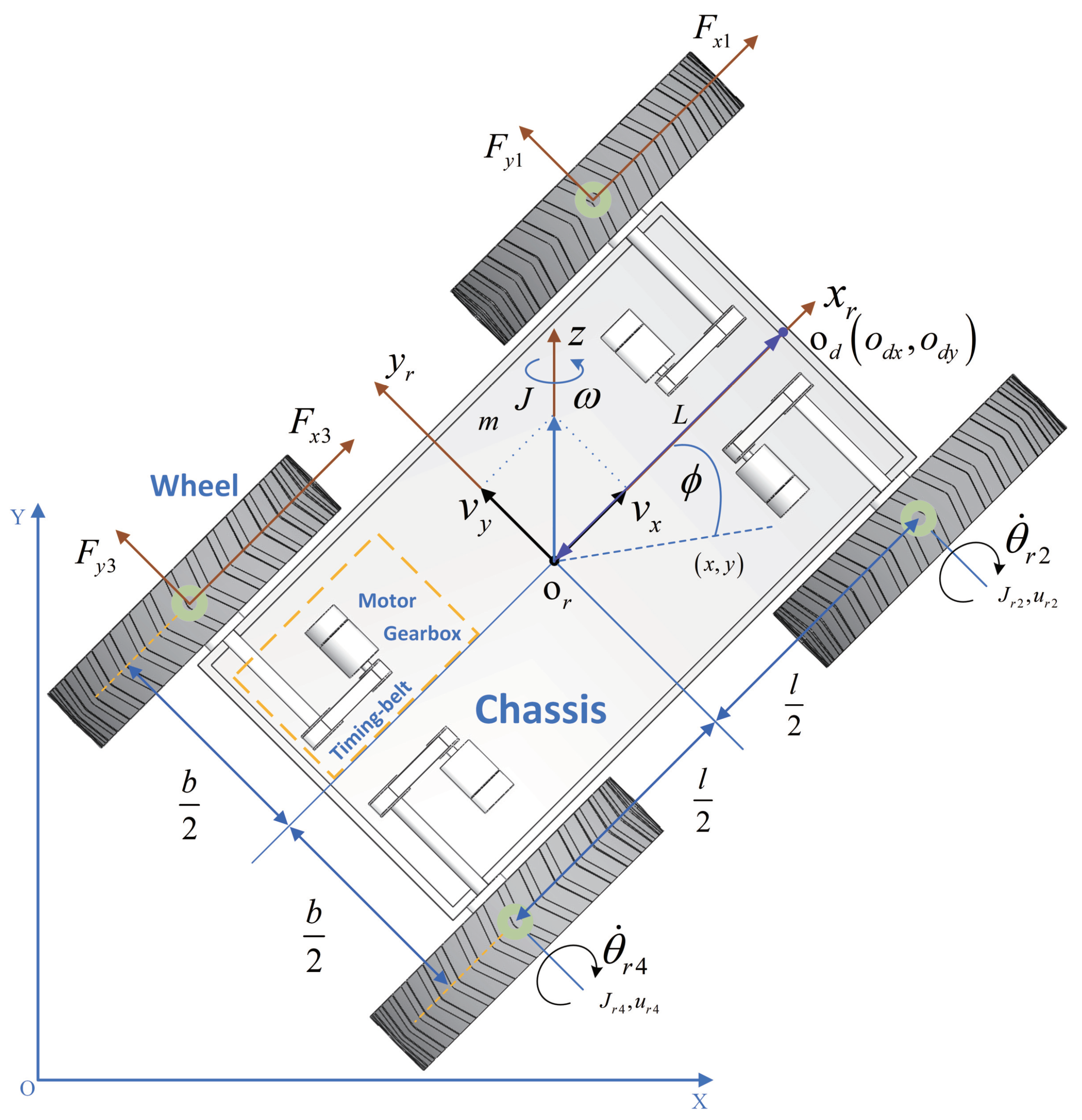
Figure 1 shows the system modeling: O X Y is defined as the reference coordinate system. o r x r y r is the coordinate system attached to the mobile robot. o r is the original point of the coordinate system and is located at the robot’s center of gravity. The coordinate axis x r points to the direction of the chassis movement, and y r is perpendicular to x r . ( x , y ) and ϕ denote the position and rotation angle of the mobile robot coordinate system relative to the reference coordinate system, respectively. v x and v y denote the longitudinal and lateral axes of the mobile robot chassis, respectively. ω denotes the angular velocity of the mobile robot chassis. b denotes the distance between the left and right sides of the mobile robot. The distance is equal between o r and the front and rear wheel axes of the mobile robot due to the mobile robot’s symmetrical design, which denotes one-half of the distance length l of the front and rear wheels. m denotes the weight of the mobile robot, J denotes the rotation inertia of the robot, F x i and F y i represent the longitudinal and lateral forces between the ground and the wheel i, respectively. J r i , θ r i , and u r i represent the rotation inertia, rotation angle, and input force of the driven wheel i, respectively.
In Figure 1, the driven system of each wheel is composed of a timing-belt servo system, and its schematic diagram is shown in Figure 2.
In Figure 2, J m indicates the inertia moment of the motor, and θ m is the rotation angle of the motor and the gearbox input. J g indicates the lumped inertia moment of the belt-driving pulley, and the gearbox output, and θ g is the rotation angle of the gearbox-driven wheel and the belt-driving pulley. J R and θ r represent the lumped inertia moment and the rotation angle of the belt driven pulley and the wheel of the mobile robot, respectively. R 1 and R denote the radius of the driving pulley and driven pulley, respectively.

2.1. Kinematics Modeling

The kinematic model of the mobile robot is as follows [2]
q ˙ = Rv
where q = ( x , y , ϕ ) T and v = v x , v y , ω T represent the vector of the position and velocity for the mobile robot, R is the rotation matrix and is defined as
R = cos ϕ sin ϕ 0 sin ϕ cos ϕ 0 0 0 1 .
In Figure 1, we define o z as the reference position coordinate, the kinematic model of the mobile robot can be rewritten as [29]
o z = [ o z x o z y ]
where o z x = x + L cos ϕ , o z x = x + L cos ϕ , L represents a constant greater than 0. Using Equation (3), we can obtain
o ˙ z = Tv + d k
where the transfer matrix is defined as
T = cos ϕ sin ϕ L sin ϕ sin ϕ cos ϕ L cos ϕ .

2.2. Dynamics Modeling

As seen in Figure 1, the dynamics model of the mobile robot chassis by using the Newton’s law is as follows [3]
m m J v ˙ x v ˙ y ω ˙ T + m ω m ω 0 v y v x ω T = f x f y f ϕ + d x d y d ϕ
where f x = i = 1 4 F x i and f y = i = 1 4 F y i are defined as the combined longitudinal driving force and lateral friction force of the mobile robot, respectively; f ϕ = i = 1 4 A i F i represents the combined yaw torque from the frictions of the wheel-ground interactions with F i = w F x i / 2 l F y i / 2 T , A 1 = 1 1 , A 2 = 1 1 , A 3 = 1 1 , A 4 = 1 1 ; d x , d y , and d ϕ denote disturbances. Thus, combined with the kinematics model (4) and the dynamics model (6), we can obtain a new dynamics formula.
M ¯ o ¨ z + C ¯ o ˙ z = Tu + Td + U
where M = d i a g m m J denotes the inertia matrix, M ¯ = TMT 1 represents the mass matrix, C ¯ = TM T ˙ 1 is the Coriolis matrix, u = f x f y f ϕ T denotes the driving force and yaw moment vector, d = d x d y d ϕ T represents the lumped disturbances, and U is the uncertainties.
Equation (7) has two properties [3].
Property 1.
The matrix M ¯ is symmetric and positive definite.
Property 2.
The matrix M ¯ ˙ 2 C ¯ is a skew-symmetric matrix.
From the dynamics formula (6), the driving force of the motion of the mobile robot is from the wheel–ground interactions [2].
F x i F y i = N i f k S f s x i 2 + s y i 2 s x i 2 + s y i 2 s x i s y i
where f k is the friction coefficient between the wheel and the ground; N i denotes the vertical force of each wheel; S f s x i 2 + s y i 2 = 2 / π a tan 90 s x i 2 + s y i 2 is the approximate function for the dynamics feature of the friction force; s x i and s y i represent the relative velocity of the longitudinal and lateral slip, respectively, which are defined as
s x i = 1 1 ( 1 ) i + 1 r θ ˙ r i v x w ω / 2 T s y i = v y + l f ω , i = 1 , 2 v y l f ω , i = 3 , 4
From Figure 1, the rotational dynamics of each driving wheel is represented as follows.
J r i θ ¨ r i + c r i θ ˙ r i + f r i = u r i r F x i + d r i , i = 1 , 2 , 3 , 4
where c r i denotes the damping coefficient; f r i represents the Coulomb’s friction of the rotation shaft, which is approximated as f r i = A f i S f θ ˙ r i ; u r i denotes the driving torque of each wheel; r is the radius of the wheel; and d r i represents the disturbance and uncertainties. From (6) and Figure 2, the dynamics of the timing-belt servo system is defined as [5]
u r o i = [ k g J m + k t J g + J R ] θ ¨ r i + c t θ ˙ r i + D i
where k g and k t are the transfer coefficient of the gearbox and belt pully, respectively; c t represents the lumped damping coefficient of the gearbox and belt; D i denotes the lumped disturbance and uncertainties.
Moreover, we define three sets of parameters θ = [ θ 1 , θ 2 , θ 5 ] T = [ m , J , d x , d y , d ϕ ] T , θ r = [ θ r 1 , θ r 2 , θ r 5 ] T = [ J r i , c r i , A f i , A i , d r i ] T , and θ t = [ θ t 1 , θ t 2 , θ t 5 ] T = [ J m i , J g i , J R i , c t i , D i ] T represents the linear regression form of the dynamics of the mobile robot’s chassis, wheel, and timing-belt servo system, respectively. Meanwhile, the parameter vector θ is variable due to the changes in the working situations and the mobile robot’s payloads, etc., thus the actual values cannot be exactly known. From the engineering perspective, though influences by various factors (e.g., loads, temperature), the bounds of the parameters (e.g., mass, friction) can usually be decided in advance, and the extent of parametric uncertainties can be predicted [30]. Thus, we have an assumption as follows [10,30].
Assumption A1.
The bound of the unknown parameters are known, which are defined as θ i Ω { θ i : θ i   min θ i θ i   max } , i = 1 , 2 , , 5 , θ r i Ω { θ r i : θ r i   min θ r i θ r i   max } , i = 1 , 2 , , 5 , and θ t i Ω { θ t i : θ t i   min θ t i θ t i   max } , i = 1 , 2 , , 5 .

3. Controller Design

Based on the dynamics model of the mobile robot with timing-belt servo system from Equations (4)–(9), our goal is to design a controller so that the developed mobile robot can track the reference trajectory as well as possible in this paper. To address these problems of the dynamics model uncertainty, redundant driving, and slipping of the four-wheel, independently driven mobile robot with a timing belt servo system, we have developed a controller with a hierarchical control strategy, as shown in Figure 3.
From Figure 3, the hierarchical control strategy is proposed in this paper. First, the adaptive robust control (ARC) law of the chassis can be obtained to achieve the trajectory tracking of the mobile robot at the top level, where the desired driving force and moment of the chassis is generated. Secondly, the control allocation approach can make the driving torque of each wheel solve the redundant driving problem of the mobile robot through the middle layer. Finally, position tracking can be achieved by the adaptive robust control law of the timing-belt servo system in low-level.

3.1. The ARC Law of the Chassis

In order to achieve the goal of trajectory tracking for the mobile robot, let o d t = o d x t , o d y t T be the reference trajectory, e = e x , e y T = o z x t o d x t , o z y t o d y t T be the tracking error, and o z be the current position of the mobile robot. Thus, the function of the slide-mode-like is defined as
s = e ˙ + Λ e
where Λ is a positive diagonal matrix that denotes feedback gain. Thus, from Equation (7) and differentiated Equation (12), we can obtain the error dynamics as follows
M ¯ s ˙ = Tu C ¯ o ˙ z + Td + U M ¯ o ¨ zd + M ¯ Λ e ˙ .
The right side of Equation (13) can be written as a linear regression formula (14).
M ¯ o ¨ zd Λ e ˙ + C ¯ o ˙ z Td = φ T o z , o ˙ z , t θ
where φ is the regressor matrix.
Lemma 1.
The adaptation law with discontinuous projection modification is defined as
θ ^ ˙ i = P r o j θ ^ i Γ η
where θ ^ i is the estimate of the parameter, θ i , Γ > 0 is a diagonal matrix, and η is the adaptation function. Thus, the projection mapping P r o j θ ^ i i is defined as [3]
P r o j θ ^ i i = 0 , if θ ^ i = θ i min and i < 0 0 , if θ ^ i = θ i max and i > 0 i , otherwise
Furthermore, θ ˜ i is defined as the error of θ ^ i minus θ i and can be written as θ ˜ i = θ ^ i θ i .
Moreover, the following conditions are defined.
θ i Ω θ i : θ i min θ i θ i max
θ ˜ i Γ 1 P r o j θ ^ i Γ η η 0 η
where Equations (17) and (18) can guarantee that the projection mapping P r o j θ ^ i i is satisfied for any adaptive function η .
From Equations (13) and (14), we can have the following adaptive robust control law [3,31]
u = T 1 u a + u s , u a = φ T o z , o ˙ z , t θ ^
where u a represents the model compensation term of the adaptive control for the trajectory tracking, and u s is the robust control input that needs to be designed. Thus, the robust control input u s consists of two terms. As follows
u s = u s 1 + u s 2 , u s 1 = k s 1 s
where u s 1 is a linear feedback term with the positive matrix k s 1 and u s 2 is a nonlinear feedback term that is used to address the model uncertainties and to guarantee robust performance. Thus, the following two conditions are suitable for u s 2 .
s T u s 2 φ T θ ˜ + U ε s T u s 2 0
where ε is an arbitrarily small positive parameter.
Here, the adaptation law function is defined as
η = φ s .
Theorem 1.
The proposed controller with the adaptive robust control law and adaptive law can guarantee transient and stable performance.
a. 
Generally, the control input and all state signals of the system are bounded. In addition, we define the positive definite function V t = 1 2 s T M ¯ s , which is bounded and is satisfied by Equation (23).
V t e λ t V 0 + ε λ 1 e λ t
where λ = min 2 σ min K M 1 represents the minimum eigenvalue of a matrix.
b. 
It is assumed that after a finite time t 0 , there is only a parameter uncertainty in the system, i.e., d = 0 , t t 0 . Then, based on the conclusion described ina, the system can also achieve asymptotic tracking with zero error of the stable state. That is, e when t .
(Proof of Theorem 1). 
From the adaptive robust control law, the time derivative of the positive definite function V t is defined as
V ˙ t = s T Tu C ¯ o ˙ z + Td + U M ¯ o ¨ zd + M ¯ Λ e ˙ = s T T u + φ T θ + U = s T K s 1 s + u s 2 φ T θ ˜ + U s T K s 1 s + s T u s 2 φ T θ ˜ + U s T K s 1 s + ε λ V t + ε
The above derivation verifies part a of Theorem 1. Then, the proof of part b in Theorem 1 is as follows.
When d = 0 , t t 0 , select a positive definite function V b t = V t + 1 2 θ ˜ T Γ θ ˜ . From the robust conditions and Equation (18), the time derivative of the positive definite function V b t is defined as
V ˙ b t = V ˙ t + θ ˜ T Γ 1 θ ˜ ˙ = s T T u + φ T θ + U + θ ˜ T Γ 1 θ ˜ ˙ s T K s 1 s s T φ T θ ˜ + θ ˜ T Γ 1 P r o j θ ^ Γ φ s s T K s 1 s + θ ˜ Γ 1 P r o j θ ^ Γ φ s φ s T s T K s 1 s
Since all signals are bounded, it is easy to verify that s ˙ is also bounded, continuous, and consistent. According to Barbalat’s theorem, it is easy to verify part b of Theorem 1, which is proven. □

3.2. The Control Allocation

Although the mobile robot designed in this paper has a damping system, which can avoid the phenomenon of excessive speed due to wheel overhang when the robot passes different ground from the direct power distribution, a novel control allocation approach for driving wheel power distribution is proposed to effectively solve the redundant driving problems. In this subsection, the control allocation approach for the redundant driving of the mobile robot is described. The control allocation strategy mainly achieves the coordinated distribution of the total driving force and torque from the upper-level controller to each driving wheel. In the previous subsection, the total reference driving force u of the mobile robot is obtained by means of the designed adaptive robust controller. To obtain the torque of each driving wheel, we choose the following cost function [32].
J cos t = i = 1 4 W i F x i 2 + F y i 2 N i 2
where W i is the weighted coefficient. In general, the force N i of the vertical direction of each wheel cannot be obtained directly. Then, the nominal force is allocated to actual applications, and the nominal force is defined as N i = m g l / 4 . Furthermore, the cost function has the following constraints.
u x = F x 1 + F x 2 + F x 3 + F x 4
u ϕ = w 2 F x 1 + l 2 F y 1 + w 2 F x 2 + l 2 F y 2 w 2 F x 3 l 2 F y 3 + w 2 F x 4 l 2 F y 4
These constraints are brought into the cost function, and the Lagrange multiplier method is applied to solve the above optimization problem with equation constraints. The Lagrange function is defined as L u x , λ 1 , λ 2 = J cos t + λ 1 u x + λ 2 u ϕ . The partial derivative of the Lagrange function can be derived as
L u x = i = 1 4 2 W i F x i N i 2 + λ 1 + 1 i w 2 λ 2
L λ 1 = u x
L λ 2 = u ϕ
From the above equations, the desired force F x i of each wheel can be obtained. Then, combined with Equation (10), the driving torque u r i can be derived.

3.3. The ARC Law of the Timing-Belt Servo System

From Equations (10) and (11), the torque error of the driving torque of each driving wheel and the output torque of each timing-belt servo system is e r = u r i u r o i . Let e r = 0 have a good control performance. Thus, the following equation can be derived.
J r i k g J m + k t J g + J R θ ¨ r i + c r i c t θ ˙ r i = f r i r F x i + d r i + D i
Define the rotation angle error e θ = θ r θ r d of each driving wheel for the timing-belt servo system. Thus, the function of the slide-mode-like is defined as
s θ = e ˙ θ + ce θ
where c is a positive diagonal matrix used as feedback gain. Thus, from Equation (30) and differentiated Equation (31), we can obtain the error dynamics as follows.
J θ s ˙ θ = u r c θ θ ˙ r + d r + D J θ θ ˙ r d + J θ c e ˙ θ
where J θ = J r k g J m + k t J g + J R , c θ = c r c t , u r = f r r F x .
The right side of Equation (32) can be written as a linear regression form as follows.
J θ θ ˙ r d c e ˙ θ + c θ θ ˙ r d r = Ψ T θ r , θ ˙ r , t θ t
where Ψ is the regressor matrix.
From Equations (32) and (33), the adaption robust control law is defined as
u r = T 1 u ra + u rs , u ra = Ψ T θ r , θ ˙ r , t θ ^ t
where u ra represents the model compensation term of the adaptive control for the trajectory tracking, and u rs is the robust control input that needs to be designed.
Thus, the robust control input u r s consists of two terms. As follows
u rs = u rs 1 + u rs 2 , u rs 1 = k rs 1 s θ
where u rs 1 is a linear feedback term with the positive matrix k rs 1 and u rs 2 is a nonlinear feedback term that is used to address the model uncertainties and to guarantee a robust performance. Thus, the following two conditions are suitable for u rs 2 .
s T u rs 2 φ T θ ˜ + U ε s T u rs 2 0
where ε is an arbitrarily small positive parameter.
In here, the adaptation law function of the timing-belt servo system is defined as
c = φ T s .
The adaptation robust controller of the timing-belt servo system is also met with Theorem 1, and its stability proof can be referred to in Proof 1.

4. Experimental Results

4.1. Experimental Platform

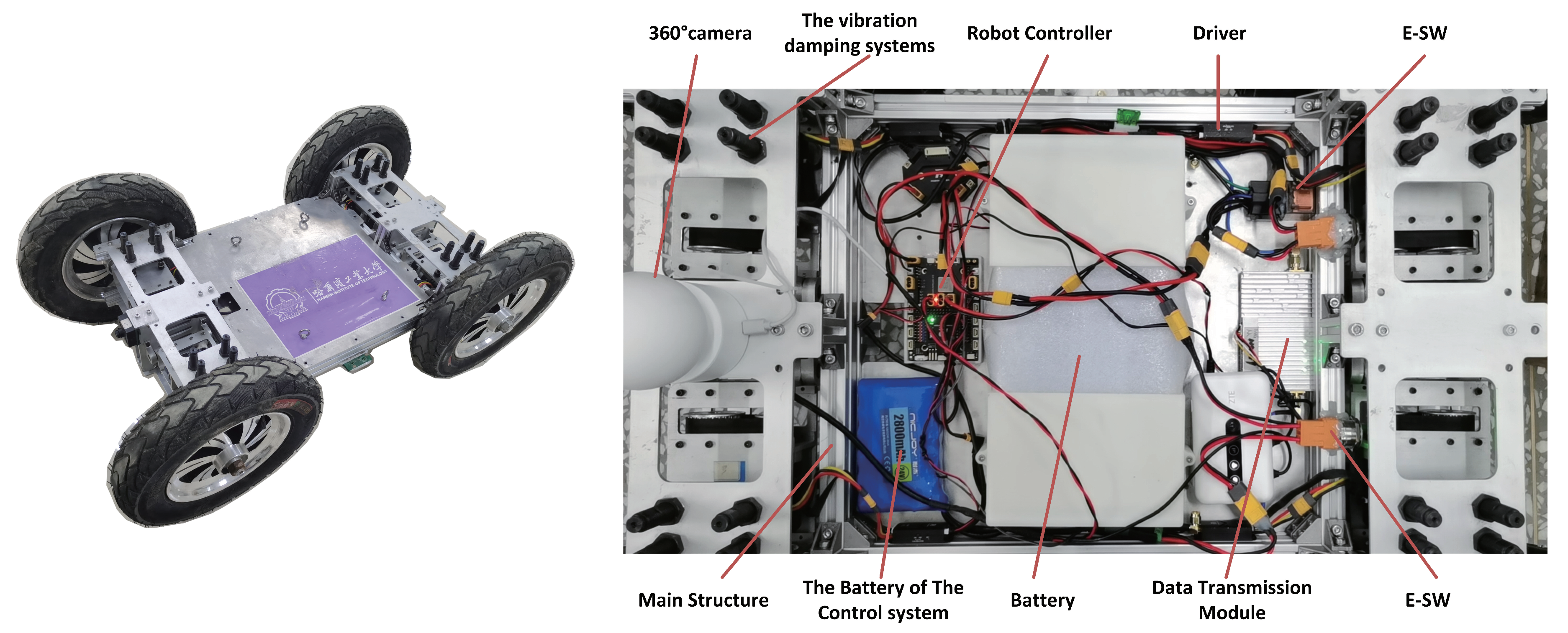
Figure 4 shows the four-wheel, independently driven skid-steer mobile robot with the timing-belt servo system, which is developed by the Institute of Robotics, Harbin Institute of Technology. The mobile robot is composed of the chassis with the vibration damping systems (as shown in Figure 5), timing-belt servo systems (including four brushless DC motors), drivers (with encoder feedback and FOC algorithms), a controller (inside with the ARM Cotex-M4 core) integrated with IMU, a battery (24 V, 5 ah), etc. In order to improve mobility and robust performance on the complicated pavement for the robot, the chassis has simple shock absorbers. To obtain a powerful driving force and torque, each wheel of the mobile robot is driven by an independent timing-belt servo system.
Figure 5 shows the vibration damping system and shock absorber for the robot chassis. The vibration damping system uses a single cross-arm independent suspension that is symmetrical at the top and bottom, with the timing-belt servo mechanism that is hinged to the platform body and can be rotated around the suspension axis. The shock absorber uses a hydraulic buffer element, which is not fixedly connected to the timing-belt servo mechanism and supports the timing-belt servo mechanism by means of upper and lower contact, which ensures that the piston rod is only subjected to axial forces during robot movement. Thus, the timing-belt servo mechanism with the vibration damping system not only makes the robot have the function of a shock absorber and buffer but also makes the robot’s wheels have fuller contact with the ground during the movement.
The control system frame diagram of the mobile robot is shown in Figure 6, the controller of the mobile robot uses the control board based on the ARM Cotex-M4 core and integrates the IMU module, and each timing-belt servo system has an independent driver. The controlling cycle of the mobile robot controller is 10 ms, and the trajectory of the mobile robot is estimated through the IMU and the angle encoder of the timing-belt servo system.
The parameters of the proposed controller design in this paper are shown in Table 1.
Furthermore, the bounds of three sets of linearization parameters are chosen as θ R min = [ 10 , 1.8 , 50 , 50 , 50 ] T , θ R max = [ 30 , 4.2 , 50 , 50 , 50 ] T , θ r min = [ 0.05 , 0.03 , 0.02 , 0 , 0.8 ] T , θ r max = [ 0.15 , 0.05 , 0.15 , 0.3 , 0.8 ] T , θ t min = [ 0.1 , 3.2 , 2.8 , 0.03 , 1 ] T , θ t max = [ 0.7 , 9.6 , 7.2 , 0.07 , 1 ] T .

4.2. Simulation Experimental Results

In order to verify the control performance and trajectory tracking effect of the four-wheel, independently driven skid-steer mobile robot with the timing-belt servo system, which has the vibration damping system, the coordinated controller developed in this paper is compared with the traditional kinematics and dynamics controllers of the mobile robot with the directly driven motor.
  • The kinematics controller
To design the PID controller for the robot kinematics model (3), the rotation angular velocity of the robot-driven wheel is given by the following equation [3].
θ ˙ r i = v x ω b / 2 r i = 1 , 3 v x ω b / 2 r i = 2 , 4
To achieve robot trajectory tracking, a PID calculation of the tracking error is required. Thus, the parameters of the kinematics controller and each timing-belt servo system controller are set to K p = diag 10 , 10 , K i = diag 20 , 20 , K d = diag 0 , 0 and k p = 5.0 , k i = 50 , k d = 0 , respectively.
  • The traditional dynamics controller
From the dynamics modeling (5) and (6), the drive torque of the robot-driven wheels comes from the top-level adaptive robust control output u r i . From the research [29], the direct torque allocation of the driving wheel has the following representation.
u r i = u x u ϕ b / 2 2 r i = 1 , 3 u x + u ϕ b / 2 2 r i = 2 , 4
The parameters of the dynamics controller are set to Λ = diag 5 , 5 . The robust control law is designed as u s 2 = K 2 s , where K 2 represents the combination of linear and robust feedback, K 2 = 4.6 , 4.6 T , and the parameter adaptive law is chosen to be Γ = diag 0 , 0 , 46 , 46 .
  • The proposed coordinated controller
The parameter of the adaptive control law for the proposed coordinated controller is chosen as Λ = diag 5 , 5 . The robust control law is designed as u s 2 = K 2 s , where K 2 represents the combination of linear and robust feedback, K 2 = 4.6 , 4.6 T , and the parameter adaptive law is chosen to Γ = diag 0 , 0 , 46 , 46 . The parameter of the adaptive control law for the timing-belt servo system controller is chosen as Λ = diag 5 , 5 . The robust control law is designed as u rs 2 = K r 2 s , where K r 2 represents the combination of linear and robust feedback, K r 2 = 4.6 , 4.6 T , and the parameter adaptive law is chosen to Γ = diag 0 , 0 , 46 , 46 .
In this paper, compared with the desired trajectory, we design S and inverted octagonal trajectories to verify the performance of the above three controllers by simulation experimental and some experimental measurements iteration.

4.2.1. S Type Trajectory

The S type tracking trajectory used to test the controllers is
o d t = o d x t o d y t = t sin 0.8 t + 0.5 t .
Figure 7 presents the simulation results on S type trajectories tracking performance between the desired trajectory with three controllers, and the comparison is given among the proposed coordinated controller, traditional dynamics controller, and kinematics controller. The root-mean-square value and maximum absolute value of the tracking error [33] on the x-axis, y-axis, and wheel are shown in Figure 8. From Figure 8 and Table 2, it can be seen that the proposed coordinated controller achieves smaller values (smaller than 2 × 10 4 m) of root-mean-square and maximum absolute for the tracking error about the x- and y-axes. It is obvious that the proposed coordinated controller has a better performance than the traditional dynamics controller and kinematics controller. Moreover, the tracking error of the wheel is given in Table 2, which can also reflect the chattering performance of the proposed coordinated controller. Since the kinematics controller is designed based on the assumption that the left and right wheels have the same speed, the same-side wheels need to change the driving force quickly to adapt to the change in the ground friction in order to ensure the same speed, which leads to the phenomenon of mutual pulling of the same-side wheels and causes the robot chattering. For the traditional dynamics controller, since the wheels can be suspended and spun, the robot will also cause a chattering phenomenon when the wheels are constantly changing between suspension and contact. From Figure 8 and Table 2, the errors of the proposed coordination controller are obviously smaller (smaller than 1.6 × 10 4 m) than the other two controllers, and the ability to suppress the chattering phenomenon is also better than the other two.

4.2.2. Inverted Octagonal Type Trajectory

The inverted octagonal type tracking trajectory used to test the controllers is
o d t = o d x t o d y t = 2.5 sin t / 20 π / 2 + 2.5 2.5 cos t / 10 π / 2 .
Furthermore, a simulation experiment for inverted octagonal type trajectory tracking is compared. As shown in Figure 9, the simulation results of the inverted octagonal type trajectory tracking performance between the desired trajectory with three controllers are presented, and a comparison among the proposed coordinated controller, traditional dynamics controller, and kinematics controller is given. Though the inverted octagonal type trajectory is much more complex than the S type; the proposed coordinated controller also has smaller values (smaller than 2.3 × 10 3 m) of root-mean-square and maximum absolute for the tracking error about the x-axis, y-axis, and wheel, which is slightly greater than the S type, and also achieves a better performance than the traditional dynamics controller and kinematics controller, which is presented in Figure 10 and Table 3. It is similar to the tracking error of the wheel about the S type, the proposed coordinated controller also has a good performance on suppressing the chattering phenomenon for inverted octagonal type trajectory tracking.

5. Conclusions

In this paper, a four-wheel, independently driven skid-steer mobile robot with timing-belt servo system, which has a damping module, is developed, and a model-based coordinated control method is proposed, which included chassis kinematics, chassis dynamics, and timing-belt servo system dynamics. The controller we designed consists of three parts. Part one, the adaptive robust controller of the chassis, is based on the dynamics model of the mobile robot, which can generate the combined driving force and torque of the chassis according to the trajectory tracking error. Part two, the control allocation method can convert the combined driving force and torque by the upper-level controller into the driving torque for each timing-belt servo system. Part three, the adaptive robust controller of the timing-belt servo system can complete the output from the driving torque of the timing-belt servo system to the rotation angle of the driving motor and achieve the trajectory tracking control of the mobile robot. Furthermore, theoretical proof of the stability of the designed controller and the tracking performance are also presented and theoretically guaranteed, respectively. In the end, compared with the traditional kinematics and dynamics controller, the simulation experimental results of the coordinated control method we proposed achieves a smaller tracking error and had a better performance. For further research in this paper, the hierarchical control of the robot motion controller considering real application scenes states constraints can also be studied in order to further improve the robot’s motion performance.

Author Contributions

Conceptualization, L.L., H.L. and Y.L.; Data curation, L.L., X.L., X.Z. and B.L.; Funding acquisition, H.L., Y.L. and X.W.; Investigation, X.L. and X.Z.; Methodology, L.L. and B.L.; Project administration, H.L., Y.L. and X.W.; Supervision, H.L., Y.L. and X.W.; Writing—original draft, L.L., X.L., X.Z. and B.L.; Writing—review and editing, L.L., H.L., Y.L. and X.W. All authors have read and agreed to the published version of the manuscript.

Funding

This work is supported in part by the Shenzhen Science Fund for Distinguished Young Scholars (R-CJC20210706091946001), Guangdong Special Branch Plan for Young Talent with Scientific and Technological Innovation (2019TQ05Z111), and the National Natural Science Foundation of China (No. 52265002).

Institutional Review Board Statement

Not applicable.

Informed Consent Statement

Not applicable.

Data Availability Statement

Not applicable.

Conflicts of Interest

Relating to the content of this paper, all authors have no conflict of interest to declare.

References

  1. Ostafew, C.J.; Schoellig, A.P.; Barfoot, T.D. Robust constrained learning-based NMPC enabling reliable mobile robot path tracking. Int. J. Robot. Res. 2016, 35, 1547–1563. [Google Scholar] [CrossRef]
  2. Mohammadpour, E.; Naraghi, M. Robust adaptive stabilization of skid-steer wheeled mobile robots considering slipping effects. Adv. Robot. 2011, 25, 205–227. [Google Scholar] [CrossRef]
  3. Liao, J.; Chen, Z.; Yao, B. Performance-oriented coordinated adaptive robust control for four-wheel independently driven skid-steer mobile robot. IEEE Access 2017, 5, 19048–19057. [Google Scholar] [CrossRef]
  4. Khan, R.; Malik, F.M.; Raza, A.d.; Mazhar, N. Comprehensive study of skid-steer wheeled mobile robots: Development and challenges. Ind. Robot 2021, 48, 142–156. [Google Scholar] [CrossRef]
  5. Yu, Z.; Yang, T.; Ruan, Y.; Xu, T.; Tang, T. A rate-difference disturbance observer control for a timing-belt servo system. IEEE Trans. Ind. Electron. 2021, 69, 11458–11467. [Google Scholar] [CrossRef]
  6. Hace, A.; Jezernik, K.; Sabanovic, A. Smc with disturbance observer for a linear belt drive. IEEE Trans. Ind. Electron. 2007, 54, 3402–3412. [Google Scholar] [CrossRef]
  7. Sabanovic, A.; Sozbilir, O.; Goktug, G.; Sabanovic, N. Sliding mode control of timing-belt servosystem. In Proceedings of the 2003 IEEE International Symposium on Industrial Electronics (Cat. No.03TH8692), Rio de Janeiro, Brazil, 9–11 June 2003; Volume 2, pp. 684–689. [Google Scholar] [CrossRef]
  8. Minh, V.T.; Tamre, M.; Sekhri, E. Modeling and robust control algorithms for a linear belt driven system. Open Comput. Sci. 2018, 8, 142–153. [Google Scholar] [CrossRef]
  9. Zhu, H.; Zhu, W.D.; Fan, W. Dynamic modeling, simulation and experiment of power transmission belt drives: A systematic review. J. Sound Vib. 2021, 491, 115759. [Google Scholar] [CrossRef]
  10. Ryu, J.C.; Agrawal, S.K. Differential flatness-based robust control of mobile robots in the presence of slip. Int. J. Robot. Res. 2011, 30, 463–475. [Google Scholar] [CrossRef]
  11. Huang, J.; Wen, C.; Wang, W.; Jiang, Z.-P. Adaptive output feedback tracking control of a nonholonomic mobile robot. Automatica 2014, 50, 821–831. [Google Scholar] [CrossRef]
  12. Deng, M.; Inoue, A.; Sekiguchi, K.; Jiang, L. Two-wheeled mobile robot motion control in dynamics environments. Robot. Comput.-Integr. Manuf. 2010, 26, 268–272. [Google Scholar] [CrossRef]
  13. Sun, W.; Tang, S.; Gao, H.; Zhao, J. Two time-scale tracking control of nonholonomic wheeled mobile robots. IEEE Trans. Control Syst. Technol. 2016, 24, 2059–2069. [Google Scholar] [CrossRef]
  14. Low, C.B.; Wang, D. GPS-based tracking control for a car-like wheeled mobile robot with skidding and slipping. IEEE/ASME Trans. Mechatron. 2008, 13, 480–484. [Google Scholar]
  15. Li, B.; Fang, Y.; Zhang, X. Visual servo regulation of wheeled mobile robots with an uncalibrated onboard camera. IEEE/ASME Trans. Mechatron. 2016, 21, 2330–2342. [Google Scholar] [CrossRef]
  16. Yoo, S.J. Adaptive tracking control for a class of wheeled mobile robots with unknown skidding and slipping. IET Control Theory Appl. 2010, 4, 2109–2119. [Google Scholar] [CrossRef]
  17. Yao, J.; Jiao, Z.; Ma, D.; Yan, L. High-accuracy tracking control of hydraulic rotary actuators with modeling uncertainties. IEEE/ASME Trans. Mechatron. 2014, 19, 633–641. [Google Scholar] [CrossRef]
  18. Li, Z.; Deng, J.; Lu, R.; Xu, Y. Trajectory-tracking control of mobile robot systems incorporating neural-dynamics optimized model predictive approach. IEEE Trans. Syst. Man Cybern. Syst. 2016, 46, 740–749. [Google Scholar] [CrossRef]
  19. Hu, C.; Wang, R.; Yan, F. Composite nonlinear feedback control for path following of four-wheel independently actuated autonomous ground vehicles. IEEE Trans. Intell. Transp. Syst. 2016, 17, 2063–2074. [Google Scholar]
  20. Chen, Y.; Wang, J. Adaptive energy-efficient control allocation for planar motion control of over-actuated electric ground vehicles. IEEE Trans. Control Syst. Technol. 2014, 22, 1362–1373. [Google Scholar]
  21. Chen, Y.; Wang, J. Design and experimental evaluations on energy efficient control allocation methods for over-actuated electric vehicles: Longitudinal motion case. IEEE/ASME Trans. Mechatron. 2014, 19, 538–548. [Google Scholar] [CrossRef]
  22. Wang, Y.; Fujimoto, H.; Hara, S. Driving force distribution and control for EV with four in-wheel motors: A case study of acceleration on split-friction surfaces. IEEE Trans. Ind. Electron. 2017, 64, 3380–3388. [Google Scholar] [CrossRef]
  23. Sun, W.; Zhang, Y.; Huang, Y.; Gao, H.; Kaynak, O. Transient-performance-guaranteed robust adaptive control and its application to precision motion control systems. IEEE Trans. Ind. Electron. 2016, 63, 6510–6518. [Google Scholar] [CrossRef]
  24. Morawiec, M. The adaptive backstepping control of permanent magnet synchronous motor supplied by current source inverter. IEEE Trans. Ind. Inform. 2013, 9, 1047–1055. [Google Scholar] [CrossRef]
  25. Feng, Z.; Zheng, W.X. On extended dissipativity of discrete-time neural networks with time delay. IEEE Trans. Neural Netw. Learn. Syst. 2015, 26, 3293–3300. [Google Scholar] [CrossRef] [PubMed]
  26. Ma, J.; Chen, S.L.; Kamaldin, N.; Teo, C.S.; Tay, A.; Al Mamun, A.; Tan, K.K. Integrated mechatronic design in the flexure-linked dualdrive gantry by constrained linear quadratic optimization. IEEE Trans. Ind. Electron. 2018, 65, 2408–2418. [Google Scholar] [CrossRef]
  27. Kommuri, S.K.; Defoort, M.; Karimi, H.R.; Veluvolu, K.C. A robust observer-based sensor fault-tolerant control for pmsm in electric vehicles. IEEE Trans. Ind. Electron. 2016, 63, 7671–7681. [Google Scholar] [CrossRef]
  28. Chen, Z.; Pan, Y.; Gu, J. Integrated adaptive robust control for multilateral teleoperation systems under arbitrary time delays. Int. J. Robust Nonlinear Control 2016, 26, 2708–2728. [Google Scholar] [CrossRef]
  29. Rodrłguez-Seda, E.J.; Tang, C.; Spong, M.W.; Stipanovic, D.; An, M. Trajectory tracking with collision avoidance for nonholonomic vehicles with acceleration constraints and limited sensing. Int. J. Robot. Res. 2014, 33, 1569–1592. [Google Scholar] [CrossRef]
  30. Hu, C.; Yao, B.; Wang, Q. Coordinated adaptive robust contouring control of an industrial biaxial precision gantry with cogging force compensations. IEEE Trans. Ind. Electron. 2010, 57, 1746–1754. [Google Scholar]
  31. Chen, Z.; Yao, B.; Wang, Q. μ-synthesis-based adaptive robust control of linear motor driven stages with high-frequency dynamics: A case study. IEEE/ASME Trans. Mechatron. 2015, 20, 1482–1490. [Google Scholar] [CrossRef]
  32. Mokhiamar, O.; Abe, M. Simultaneous optimal distribution of lateral and longitudinal tire forces for the model following control. J. Dyn. Syst. Meas. Control 2004, 126, 753–763. [Google Scholar] [CrossRef]
  33. Wang, R.; Jing, H.; Yan, F.; Karimi, H.R.; Chen, N. Optimization and finite-frequency h control of active suspensions in in-wheel motor driven electric ground vehicles. J. Frankl. Inst. 2015, 352, 468–484. [Google Scholar] [CrossRef]
Figure 1. Top view of the four-wheel, independent skid-steer mobile robot with timing-belt servo system.
Electronics 12 00699 g001
Figure 2. Schematic diagram of the timing-belt servo system.
Electronics 12 00699 g002
Figure 3. The overall control architecture.
Electronics 12 00699 g003
Figure 4. The mobile robot.
Electronics 12 00699 g004
Figure 5. The vibration damping system and the shock absorber of the chassis.
Electronics 12 00699 g005
Figure 6. The block diagram of the mobile robot control system.
Electronics 12 00699 g006
Figure 7. The simulation results for the S type trajectory tracking performance.
Electronics 12 00699 g007
Figure 8. The S type trajectory tracking error performance.
Electronics 12 00699 g008
Figure 9. The simulation results for the inverted octagonal type trajectory tracking performance.
Electronics 12 00699 g009
Figure 10. The inverted octagonal type trajectory tracking error performance.
Electronics 12 00699 g010
Table 1. The key parameters of the mobile robot.
NO.ParameterSymbolValueUnit
1Chassis Weightm18kg
2Chassis InertiaJ2.12kg ∗ m 2
3Chassis Lengthl0.6m
4Chassis Widthb0.4m
5Wheel Radiusr0.15m
6Driven Pulley RadiusR0.06m
7Driving Pulley Radius R 1 0.03m
8Gearbox Ratio k g 20
9Belt Reduction Ratio k t 2.0
Table 2. The S type trajectory tracking error values for the three controllers.
Controller | | e x | | rms | | e x | | max | | e y | | rms | | e y | | max | | e r | | rms | | e r | | max
Kinematics 3.21 × 10 4 3.81 × 10 4 2.46 × 10 4 2.76 × 10 4 2.22 × 10 4 2.77 × 10 4
Dynamics 2.53 × 10 4 2.71 × 10 4 1.82 × 10 4 2.12 × 10 4 1.56 × 10 4 2.21 × 10 4
Proposed 1.47 × 10 4 1.52 × 10 4 1.41 × 10 4 1.88 × 10 4 1.21 × 10 4 1.57 × 10 4
Table 3. The inverted octagonal type trajectory tracking error values for three controllers.
Controller | | e x | | rms | | e x | | max | | e y | | rms | | e y | | max | | e r | | rms | | e r | | max
Kinematics 3.71 × 10 3 4.31 × 10 3 2.96 × 10 3 3.26 × 10 3 2.72 × 10 3 3.27 × 10 3
Dynamics 2.93 × 10 3 3.22 × 10 3 2.32 × 10 3 2.62 × 10 3 2.06 × 10 3 2.61 × 10 3
Proposed 1.87 × 10 3 1.92 × 10 3 1.81 × 10 3 2.28 × 10 3 1.61 × 10 3 2.07 × 10 3
Disclaimer/Publisher’s Note: The statements, opinions and data contained in all publications are solely those of the individual author(s) and contributor(s) and not of MDPI and/or the editor(s). MDPI and/or the editor(s) disclaim responsibility for any injury to people or property resulting from any ideas, methods, instructions or products referred to in the content.

