A Study on Characteristic Mode Equations of Radiation Problems Contrasted with Scattering Problems for Dielectric Bodies

Abstract

This paper is concerned with the extractions of electromagnetic characteristic modes (CMs) for lossless dielectric bodies, for which spurious modes are prone to generate using the traditional definition of CMs based on the Poggio–Miller–Chang–Harrington–Wu–Tsai (PMCHWT) equations. It is found that the impedance matrix of PMCHWT equations cannot distinguish (i) which domain is the dielectric body and which domain is the background and (ii) from which domain the excitation source was applied. If the system is taken as a scattering problem, the spurious modes are solutions to a reverse media problem, i.e., exchanging the media of the dielectric body and the background space. However, if the system is taken as a radiation problem, no appropriate CMs that meet the specified boundary conditions are obtained. These phenomena indicate that CMs developed from scattering systems are not suitable for radiation systems. To clarify the issue, four cases with reverse media and with excitation sources in either domain are examined. The four cases are distinct in essence, but the PMCHWT equations cannot distinguish them. As a result, definitions of CMs for the four cases should be given along with their specific boundary conditions. Especially, the CMs for the radiation problems we consider here show that the excitation source inside the material object should be properly defined in order to be distinguished from scattering problems.

1. Introduction

The theory of characteristic modes (TCM) based on the electric field integral equation (EFIE) for a perfectly electric conductor (PEC) was proposed by Harrington and Mautz in 1971 [1]. The resulting characteristic modes (CMs) are not dependent on the excitation source but on the structure and material of the object. Due to this superior property, it has been employed as a great potential analysis tool for antenna design [2], such as in the reduction of the cross-sections of radar antenna [3], the improvement of multiple-input-multiple-output antenna [4], etc.

Subsequently, TCM was generalized to material objects by employing a volume integral equation (VIE) [5] and a surface integral equation (SIE) [6]. Unfortunately, the SIE-based TCM was reported to generate spurious modes [7]. In order to remove these spurious modes, there are some valuable formulations [8,9,10,11,12,13], including building a dependent relationship between equivalent electric and magnetic currents [8,9,10,11,12,13,14] and making the right-hand side of the generalized eigenvalue equation (GEE) related to only radiated power [11,12,13]. Thus far, the spurious modes have almost been suppressed.

However, few researchers have discussed why the spurious modes appear when using SIE-based TCM, especially the traditional TCM based on the symmetric PMCHWT by Chang and Harrington [6] (CH-sPMCHWT-TCM). Miers and Lau [15] think that internal resonance may partly explain this phenomenon because sPMCHWT could not remove internal resonance. However, the spurious modes still exist when sPMCHWT is changed to asymmetric PMCHWT (CH-PMCHWT-TCM). Thus, the internal resonance should not be responsible for the spurious modes [16]. As a remedy, some researchers [8,10,16] found that the spurious (non-physical) modes do not obey the dependent relationship of equivalent electric and magnetic currents, while the physical modes do. Namely, the dependent relationship can be taken as a post-process technology to separate the physical and non-physical modes. Bernabeu-Jiménez et al. [17] pointed out that the spurious modes can be excited by an internal source for the infinite lossless dielectric cylinder, which means that the spurious modes may exist in reality and are renamed as non-radiation modes. However, the spurious modes of lossless material objects are found to be coincident with the CMs of the reverse problem, where the material parameters of the object and the background are swapped [18].

The CMs for material objects are independent of the excitation source, so they are expected to be applicable to analyses of both scattering and radiation problems. It is noted that existing SIE-based formulations are essentially established in the scattering system framework. Therefore, the formulations are suitable for scattering problems indisputably. It is uncertain whether the resulting CMs include those of radiation problems, especially when the sources are inside the objects. Recently, our previous work [19] revealed that EFIE-based TCM [1] is not appropriate for wave-port-fed transmitting PEC structures.

There are some existing works that apply TCM to deal with real antenna systems;, mainly by using a mixed potential integral equation with the spatial domain Green’s functions of multilayer mediums [20,21] or volume and surface integral equations [22,23], other than the forementioned SIE-based TCM. It is worth mentioning that the radiation problem we will consider is that the source is inside the material object.

In this paper, we will discuss four physical models with reverse media and with the excitation source in either domain in order to demonstrate the reason why CH-PMCHWT-TCM is prone to generate spurious modes. We find that the impedance operator of the PMCHWT equation mixes the two different media without specified excitation and is also the same whether the excitation is inside or outside. For this reason, we define the CMs of the four cases by using specified boundary conditions.

2. Traditional Theory for Four Physical Problems

It is known that the PMCHWT equation solves a mixed problem with two different media and gives a unique solution for a specified excitation. However, for a characteristic mode problem that is independent of the excitation, if improperly defined, the generalized eigenvalue equation (GEE) may not be able to distinguish (i) the two domains if their media are reversed and (ii) the excitation from inside or outside. Let us start with the four cases, as shown in Figure 1. Cases (A) and (B) are scattering problems to be excited from the outside, but the media are reversed. Cases (C) and (D) are radiation problems to be excited from the inside.

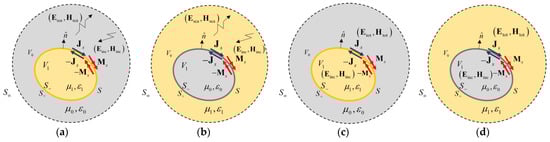
Figure 1. Illustration of scattering and radiation problems in reverse media. (a) Problem (A); (b) problem (B); (c) problem (C); (d) problem (D).

For the scattering problem (A), in terms of the extinction theorem, the surface equivalent currents $(J_s,M_s)$ would generate $(-E^{inc},-H^{inc})$ in V₁ if V₁ were filled with the same medium as in V₂, while $(-J_s,-M_s)$ would generate zero fields in V₂ if V₂ were filled with the same medium as in V₁, i.e.,

$$-{\eta }_2{\mathcal{L}}_2(J_s)+{\mathcal{K}}_2(M_s)=-E^{inc}, r\in V_1$$

(1)

$$-{\zeta }_2{\mathcal{L}}_2(M_s)-{\mathcal{K}}_2(J_s)=-H^{inc}, r\in V_1$$

(2)

$$-{\eta }_1{\mathcal{L}}_1(-J_s)+{\mathcal{K}}_1(-M_s)=0, r\in V_2$$

(3)

$$-{\zeta }_1{\mathcal{L}}_1(-M_s)-{\mathcal{K}}_1(-J_s)=0, r\in V_2$$

(4)

where ${\eta }_i=1/{\zeta }_i=\sqrt{{\mu }_i/{\epsilon }_i}$, and the operators are defined as

$${\mathcal{L}}_i(X)=j{k}_i{\displaystyle \underset{S}{\oint }\left[G_i(R)X(r^{\prime })+\frac{1}{k_i{}^2}\nabla G_i(R){\nabla }^{\prime }·X(r^{\prime })\right]d{S}^{\prime }}$$

(5)

$${\mathcal{K}}_i(X)={\displaystyle \underset{S}{\oint }X(r^{\prime })\times \nabla G_i(R)d{S}^{\prime }}.$$

(6)

When the observation points approach the surface S from the inside and outside, respectively, we would recognize that ${\mathcal{K}}_2(X)={\tilde{\mathcal{K}}}_2(X)-\frac{1}{2}\widehat{n}\times X$ and ${\mathcal{K}}_1(X)={\tilde{\mathcal{K}}}_1(X)+\frac{1}{2}\widehat{n}\times X$, with ${\tilde{\mathcal{K}}}_i(X)$ being the principal-value part of ${\mathcal{K}}_i(X)$. After the discretization of (1)–(4) by the Galerkin method with the RWG basis functions $\left\{f_n(r),n=1,\cdots ,N\right\}$ and singularity treatment [24], we can obtain

$$\left[\begin{array}{cc}{\eta }_2{\mathbb{L}}_2& -{\tilde{\mathbb{K}}}_2+\frac{1}{2}\mathbb{C}\\ {\tilde{\mathbb{K}}}_2-\frac{1}{2}\mathbb{C}& {\zeta }_2{\mathbb{L}}_2\end{array}\right]\left[\begin{array}{c}\mathbb{J}\\ \mathbb{M}\end{array}\right]=\left[\begin{array}{c}{\mathbb{E}}^{inc}\\ {\mathbb{H}}^{inc}\end{array}\right]$$

(7)

$$\left[\begin{array}{cc}{\eta }_1{\mathbb{L}}_1& -{\tilde{\mathbb{K}}}_1-\frac{1}{2}\mathbb{C}\\ {\tilde{\mathbb{K}}}_1+\frac{1}{2}\mathbb{C}& {\zeta }_1{\mathbb{L}}_1\end{array}\right]\left[\begin{array}{c}\mathbb{J}\\ \mathbb{M}\end{array}\right]=0$$

(8)

where the matrix elements are

$${[{\mathbb{L}}_i]}_{m,n}=⟨f_m(r),{\mathcal{L}}_i(f_n(r^{\prime }))⟩$$

(9)

$${[{\mathbb{K}}_i]}_{m,n}=⟨f_m(r),{\mathcal{K}}_i(f_n(r^{\prime }))⟩$$

(10)

$${[\mathbb{C}]}_{m,n}=⟨f_m(r),\widehat{n}\times f_n(r)⟩.$$

(11)

By denoting

$${\tilde{\mathbb{Z}}}_i=\left[\begin{array}{cc}{\eta }_i{\mathbb{L}}_i& -{\tilde{\mathbb{K}}}_i\\ {\tilde{\mathbb{K}}}_i& {\zeta }_i{\mathbb{L}}_i\end{array}\right],\mathbb{D}=\left[\begin{array}{cc}0& \mathbb{C}\\ -\mathbb{C}& 0\end{array}\right]$$

(12)

$$\mathbb{F}=\left[\begin{array}{c}\mathbb{J}\\ \mathbb{M}\end{array}\right],\mathbb{V}=\left[\begin{array}{c}{\mathbb{E}}^{inc}\\ {\mathbb{H}}^{inc}\end{array}\right]$$

(13)

we may rewrite (7)–(8) compactly as

$${\tilde{\mathbb{Z}}}_2^{+}\mathbb{F}=\mathbb{V}$$

(14)

$${\tilde{\mathbb{Z}}}_1^{-}\mathbb{F}=0$$

(15)

with

$${\tilde{\mathbb{Z}}}_i^{\pm }={\tilde{\mathbb{Z}}}_i\pm \frac{1}{2}\mathbb{D},i=1,2.$$

(16)

Adding (15) to (14), one obtains the classical PMCHWT equation

$$\tilde{\mathbb{Z}} \mathbb{F}=\mathbb{V}$$

(17)

where $\tilde{\mathbb{Z}}={\tilde{\mathbb{Z}}}_1^{-}+{\tilde{\mathbb{Z}}}_2^{+}={\tilde{\mathbb{Z}}}_1+{\tilde{\mathbb{Z}}}_2$. Make ${\tilde{\mathbb{Z}}}_i={\tilde{\mathbb{R}}}_i+j{\tilde{\mathbb{X}}}_i$, with

$${\tilde{\mathbb{R}}}_i=\frac{1}{2}\left({\tilde{\mathbb{Z}}}_i+{\tilde{\mathbb{Z}}}_i^H\right),{\tilde{\mathbb{X}}}_i=\frac{1}{2j}\left({\tilde{\mathbb{Z}}}_i-{\tilde{\mathbb{Z}}}_i^H\right)$$

(18)

in which the superscript “H” denotes the Hermitian transpose. As one of the traditional ways, the GEE is defined by $\tilde{\mathbb{Z}}{\mathbb{F}}_n=(1+j{\lambda }_n)\left({\tilde{\mathbb{R}}}_1+{\tilde{\mathbb{R}}}_2\right){\mathbb{F}}_n$, i.e.,

$$\left({\tilde{\mathbb{X}}}_1+{\tilde{\mathbb{X}}}_2\right){\mathbb{F}}_n={\lambda }_n\left({\tilde{\mathbb{R}}}_1+{\tilde{\mathbb{R}}}_2\right){\mathbb{F}}_n.$$

(19)

which is the so-called CH-PMCHWT-CM [6,16]. Unfortunately, this formulation would generate many spurious modes, as reported in [7,8,9,10,11,12].

To identify the reason, we may check the solutions with the boundary condition (15) and find that these spurious modes do not observe it, as reported in [16]. This means that these modes are not physical solutions to scattering problem (A). Then, what boundary condition do these spurious modes satisfy? There exist problems (B), (C) and (D), as displayed in Figure 1, all of which can obtain a GEE similar to (19) if following the conventional way, as discussed below.

For the scattering problem (B) in Figure 1, the corresponding equations to (14)–(15) are

$${\tilde{\mathbb{Z}}}_1^{+}\mathbb{F}=\mathbb{V}$$

(20)

$${\tilde{\mathbb{Z}}}_2^{-}\mathbb{F}=0.$$

(21)

Adding these two equations, one obtains the same PMCHWT equation as (17), and then the same GEE as (19), but the boundary condition (BC) needing to meet is (21), not (15).

For the radiation problem (C) in Figure 1, by using the same procedure as described for problem (A), we can obtain the corresponding equations to (14)–(15) as

$${\tilde{\mathbb{Z}}}_1^{-}\mathbb{F}=-\mathbb{V}$$

(22)

$${\tilde{\mathbb{Z}}}_2^{+}\mathbb{F}=0.$$

(23)

Again, the addition of these two equations gives the same PMCHWT equation as (17) and the same GEE as (19), but the BC needing to meet is (23).

Finally, for radiation problem (D), the corresponding equations to (14)–(15) are

$${\tilde{\mathbb{Z}}}_2^{-}\mathbb{F}=-\mathbb{V}$$

(24)

$${\tilde{\mathbb{Z}}}_1^{+}\mathbb{F}=0.$$

(25)

It is apparent that the PMCHWT and GEE equations for this problem are also (17) and (19), respectively; however, the BC needing to be met becomes (25).

In summary, the PMCHWT Equation (17) and the GEE (19) cannot distinguish the four cases in Figure 1. One must use one of the boundary conditions (BCs) of (15), (21), (23), or (25) to select suitable modes.

Referring to (8), the solution of (15) is

$$\mathbb{J}={\zeta }_1{\mathbb{S}}_1^{+}\mathbb{M}, \mathrm{or} \mathbb{M}=-{\eta }_1{\mathbb{S}}_1^{+}\mathbb{J}$$

(26)

with

$${\mathbb{S}}_i^{\pm }={({\mathbb{L}}_i)}^{-1}({\tilde{\mathbb{K}}}_i\pm \frac{1}{2}\mathbb{C}), i=1,2.$$

(27)

Similarly, solutions of (21), (23), and (25) can also been obtained, respectively, as follows:

$$\mathbb{J}={\zeta }_2{\mathbb{S}}_2^{+}\mathbb{M}, \mathrm{or} \mathbb{M}=-{\eta }_2{\mathbb{S}}_2^{+}\mathbb{J}$$

(28)

$$\mathbb{J}={\zeta }_2{\mathbb{S}}_2^{-}\mathbb{M}, \mathrm{or} \mathbb{M}=-{\eta }_2{\mathbb{S}}_2^{-}\mathbb{J}$$

(29)

$$\mathbb{J}={\zeta }_1{\mathbb{S}}_1^{-}\mathbb{M}, \mathrm{or} \mathbb{M}=-{\eta }_1{\mathbb{S}}_1^{-}\mathbb{J}.$$

(30)

There are two schemes to judge which one of the four problems the modes ${\mathbb{F}}_n$ solved from GEE (19) satisfy. One way is to submit the found characteristic modes ${\mathbb{F}}_n$ into (15), (21), (23), or (25) and then see whether the corresponding error of matrix-vector multiplication $[{\mathbb{Z}}_k^{\pm }][{\mathbb{F}}_n],k=0,1$ is sufficiently small. The error is defined as

$$error=\frac{\sqrt{{\displaystyle \sum _{i=1}^{2N}{\left|{\displaystyle \sum _{j=1}^{2N}{[{\mathbb{Z}}_k^{\pm }]}_{i,j}{[{\mathbb{F}}_n]}_j}\right|}^2}}}{\sqrt{{\displaystyle \sum _{j=1}^{2N}{\left|{[{\mathbb{F}}_n]}_j\right|}^2}}}, k=0,1$$

(31)

Another way is to calculate the correlation coefficient of the known and new characteristic electric and magnetic currents as in [16], where the known characteristic modal electric and magnetic currents $\left(J_n,M_n\right)$ are constructed by ${\mathbb{F}}_n$, and the new modal electric $J_n^{\prime }$ are obtained by submitting the known characteristic magnetic currents $M_n$ into (26), (28), (29) or (30), i.e., $J_n^{\prime }=J_n^{\prime }\left(M_n\right)$. Analogously, the new magnetic currents $M_n^{\prime }$($M_n^{\prime }=M_n^{\prime }\left(J_n\right)$) are obtained from the known $J_n$. For brevity, the resulting new modal currents computed from (26), (28)–(30) are denoted as $\left({\left(J_n^{\prime }\right)}_{\mathrm{K}},{\left(M_n^{\prime }\right)}_{\mathrm{K}}\right)$ with symbol ‘K’ = ’A’, ’B’, ’C’ or ’D’, respectively. For instance, if the n-th mode is the solution of problem (A), $\left({(J_n^{\prime })}_{\mathrm{A}},{\left(M_n^{\prime }\right)}_{\mathrm{A}}\right)$ should be the same as $\left(J_n,M_n\right)$. A similar scheme applies to other problems. In order to judge the equality, we can define the correlation coefficients as

$$\mathrm{K}-{\rho }_J\left({\mathbf{J}}_n,{\left({\mathbf{J}}_n^{\prime }\right)}_{\mathrm{K}}\right)=\frac{\left|⟨{\mathbf{J}}_n^{\prime },{\left({\mathbf{J}}_n^{\prime }\right)}_{\mathrm{K}}⟩\right|}{\sqrt{⟨{\mathbf{J}}_n,{\left({\mathbf{J}}_n^{\prime }\right)}_{\mathrm{K}}⟩}\sqrt{⟨{\left({\mathbf{J}}_n^{\prime }\right)}_{\mathrm{K}},{\left({\mathbf{J}}_n^{\prime }\right)}_{\mathrm{K}}⟩}}·\min \left\{\frac{⟨{\mathbf{J}}_n,{\mathbf{J}}_n⟩}{⟨{\left({\mathbf{J}}_n^{\prime }\right)}_{\mathrm{K}},{\left({\mathbf{J}}_n^{\prime }\right)}_{\mathrm{K}}⟩},\frac{⟨{\left({\mathbf{J}}_n^{\prime }\right)}_{\mathrm{K}},{\left({\mathbf{J}}_n^{\prime }\right)}_{\mathrm{K}}⟩}{⟨{\mathbf{J}}_n,{\mathbf{J}}_n⟩}\right\}$$

(32)

$$\mathrm{K}-{\rho }_M\left({\mathbf{M}}_n,{\left({\mathbf{M}}_n^{\prime }\right)}_{\mathrm{K}}\right)=\frac{\left|⟨{\left({\mathbf{M}}_n^{\prime }\right)}_{\mathrm{K}},{\left({\mathbf{M}}_n^{\prime }\right)}_{\mathrm{K}}⟩\right|}{\sqrt{⟨{\mathbf{M}}_n,{\mathbf{M}}_n⟩}\sqrt{⟨{{\left({\mathbf{M}}_n^{\prime }\right)}_{\mathrm{K}}}_n,{\left({\mathbf{M}}_n^{\prime }\right)}_{\mathrm{K}}⟩}}·\min \left\{\frac{⟨{\mathbf{M}}_n,{\mathbf{M}}_n⟩}{⟨{\left({\mathbf{M}}_n^{\prime }\right)}_{\mathrm{K}},{\left({\mathbf{M}}_n^{\prime }\right)}_{\mathrm{K}}⟩},\frac{⟨{\left({\mathbf{M}}_n^{\prime }\right)}_{\mathrm{K}},{\left({\mathbf{M}}_n^{\prime }\right)}_{\mathrm{K}}⟩}{⟨{\left({\mathbf{M}}_n^{\prime }\right)}_{\mathrm{K}},{\left({\mathbf{M}}_n^{\prime }\right)}_{\mathrm{K}}⟩}\right\}$$

(33)

One mode is identified to satisfy one of the four problems if both of its correlation coefficients $\mathrm{K}-{\rho }_J$ and $\mathrm{K}-{\rho }_M$ are close to 1 for ‘K’ = ’A’, ’B’, ’C’ and ’D’.

One example is given to observe which one of the four cases the modes solved from GEE (19) satisfy. A cubic dielectric resonator (DR) (a = b = c = 25.4 mm) in [15] is considered since it has been frequently applied as a verified example [11,12,13,14]. Its constitutive parameters are ${\epsilon }_{r1}=9.4$ and ${\mu }_{r1}=1.0$, and the background is the air, i.e., ${\epsilon }_{r2}=1.0$ and ${\mu }_{r2}=1.0$. The cubic DR is meshed as 528 triangular patches.

The real part of characteristic eigenvalues solved from GEE (19) is displayed in Figure 2, with a frequency range from 2.0 GHz to 4.5 GHz. Good agreements can be observed with the results in [18]. The solid red lines represent the so-called physical characteristic modes of scattering problem (A), and the black lines denote the spurious modes of scattering problem A.

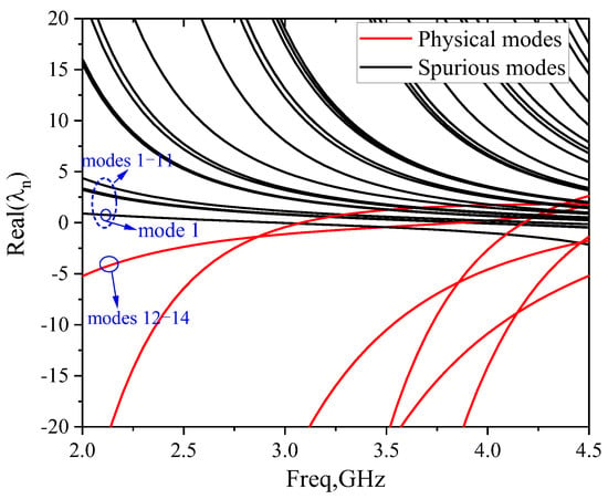
Figure 2. The real parts of characteristic eigenvalues of the first 150 lower order modes in the frequency range from 2.0 GHz to 4.5 GHz.

In order to understand the underlying physical meaning of these spurious modes, we apply the BCs of the four problems (A), (B), (C), and (D). The errors and correlation coefficients of the first 70 lower-order modes at a frequency point of 2.0 GHz are demonstrated in Figure 3. It is noted that the evaluated standard is less than 1 × 10⁻⁶ for the error scheme, while the standard is bigger than 0.95 for the correlation coefficient scheme. It is obviously observed that some modes of the first 70 modes satisfy the BC of scattering problem (A), but some modes satisfy the BC of scattering problem (B). For instance, the correlation coefficients $\left(\mathrm{A}-{\rho }_J,\mathrm{A}-{\rho }_M\right)$ of modes 1–11 are close to zero, and its error is more than 1 × 10⁻⁶, which means these modes truly do not satisfy the BC of problem (A). Thus, these modes are not the solutions to problem (A) and are indeed spurious modes. However, their correlation coefficients $\left(\mathrm{B}-{\rho }_J,\mathrm{B}-{\rho }_M\right)$ are bigger than 0.95, and the corresponding error is less than 1 × 10⁻⁶. This implies that these spurious modes may be solutions to problem (B). On the contrary, modes 12–14 are solutions to problem (A) due to $\mathrm{A}-{\rho }_J\approx 0.998$, $\mathrm{A}-{\rho }_M\approx 0.998$ and $\mathrm{A}-{\rho }_J\approx 0.998$. The further comparison of visualized electric and magnetic currents can lead to the same conclusion as discussed below.

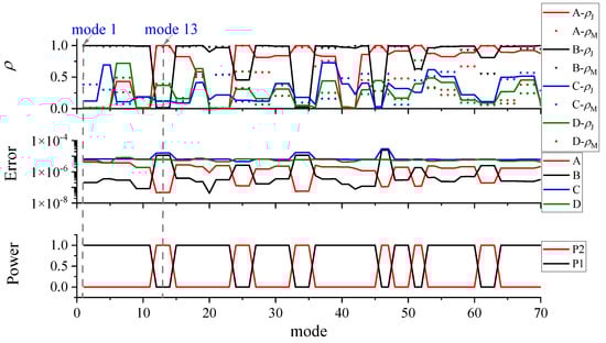
Figure 3. Boundary condition judgements of four problems for the first 70 lower-order modes by using correlation coefficient and error schemes. The resulting power is also plotted in the last graph.

Herein, we can select any one physical mode and spurious mode from Figure 2 and Figure 3 to demonstrate their current distributions. For convenience, modes 1 and 13 are considered, where mode 1 is the first spurious mode in Figure 2 and mode 13 is the first physical mode in Figure 2 for scattering problem (A). The corresponding characteristic electric and magnetic currents are displayed in Figure 4 and Figure 5, compared with the new ones from the boundary conditions (BCs) of the four cases. Symbols J and M represent known electric and magnetic currents obtained from Equation (19), while symbols J’(M) and M’(J) represent new currents by submitting M and J into one BC of the four problems. The prefixes A, B, C and D represent the BCs of problems (A), (B), (C), and (D). As previously mentioned, original currents should be matched with the resulting new currents if this mode satisfies a relevant BC. In Figure 4, it is apparently observed that the original currents (J, M) of mode 1 agree well with the new currents (B-J’(M), B-M’(J) from the BC of problem (B), which demonstrates mode 1 obeys the BC of problem (B). Similarly, mode 13 obeys the BC of problem (A), as displayed in Figure 5.

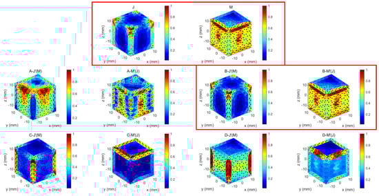
Figure 4. Comparison of characteristic electric and magnetic current distributions (J, M) of mode 1 (spurious mode) obtained from Equation (19) at 2.0 GHz, with other corresponding currents (J’(M), M’(J)) generated by submitting (M, J) into boundary conditions of problems (A), (B), (C) and (D).

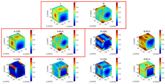
Figure 5. Comparison of characteristic electric and magnetic current distributions (J, M) of mode 13 (physical mode) obtained from Equation (19) at 2.0 GHz, with other corresponding currents (J’(M), M’(J)) generated by submitting (M, J) into boundary conditions of problems (A), (B), (C) and (D).

Furthermore, the modal powers of the first 70 lower-order modes are demonstrated in the bottom sub-figure of Figure 3. Here, ${\mathbb{P}}_2={\mathbb{F}}_n^H{\tilde{\mathbb{R}}}_2{\mathbb{F}}_n$ means the radiated power of the n-th mode for problem A or dissipated power for problem B, and ${\mathbb{P}}_1={\mathbb{F}}_n^H{\tilde{\mathbb{R}}}_1{\mathbb{F}}_n$ indicates the dissipated power of the n-th mode of problem (A) or radiated power of problem (B). We can find that the physical modes are modes with a unitary radiated power of problem (A), and the spurious modes are modes with zero radiated power of problem (A). Thus, these spurious modes are non-radiation modes for problem (A). However, the normalized radiated power of these modes are equal to one for problem (B).

The discussions above explain from the perspective of boundary conditions why the spurious modes are indeed solutions to problem (B), as found in [18], for lossless materials. However, the interesting phenomenon is that none of these modes satisfies the BCs of radiation problems (C) or (D). The characteristic modes are often considered to be source-free since GEE (19) does not contain an excitation source. Does this mean that the characteristic modes are appropriate for both scattering problems and radiation problems? Obviously, problems (A) and (C) are, respectively, the scattering and radiation problems. However, no one mode is found to satisfy the BC of problem (C). The characteristic modes of scattering problem (A) are not suitable for radiation problem (C). In other words, scattering systems and radiation systems are distinct. In a word, CH-PMCHWT-TCM indeed does not identify the boundary or object media for an external source scattering problem and also does not extract characteristic modes of an internal source radiation problem. The proper definitions are needed for the four cases.

3. Definition of Radiation Characteristic Modes

It is clear that the problems (A), (B), (C), and (D) are different with specific boundary conditions (15), (21), (23), and (25), although with the same PMCHWT Equation (17). Therefore, we understand that (i) the scattering problem (A) is to solve (17) subject to (15), (ii) the scattering problem (B) is to solve (17) subject to (21), (iii) the radiation problem (C) is to solve (17) subject to (23), and (iv) the radiation problem (D) is to solve (17) subject to (25).

In addition, our previous work [11,14] has addressed scattering problem (A) and proposed adequate formulations. The boundary condition is truly one of the key points. Another key point is the proper definition of the GEE, i.e., the right-hand side of the GEE should be related to radiation power [11,12,13]. These two points are taken into account in the following. Actually, we are chiefly concerned about scattering problem (A) and radiation problem (C) in engineering applications. Thus, we first derive the characteristic mode formulation of radiation problem (C) and then extend it to other problems.

For radiation problem (C), we substitute the solution of (17) to (23). Applying (29) to (17) and multiplying both sides by $\frac{1}{2}{\mathbb{F}}^H$, we obtain

$$\frac{1}{2}{\mathbb{J}}^H{\mathbb{Z}}_C\mathbb{J}=\frac{1}{2}{\mathbb{M}}^H{\mathbb{Y}}_C\mathbb{M}=\frac{1}{2}{\mathbb{F}}^H\mathbb{V}$$

(34)

in which

$${\mathbb{F}}^H=\left[\begin{array}{cc}{\mathbb{J}}^H& {\mathbb{M}}^H\end{array}\right]={\mathbb{J}}^H\left[\begin{array}{cc}\mathbb{I}& -{\eta }_1^{\ast }{({\mathbb{S}}_1^{+})}^H\end{array}\right]={\mathbb{M}}^H\left[\begin{array}{cc}{\zeta }_1^{\ast }{({\mathbb{S}}_1^{+})}^H& \mathbb{I}\end{array}\right]$$

(35)

$${\mathbb{Z}}_C=\left[\begin{array}{cc}\mathbb{I}& -{\eta }_2^{\ast }{({\mathbb{S}}_2^{-})}^H\end{array}\right]\tilde{\mathbb{Z}}\left[\begin{array}{c}\mathbb{I}\\ -{\eta }_2{\mathbb{S}}_2^{-}\end{array}\right]$$

(36)

$${\mathbb{Y}}_C=\left[\begin{array}{cc}{\zeta }_2^{\ast }{({\mathbb{S}}_2^{-})}^H& \mathbb{I}\end{array}\right]\tilde{\mathbb{Z}}\left[\begin{array}{c}{\zeta }_2{\mathbb{S}}_1^{-}\\ \mathbb{I}\end{array}\right]$$

(37)

and $\mathbb{I}$ is an identity matrix. It should be noted that (34) is the total power of the system.

In this paper, we adopt the GEE form as in [11,12,13], where the right-hand side of the equations should be related to radiated power in order to obtain the maximal radiation characteristic. Therefore, the GEE is defined by

$${\mathbb{Z}}_C{\mathbb{J}}_n=\left(1+j{\lambda }_n\right){\mathbb{R}}_C{\mathbb{J}}_n \mathrm{or} {\mathbb{Y}}_C{\mathbb{M}}_n=\left(1+j{\lambda }_n\right){\mathbb{G}}_C{\mathbb{M}}_n$$

(38)

with radiated power operators

$${\mathbb{R}}_C=\left[\begin{array}{cc}\mathbb{I}& -{\eta }_2^{\ast }{({\mathbb{S}}_2^{-})}^H\end{array}\right]{\tilde{\mathbb{R}}}_2\left[\begin{array}{c}\mathbb{I}\\ -{\eta }_2{\mathbb{S}}_2^{-}\end{array}\right]$$

(39)

$${\mathbb{G}}_C=\left[\begin{array}{cc}{\zeta }_2^{\ast }{({\mathbb{S}}_2^{-})}^H& \mathbb{I}\end{array}\right]{\tilde{\mathbb{R}}}_2\left[\begin{array}{c}{\zeta }_2{\mathbb{S}}_1^{-}\\ \mathbb{I}\end{array}\right]$$

(40)

which are proved in Appendix A.

Following the same process, GEEs for case (D) in Figure 1 can be given as

$${\mathbb{Z}}_D{\mathbb{J}}_n=\left(1+j{\lambda }_n\right){\mathbb{R}}_D{\mathbb{J}}_n \mathrm{or} {\mathbb{Y}}_D{\mathbb{M}}_n=\left(1+j{\lambda }_n\right){\mathbb{G}}_D{\mathbb{M}}_n.$$

(41)

with the following operators:

$${\mathbb{Z}}_D=\left[\begin{array}{cc}\mathbb{I}& -{\eta }_1^{\ast }{({\mathbb{S}}_1^{-})}^H\end{array}\right]\tilde{\mathbb{Z}}\left[\begin{array}{c}\mathbb{I}\\ -{\eta }_1{\mathbb{S}}_1^{-}\end{array}\right]$$

(42)

$${\mathbb{Y}}_D=\left[\begin{array}{cc}{\zeta }_1^{\ast }{({\mathbb{S}}_1^{-})}^H& \mathbb{I}\end{array}\right]\tilde{\mathbb{Z}}\left[\begin{array}{c}{\zeta }_1{\mathbb{S}}_1^{-}\\ \mathbb{I}\end{array}\right]$$

(43)

$${\mathbb{R}}_D=\left[\begin{array}{cc}\mathbb{I}& -{\eta }_1^{\ast }{({\mathbb{S}}_1^{-})}^H\end{array}\right]{\tilde{\mathbb{R}}}_1\left[\begin{array}{c}\mathbb{I}\\ -{\eta }_1{\mathbb{S}}_1^{-}\end{array}\right]$$

(44)

$${\mathbb{G}}_D=\left[\begin{array}{cc}{\zeta }_1^{\ast }{({\mathbb{S}}_1^{-})}^H& \mathbb{I}\end{array}\right]{\tilde{\mathbb{R}}}_1\left[\begin{array}{c}{\zeta }_1{\mathbb{S}}_1^{-}\\ \mathbb{I}\end{array}\right].$$

(45)

Alternatively, due to ${\mathbb{F}}^H{\tilde{\mathbb{Z}}}_2^{+}\mathbb{F}=0$ by (23), which would give $-\frac{1}{2}{\mathbb{F}}^H\mathbb{D}\mathbb{F}={\mathbb{F}}^H{\tilde{\mathbb{R}}}_2\mathbb{F}$ and ${\mathbb{F}}^H{\tilde{\mathbb{X}}}_2\mathbb{F}=0$, we may replace $\tilde{\mathbb{Z}}$ with ${\tilde{\mathbb{Z}}}_1+{\tilde{\mathbb{R}}}_2$ for problem (C). In the same way, we may replace $\tilde{\mathbb{Z}}$ with ${\tilde{\mathbb{Z}}}_2+{\tilde{\mathbb{R}}}_1$ for problem (D).

Similarly, GEEs for scattering problems (A) and (B) are shown as follows:

$${\mathbb{Z}}_A{\mathbb{J}}_n=\left(1+j{\lambda }_n\right){\mathbb{R}}_A{\mathbb{J}}_n \mathrm{or} {\mathbb{Y}}_A{\mathbb{M}}_n=\left(1+j{\lambda }_n\right){\mathbb{G}}_A{\mathbb{M}}_n,$$

(46)

$${\mathbb{Z}}_B{\mathbb{J}}_n=\left(1+j{\lambda }_n\right){\mathbb{R}}_B{\mathbb{J}}_n \mathrm{or} {\mathbb{Y}}_B{\mathbb{M}}_n=\left(1+j{\lambda }_n\right){\mathbb{G}}_B{\mathbb{M}}_n.$$

(47)

in which ${\mathbb{Z}}_A$, ${\mathbb{R}}_A$, ${\mathbb{Y}}_A$ and ${\mathbb{G}}_A$ can be obtained by replacing ${\mathbb{S}}_2^{-}$ in ${\mathbb{Z}}_C$, ${\mathbb{R}}_C$, ${\mathbb{Y}}_C$ and ${\mathbb{G}}_C$ with ${\mathbb{S}}_2^{+}$. Similarly, ${\mathbb{Z}}_B$, ${\mathbb{R}}_B$, ${\mathbb{Y}}_B$ and ${\mathbb{G}}_B$ can be obtained by replacing ${\mathbb{S}}_1^{-}$ in ${\mathbb{Z}}_D$, ${\mathbb{R}}_D$, ${\mathbb{Y}}_D$ and ${\mathbb{G}}_D$ with ${\mathbb{S}}_1^{+}$. Due to ${\mathbb{F}}^H{\tilde{\mathbb{Z}}}_1^{-}\mathbb{F}=0$, which would give $\frac{1}{2}{\mathbb{F}}^H\mathbb{D}\mathbb{F}={\mathbb{F}}^H{\tilde{\mathbb{R}}}_2\mathbb{F}$ and ${\mathbb{F}}^H{\tilde{\mathbb{X}}}_2\mathbb{F}=0$, we may replace $\tilde{\mathbb{Z}}$ with ${\tilde{\mathbb{Z}}}_1+\frac{1}{2}\mathbb{D}$ for problem (A). Likewise, we may replace $\tilde{\mathbb{Z}}$ with ${\tilde{\mathbb{Z}}}_2-\frac{1}{2}\mathbb{D}$ for problem (B). Specifically, we may replace $\tilde{\mathbb{Z}}$ with ${\tilde{\mathbb{Z}}}_1$ for problem (A) and with ${\tilde{\mathbb{Z}}}_2$ for problem (B) when the material is lossless.

4. Numerical Results

4.1. Cubic DR

We continue to consider the aforementioned cubic DR to compare scattering and radiation systems. The real parts of the characteristic eigenvalues of the first 150 lower-order modes are illustrated in Figure 6 using (46), (47), (38) and (41). In Figure 6a, the CMs of problem (A) and problem (B) are matched well with physical modes and spurious modes of CH-PMCHWT-TCM, as presented in Figure 2, just as in [18]. This also illustrates that spurious modes are solutions to problem (B) rather than problems (A), (C) and (D), for this case. The real parts of the characteristic modes of problem (A) are almost opposite to those of problem (B). The same phenomenon can be found for problem (C) with problem (D). The concerned resonant frequency points can be obtained from Figure 7, which shows the magnitudes of characteristic eigenvalues versus frequency range from 2.0 GHz to 4.5 GHz. In this frequency range, there are three, four, three and five resonant frequency points for problems (A), (B), (C), and (D), respectively, as listed in Table 1. Particularly, these four problems all have three frequency points close to 3.0 GHz, 4.0 GHz and 4.28 GHz, respectively. In order to figure out their relationships, we will demonstrate their currents and patterns in the following part.

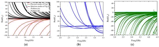
Figure 6. The real parts of characteristic eigenvalues with frequency range from 2.0 GHz to 4.5 GHz for four different problems. (a) Problems (A) and (B); (b) problem (C); (c) problem (D).

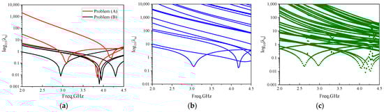
Figure 7. Magnitudes of characteristic eigenvalues in the frequency range from 2.0 GHz to 4.5 GHz for the four different problems. (a) Problems (A) and (B); (b) problem (C); (c) problem (D).

Table 1. Resonant Frequency (GHz) for Four Different Problems.

Mode	1	2	3	4	5	6
Problem (A)	--	3.08	--	3.88	--	4.18
Problem (B)	--	2.98	3.92	3.98	--	4.30
Problem (C)	--	3.05	--	4.18	--	4.35
Problem (D)	2.62	2.98	--	4.05	4.15	4.28

Firstly, the resonant modes near 3.0 GHz are denoted as ‘mode 2’. The resulting characteristic electric and magnetic currents are shown in Figure 8. We can see that the currents for the four problems are different. Nevertheless, the normalized scattering/radiation patterns of problems (A), (B), and (C) look similar, except their maximal scattering/radiation directions are different, as shown in Figure 9. However, the pattern of problem (D) is apparently different from the others. Two similar patterns do not mean that the two modes are the same, while two modes with the same currents must lead to the same patterns. References [10,11,12] have evaluated the characteristic modes of a cylindrical DR for problem (A), wherein there exist two different modes, i.e., TE₀₁ and TM₀₁, whose currents are different, but the patterns look similar. Therefore, we should judge whether the two modes are the same or not according to their characteristic electric and magnetic current distributions rather than their patterns. For other resonant modes near 4.0 GHz and 4.28 GHz, i.e., ‘mode 4’ and ‘mode 6’, the characteristic currents and patterns of the four problems are different, whose patterns are displayed in Figure 10 and Figure 11, respectively.

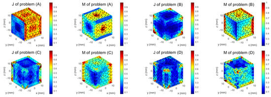
Figure 8. Characteristic electric and magnetic current distributions of mode 2 at 2.0 GHz, where the left column represents electric current and the right column represents magnetic current in every sub-figure.

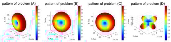
Figure 9. Normalized characteristic patterns of mode 2 for the four different problems at 2.0 GHz.

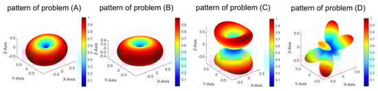
Figure 10. Normalized characteristic patterns of mode 4 for the four different problems at 2.0 GHz.

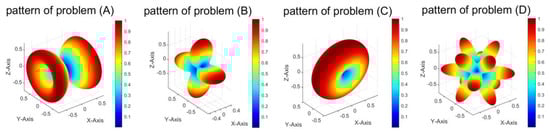
Figure 11. Normalized characteristic patterns of mode for the four different problems at 2.0 GHz.

In a word, the CMs of the four problems are different, even in spite of having several adjacent resonant frequency points. Actually, we have tested the remaining characteristic modes of the four problems and found that their currents are indeed different, which are not shown to save space.

4.2. Spherical DR

In Section 4.1, we have demonstrated that the CMs of scattering problems are distinct from those of radiation problems. Specifically, the spurious modes of CH-PMCHWT-TCM for a lossless medium are indeed solutions to problem (B), as reported in [18]. In other words, these modes are not solutions to problem (C) such that they could not be excited inside the object. Nevertheless, [17] excited one spurious mode for a two-dimensional infinity cylinder. To find this possibility, we need to choose a suitable object in order to find one mode, which is a solution to problem (B) and whose currents are very similar to problem (C), so that it may be excited approximately for problem (C). For this reason, we will consider a spherical symmetrical construct.

Thereupon, a spherical DR with a radius of 15.71 mm is considered in this subsection, whose material parameters are the same as the cubic DR. The real parts of the characteristic eigenvalues of the first 150 lower-order modes are shown in Figure 12 using (38), (41), (46) and (47). Specifically, the results for problems (A) and (B) agree well with those in [18], as plotted in Figure 12a. The resonant frequency points of four problems can be obtained by observing the magnitudes of characteristic eigenvalues, as displayed in Figure 13. There are three resonant frequency points for problem (C) and two for problem (D), which are listed in Table 2 compared with those of problems (A) and (B).

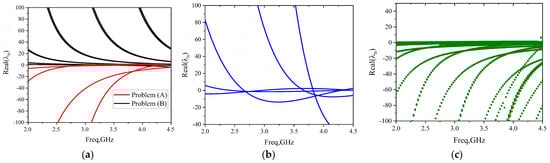
Figure 12. The real parts of characteristic eigenvalues of the first 150 lower-order modes in the frequency range from 2.0 GHz to 4.5 GHz for the four different problems. (a) Problems (A) and (B); (b) problem (C); (c) problem (D).

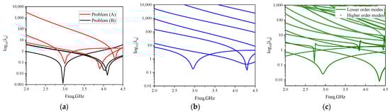
Figure 13. Magnitudes of characteristic eigenvalues of the first 150 lower-order modes in the frequency range from 2.0 GHz to 4.5 GHz for the four different problems. (a) Problems (A) and (B); (b) problem (C); (c) problem (D).

Table 2. Resonant Frequency (GHz) for Four Different Problems.

Mode	1	2	3
Problem (A)	2.96	3.88	4.27
Problem (B)	2.97	4.05	4.10
Problem (C)	2.95	4.28	4.30
Problem (D)	2.95	--	4.35

For this case, the first resonant frequencies are almost consistent, i.e., ‘mode 1’. The resulting characteristic electric and magnetic currents of problem (B) seem to be the dual ones of problem (A), as shown in Figure 14. Here, ‘dual’ means the electric current of mode 1 of problem (A) is similar to the magnetic current of mode 1 of problem (B), and vice versa. Additionally, the currents of problem (C) are almost the same as those of problem (A). The currents of problem (D) are completely different from the others. The resulting patterns of problems (A), (B), and (C) are nearly the same, which are different from the ones of problem (D), as presented in Figure 15. The orders of CMs of problem (D) are also higher than other problems. For the other resonant modes near 4.0 GHz, i.e., ‘mode 2’ and ‘mode 3’, the differences of the four problems will be increased. Specifically, the characteristic electric and magnetic currents of mode 3 resonating at 4.3 GHz for problem (C) look the same as those of mode 1 resonating at 2.97 GHz for problem (B), which must lead to a similar pattern, as shown in Figure 16.

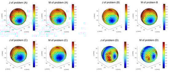
Figure 14. Characteristic electric and magnetic current distributions of the modes resonating near 2.95 GHz for the four different problems at 2.0 GHz, where the left column represents electric current and the right column represents magnetic current in every sub-figure.

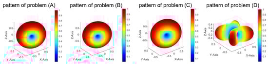
Figure 15. Normalized characteristic patterns of the modes resonant near 2.95 GHz for four different problems at 2.0 GHz.

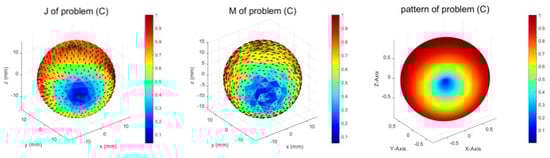
Figure 16. Characteristic current distributions and normalized pattern of mode 3 resonating near 4.3 GHz for problem (C) at 2.0 GHz, where the left column represents electric current, the middle column represents magnetic current, and the right column represents normalized pattern.

Therefore, there probably exists approximately the same mode for the scattering and radiation of a dielectric object only when the object is a special structure and at a special frequency. There also exists one mode of problem (B) that has almost the same currents as those of one mode of problem (C). On the one hand, this phenomenon may explain the possibility in [17]. It should be noted that this is just a special case. On the other hand, this also explains why some CMs extracted under the scattering framework may be approximately applicable to the analysis of some special radiation systems. Generally, the resonant modes are different for scattering and radiation problems for an arbitrary object.

5. Conclusions

In this paper, we investigate four physical problems and find the underlying reason why CH-PMCHWT-TCM is prone to generate spurious modes. The key point is that the impedance matrix of the PMCHWT equation cannot differentiate the two different media without the assistance of a dependent relationship between equivalent electric and magnetic currents or the boundary conditions. The conventional CMs are essentially constructed in the scattering framework. When they are applied to radiation problems, their dependent relationships are different, although they have the same impedance operator. In other words, the CMs in the scattering framework are not appropriate for a radiation system, and they are independent of a scattering excitation source rather than any excitation source. Then, we put forward new characteristic mode formulations for the two radiation problems. After numerical analysis, we find that the resonant modes of the four problems are essentially distinct in general. Nonetheless, there may exist some modes for which their resonant frequencies and characteristic electric and magnetic currents are similar for both the scattering and radiation problems in some special cases, such as a lossless spherically symmetric DR. This may explain why some CMs extracted under the scattering framework may be applicable to the analysis of some special radiation systems.

References

- Harrington, R.F.; Mautz, J.R. Theory of characteristic modes for conducting bodies. IEEE Trans. Antennas Propag. 1971, 19, 622–628. [Google Scholar] [CrossRef]
- Chen, Y.K.; Wang, C.F. Characteristic Modes: Theory and Applications in Antenna Engineering; Wiley Publishing: Hoboken, NJ, USA, 2015; p. 304. [Google Scholar]
- Shi, Y.; Meng, Z.K.; Wei, W.Y.; Zheng, W.; Li, L. Characteristic mode cancellation method and its application for antenna RCS reduction. IEEE Antennas Wirel. Propag. Lett. 2019, 18, 1784–1788. [Google Scholar] [CrossRef]
- Fritz-AnDRde, E.; Pérez-Miguel, A.; Gomez-Villanueva, R.; Jardon-Aguilar, H. Characteristic mode analysis applied to reduce the mutual coupling of a four-element patch MIMO antenna using a defected ground structure. IET Microw. Antennas Propag. 2019, 14, 215–226. [Google Scholar] [CrossRef]
- Harrington, R.F.; Mautz, J.R.; Chang, Y. Characteristic modes for dielectric and magnetic bodies. IEEE Trans. Antennas Propag. 1972, 20, 194–198. [Google Scholar] [CrossRef]
- Chang, Y.; Harrington, R.F. A surface formulation for characteristic modes of material bodies. IEEE Trans. Antennas Propag. 1977, 25, 789–795. [Google Scholar] [CrossRef]
- Alroughani, H.; Ethier, J.L.T.; McNamara, D.A. Observations on computational outcomes for the characteristic modes of dielectric objects. In Proceedings of the 2014 IEEE Antennas and Propagation Society International Symposium (APSURSI), Memphis, TN, USA, 6–11 July 2014; pp. 844–845. [Google Scholar]
- Chen, Y.K. Alternative surface integral equation-based characteristic mode analysis of dielectric resonator antennas. IET Microw. Antennas Propag. 2016, 10, 193–201. [Google Scholar] [CrossRef]
- Hu, F.G.; Wang, C.F. Integral equation formulations for characteristic modes of dielectric and magnetic bodies. IEEE Trans. Antennas Propag. 2016, 64, 4770–4776. [Google Scholar] [CrossRef]
- Lian, R.Z.; Pan, J.; Huang, S.D. Alternative surface integral equation formulations for characteristic modes of dielectric and magnetic bodies. IEEE Trans. Antennas Propag. 2017, 65, 4706–4716. [Google Scholar] [CrossRef]
- Guo, X.-Y.; Lian, R.-Z.; Zhang, H.-L.; Chan, C.-H.; Xia, M.-Y. Characteristic mode formulations for penetrable objects based on separation of dissipation power and use of single surface integral equation. IEEE Trans. Antennas Propag. 2021, 69, 1535–1544. [Google Scholar] [CrossRef]
- Ylä-Oijala, P.; Wallén, H.; Tzarouchis, D.C.; Sihvola, A. Surface integral equation-based characteristic mode formulation for penetrable bodies. IEEE Trans. Antennas Propag. 2018, 66, 3532–3539. [Google Scholar] [CrossRef]
- Ylä-Oijala, P. Generalized theory of characteristic modes. IEEE Trans. Antennas Propag. 2019, 67, 3915–3923. [Google Scholar] [CrossRef]
- Guo, X.-Y.; Lian, R.-Z.; Xia, M.-Y. Variant characteristic mode equations using different power operators for material bodies. IEEE Access 2021, 9, 62021–62028. [Google Scholar] [CrossRef]
- Miers, Z.T.; Lau, B.K. Computational analysis and verifications of characteristic modes in real materials. IEEE Trans. Antennas Propag. 2016, 64, 2595–2607. [Google Scholar] [CrossRef]
- Huang, S.; Pan, J.; Luo, Y. Investigations of non-physical characteristic modes of material bodies. IEEE Access 2018, 6, 17198–17204. [Google Scholar] [CrossRef]
- Bernabeu-Jiménez, T.; Valero-Nogueira, A.; Vico-Bondia, F.; Kishk, A.A. On the contribution to the field of the nonphysical characteristic modes in infinite dielectric circular cylinders under normal excitation. IEEE Trans. Antennas Propag. 2018, 66, 505–510. [Google Scholar] [CrossRef]
- Ylä-Oijala, P.; Wallén, H. PMCHWT-Based characteristic mode formulations for material bodies. IEEE Trans. Antennas Propag. 2020, 68, 2158–2165. [Google Scholar] [CrossRef]
- Lian, R.-Z.; Guo, X.-Y.; Xia, M.-Y. Entire-structure-oriented work-energy theorem (ES-WET)-based characteristic mode theory for material scattering objects. IEEE Trans. Antennas Propag. 2022, 70, 5699–5714. [Google Scholar] [CrossRef]
- Chen, Y.; Guo, L.; Yang, S. Mixed-potential integral equation based characteristic mode analysis of microstrip antennas. Inter. J. Antennas Propag. 2016, 2016, 1–8. [Google Scholar] [CrossRef]
- Lin, F.H.; Chen, Z.N. Low-profile wideband metasurface antennas using characteristic mode analysis. IEEE Trans. Antennas Propag. 2017, 65, 1706–1713. [Google Scholar] [CrossRef]
- Wu, Q. General metallic-dielectric structures: A characteristic mode analysis using volume-surface formulations. IEEE Antennas Propag. Mag. 2019, 61, 27–36. [Google Scholar] [CrossRef]
- Guan, L.; He, Z.; Ding, D.; Chen, R. Efficient characteristic mode analysis for radiation problems of antenna arrays. IEEE Trans. Antennas Propag. 2019, 67, 199–206. [Google Scholar] [CrossRef]
- Ylä-Oijala, P.; Taskinen, M. Calculation of CFIE impedance matrix elements with RWG and n/spl times/RWG functions. IEEE Trans. Antennas Propag. 2003, 51, 1837–1846. [Google Scholar] [CrossRef]
Disclaimer/Publisher’s Note: The statements, opinions and data contained in all publications are solely those of the individual author(s) and contributor(s) and not of MDPI and/or the editor(s). MDPI and/or the editor(s) disclaim responsibility for any injury to people or property resulting from any ideas, methods, instructions or products referred to in the content. |
© 2023 by the authors. Licensee MDPI, Basel, Switzerland. This article is an open access article distributed under the terms and conditions of the Creative Commons Attribution (CC BY) license (https://creativecommons.org/licenses/by/4.0/).