Abstract
In the Mallat algorithm, calculations are performed in the time domain. To speed up the signal conversion at each level, the wavelet coefficients are sequentially halved. This paper presents an algorithm for increasing the speed of multiscale signal analysis using fast Fourier transform. In this algorithm, calculations are performed in the frequency domain, which is why the authors call this algorithm multiscale analysis in the frequency domain. For each level of decomposition, the wavelet coefficients are determined from the signal and can be calculated in parallel, which reduces the conversion time. In addition, the zoom factor can be less than two. The Mallat algorithm uses non-symmetric wavelets, and to increase the accuracy of the reconstruction, large-order wavelets are obtained, which increases the transformation time. On the contrary, in our algorithm, depending on the sample length, the wavelets are symmetric and the time of the inverse wavelet transform can be faster by 6–7 orders of magnitude compared to the direct numerical calculation of the convolution. At the same time, the quality of analysis and the accuracy of signal reconstruction increase because the wavelet transform is strictly orthogonal.
1. Introduction
Using fast Fourier transform (FFT), it is possible to develop fast algorithms for continuous wavelet transform (WT). Using these algorithms, it is possible to develop a method of multiple-scale signal analysis (MSA) in the frequency domain that is different from the one developed earlier. Presently, for MSA signals, the Mallat algorithm [1] is used, which calculates the discrete wavelet transform faster due to the decimation of the wavelet coefficients. MSA is an -step discrete WT.
The Mallat algorithm has some drawbacks:
1. The scaling function needs to be designed.
2. The multiplicity of the analysis is fixed and cannot be changed.
3. It is impossible to get antisymmetric or symmetric wavelets.
4. The amplitude–frequency characteristics of the wavelets are uneven.
5. The sample length decreases by a factor of two for subsequent decomposition levels. As a result, the transition characteristic becomes flatter.
6. Only decomposition separable by rows and columns is used.
7. Large-order wavelets take a long time to compute.
To address these shortcomings, it is important to use MSA in the frequency domain. The advantage of the algorithm in the frequency domain is in the method of calculation. In the Mallat algorithm, it is impossible to calculate the wavelet coefficients in parallel [2], but in the frequency domain, it is possible. At the hardware level, to reduce the MSA time, this can be implemented by connecting FFT devices in parallel. For example, if the signal is decomposed into 10 levels (10 FFT devices), then with parallel computing, the calculation speed increases by 10 times. Field programmable gate array (FPGA) is well suited for solving this problem. To calculate the MSA in the frequency domain, the formula of continuous WT signals is used:
For data analysis, fast wavelet transform (FWT) is widely used. In [3], the authors introduced an open-source algorithm to calculate the past continuous wavelet transform (fCWT). The parallel environment of fCWT separated scale-independent and scale-dependent operations, while using optimized FFT that exploited downsampled wavelets. fCWT was shown to have the accuracy of CWT, to have 100 times higher spectral resolution than algorithms equal in speed, and to be 122 times and 34 times faster, respectively, than the reference and the fastest state-of-the-art implementations. The authors [3] also demonstrated its real-time performance, as confirmed by the real-time analysis ratio. According to the authors [3], fCWT provides an improved balance between speed and accuracy, which enables real-time, wide-band, high-quality, time–frequency analysis of non-stationary noisy signals. In [4], the authors proposed a multispectral image compression and encryption algorithm that combines chaos, WT, and KL transform for solving the security problem of multispectral image compression and transmission. In [5], a wavelet genetic (WAVEGEN) algorithm was developed to edit fatigue loading spectra using wavelet analysis. In this process, an optimization protocol using a genetic algorithm was included to automatically select the best wavelet editing parameters. In [6], the authors developed a novel shift variance theorem of the FWT suitable for the multiresolution analysis of streaming univariate datasets, using compactly supported Daubechies wavelets. The theorem was used to reduce the computational complexity of FWT and also to drastically reduce the number of wavelet coefficients to be estimated in forecasting the discrete WT one step ahead. For this reason, in [6], any FWT performed using the found shift variance properties was named reduced FWT. In [7], a wavelet-based dynamic-state feedback control strategy was proposed. The feedback gains were obtained through a linear quadratic regulator formulation, with cost weights adjusted according to suitable performance metrics. In [8], the authors proposed a new method based on a B-spline expansion of both the signal and the analysis wavelet and that allowed CWT computation at arbitrary scales. Its complexity was , where represents the size of the input signal; in other words, the cost is independent of the scale factor. A fast, continuous WT was developed in [9] for use with continuous mother wavelets and sampled datasets. The method differs in that, in [9], the wavelet was sampled in the frequency domain. In [10], the frequency response of the presented wavelets was uneven. In other words, for high and low frequencies, the gain differed by 2–3 times. With such a difference, it is impossible to reconstruct the signal or to perform a multiple-scale analysis of the signal. In [11], the authors presented the possibility of estimating surface roughness with computer vision using a wavelet transform in the frequency domain.
It takes a lot of time to calculate continuous WT by direct numerical integration for large amounts of information. Even when modern computers with a frequency of several GHz are used, it takes hundreds of seconds to decompose an image 512 × 512 pixels in size. Considering that it is necessary to produce WT for three colors, a crucial point is the implementation of fast algorithms for converting and reconstructing signals. Therefore, the numerical calculation of a continuous WT is performed in the frequency domain. The numerical calculation in the frequency domain is studied in articles [12,13,14,15,16]. In [12], the authors considered methods for constructing orthogonal wavelets in the frequency domain and synthesizing digital filters with a straight-angle frequency response by the method of constructing wavelets. The FFT, the Proni transform, and the wavelet transform were considered in [13]. The authors [13] considered forward and reverse WT algorithms, as well as their application for processing one-dimensional and two-dimensional signals. In [14], the application of orthogonal wavelets for image processing was considered. In [15], WT was considered in the Excel environment using the VBA programming language. Methods of constructing orthogonal wavelets and their application for image filtering were considered in [16]. The article suggested methods for the multiscale analysis of signals not in the time domain (unlike the Mallat algorithm), which allow image decomposition, reconstruction, and filtering. The design of wavelets with a rectangular frequency response (FR) in the frequency domain allows one to reduce the time of continuous WT by several orders of magnitude and to increase the resolution of the wavelets and the accuracy of the analysis.
2. Mallat Algorithm
In his algorithm, Mallat [2] used the ideas of subband (pyramidal) encoding of the speech signal, which is equivalent to passing a signal through high-pass and low-pass filters (HP and LP filters), for example, quadrature mirror filters. The simplest way of WP is to use the simplest scaling function and the Haar wavelet, when the quadrature mirror filter is obtained by summing and the difference of neighboring signal samples. Summation is equivalent to passing through an LP filter, and the difference is an HP filter. More complex wavelets, such as the th-order Daubechies wavelets, are used to calculate weighted sums and weighted differences; that is, the convolution of the signal with the impulse response of HP and LP filters, and detailed coefficients and approximation coefficients are obtained after the decimation of each second sample. Due to decimation, the number of counts decreases. As per the theory of digital filters, the smaller the number of samples, the wider the transient response of filters. After the first decomposition, all calculations are performed with detailing coefficients and approximation coefficients iteratively. The inverse WT is calculated in reverse order with coefficient interpolation.
To construct large-order wavelets, it is necessary to spend more time, although such wavelets are more symmetrical and thus the signal is reconstructed more accurately later. The decomposition of the signal for a discrete WT is performed according to the following formula:
where denotes the wavelet, is the scaling function, and are detailing and approximating coefficients, respectively.
As a result of the conversion, the signal is decomposed into different frequency domains, schematically shown in Figure 1. With an increase in the scale factor, each region is two times narrower than the previous frequency domain. Since the FRs of the filters are not rectangular, the spectra overlap.
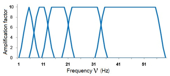
Figure 1.
Frequency domains of wavelets.
3. Calculation of Direct Continuous WT Signals Using FFT
Continuous WT is better than discrete WT, but direct convolution calculation sequences of continuous WT sequences according to Formula (1) take a long time. Direct numerical calculation of WT requires multiplication operations. In mathematics, the designation is accepted. To increase the speed, in this paper, we developed algorithms for direct continuous fast WT in the frequency domain using FFT. The number of computing operations of WT using FFT grows proportionally to . Using the harmonics of the signal and the wavelet, instead of calculating the convolution directly, we calculated the product of harmonics and obtained the wavelet spectrum by inverse Fourier transform. Such a transition to the frequency domain makes it possible to considerably increase the time of the wavelet transform. To obtain the wavelet spectrum of the signal by inverse Fourier transform of the complex conjugate spectra, the Fourier harmonics of the signal and the wavelet must be identified and multiplied.
The steps for the decomposition of the signal according to Formula (1) using the FFT are as follows:
1. Determine the harmonics of the signal :
2. Determine the harmonics of the wavelet :
3. Multiply the harmonics:
If the wavelets are even, then and
If the wavelets are odd, then and
The wavelet spectrum is determined by the formula
4. The Principle and Method of Signal Reconstruction Using FFT
The inverse continuous WT:
where is the normalizing coefficient and where is the Fourier spectrum of the basis function, stands for the cyclic frequency, and parameter indicates the degree of the scale multiplier.
Finding the convolution of the inverse WT by direct integration is inefficient. Therefore, in this paper, we developed a method for the inverse continuous fast WT in the frequency domain using FFT. The coefficient is calculated using Parseval’s theorem:
In practice, it is easier to calculate by comparing the maxima of the original and reconstructed signals. The coefficient is substituted into the formula:
Formulas (14) and (15) are used to calculate the inverse WT.
The following is the method for signal reconstruction according to Formula (15) using the FFT:
1. Calculate the harmonics of the :
2. Calculate the harmonics of the :
3. Calculate the harmonics of the of wavelet :
4. Calculate the harmonics of the of wavelet :
5. Multiply the harmonics:
For even wavelets, the series is made up of some cosines, and for odd ones, it consists of some sines. For even wavelets, and
For odd wavelets, and
6. Calculate the function for an even wavelet. As per Formula (22), Formula (23) is the function for an even wavelet:
7. Calculate the function for an odd wavelet. As per Formula (24), Formula (25) is the function for an odd wavelet:
In this formula, the symbol does not mean differentiation. In Formulas (26) and (27), and are different because of Formulas (22)–(25).
8. Determine coefficient C using Formula (14).
9. Determine S(n) according to the formula
In Formula (28), all levels of are summed up.
5. Using the Developed Methods of Forward and Inverse WT for MSA
In MSA using discrete WT, the Hilbert space is represented as a sequence of nested closed subspaces . Many references, for example, [17,18,19,20,21], describe the use of MSA on discrete WT. The union of these subspaces form a space . Subspaces are nested .
In the case of multiscale analysis of signals using the forward and inverse WT methods, we use levels ranging from to sequentially. We first use the level; then the sum of and levels; then the sum of , , and levels; and so on. Unlike discrete WT, the numbering of subspaces is reversed. Subspaces are nested in reverse:
is the union of subspaces. As m decreases, the subspaces expand. At the maximum value of , the signal is roughly approximated. The depth of decomposition (decomposition) of the signal is called the maximum value of . The accuracy of the approximation increases with decreasing values of The signal can be represented as a set of successive approximations. We obtain the functions .
These functions can be easily obtained programmatically. Table 1 presents a listing of the program for MSA in Visual Basic for Applications (VBA).

Table 1.
Listing of the program for MSA in VBA.
In the program, summation starts from to , i.e., levels are used. Even in Formula (28), levels are used, but indexing starts from and ends with the number . In the program, plays the role of and plays the role of . It is also possible to say that .
Figure 2 shows some of the functions of .
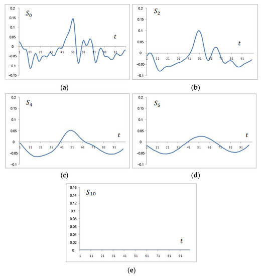
Figure 2.
Multiple-scale analysis of the function: (a) the signal obtained by adding all the decomposition levels, (b) the approximation of the signal obtained by adding 10-2 levels, (c) the approximation of the signal obtained by adding 10-4 levels, (d) the approximation of the signal obtained by adding 10-5 levels, and (e) the roughest approximation of the signal obtained by adding only 10 levels.
Figure 2 shows that the more the functions with a lower value of , the more accurate the approximation. For the original signal with the reconstructed signal, the Pearson correlation coefficient is 0.9992 when constructing wavelets based on Gaussian functions. In this case, the number of counts is 1024. As the number of counts decreases, the correlation coefficient decreases slightly because the uneven frequency response is more affected, as shown in Figure 1.
If for the Mallat algorithm, the MSA of signals can be performed with a coefficient of variation of the scale factor of 2 degrees of an integer , then for the developed algorithms in the frequency domain, the multiplicity of analysis can be less than 2.
To investigate the fine details of the signal, it is possible to plot the function or their sums in reverse order. By adopting the designation , , etc., it is possible to consider these graphs. Figure 3 shows approximately a tenth of the function.
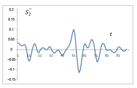
Figure 3.
Summation in reverse order.
We obtained the MSA of images similarly. To do this, all pixels of three colors were read from the image by progressive horizontal and vertical scanning; that is, the image was converted into a one-dimensional signal. Each color was decomposed into different levels. After that, the signal was converted back from one-dimensional to two-dimensional. Then, the pixels of the horizontal scan were added to the pixels of the vertical scan for each level and color. That is, a pixel with coordinates of the horizontal sweep was folded with a pixel with coordinates of the vertical sweep, a pixel with coordinates of the horizontal sweep was folded with a pixel with coordinates , and so on.
6. Construction of Wavelets in the Frequency Domain
According to the authors of [22], it is impossible to reconstruct the signal using continuous WT and the transformation is non-orthogonal. However, in this study, after numerous studies, we managed to construct orthogonal antisymmetric and symmetric wavelets in the frequency domain. We also managed to reduce the conversion time compared to the Mallat algorithm and reconstruct the signal more accurately than in the time domain. Some researchers have presented orthogonal polynomials with high-energy compaction, for example, in [23]. The FR of these polynomials is similar to that of wavelets based on Gauss functions. However, in this study, we worked with wavelets with a rectangular FR.
The theory of digital filters and the construction of wavelets are presented from different points of view. In the frequency domain, there is no difference between the pulse characteristics of filters and wavelets. Low-pass filters are equivalent to wavelets with the largest scale factor, bandpass filters are equivalent to wavelets with an average scale factor, and high-pass filters are equivalent to wavelets with the smallest scale factor. The synthesis of digital filters with a rectangular FR and a linear-phase response is arguably the same as the construction of orthogonal antisymmetric and symmetric wavelets. The theory of digital filters based on the Paley–Wiener criterion proves that it is not possible to obtain filters with a rectangular FR. In addition, a rectangular FR leads to the Gibbs phenomenon. However, in this study, we found that it is possible to avoid the Gibbs phenomenon and obtain filters and wavelets with a rectangular FR.
For accurate reconstruction of the signal, the frequency regions (spectra) of the wavelets should not overlap each other, as shown in Figure 1. They should be positioned as in Figure 4. This arrangement of the spectra indicates that the wavelets are strictly orthogonal.
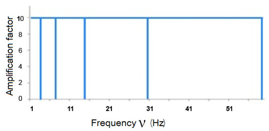
Figure 4.
Frequency domains of strictly orthogonal wavelets.
The scientific literature on WT states that discrete wavelets are orthogonal, which is not quite true because the frequency characteristics of all such wavelets overlap (Figure 1). We can say that all wavelets designed for discrete WT are not strictly orthogonal. This and a nonlinear frequency response distort the reconstructed signal. Using the method of calculating continuous WT in the time domain, it is possible to produce MSA with a multiplicity of less than two, which allows us to increase the number of decomposition levels and examine the signal in more detail. During the research, strictly orthogonal symmetric and antisymmetric wavelets were constructed. The frequency characteristics did not overlap (Figure 4). Studies show that the smaller the overlap, the smaller the scalar product of wavelets with different scale coefficients. If the scalar product tends to zero, then the wavelets are more orthogonal.
7. Ways to Increase the Speed of Continuous WT
To reduce the calculation time, it is necessary to make some changes in the algorithms of forward and inverse WT in the frequency domain.
The first way is to obtain wavelets in the frequency domain so as not to find harmonics , by the second stage.
The second way is to use the parity or odd property of wavelets, that is, symmetry and antisymmetry. For even wavelets, harmonics are made up of some cosines, and for odd ones, they are made up of some sines.
The third way is to calculate the inverse Fourier transforms from the complex conjugate spectrum for small-scale coefficients through a smaller interval and for large-scale coefficients through a larger interval. Table 2 presents the listing of the program in VBA.
Table 2.
Listing of the program in VBA.
The fourth method is to calculate the wavelet spectrum for one color, since the wavelet coefficients of the three primary colors of the additive RGB model have the same value. This can be used for compression because for small wavelet coefficients, threefold compression is obtained without encoding. In the human eye, 130 million rods are responsible for twilight vision and 7 million cones are responsible for color vision. Since colors appear only at large scales, the cones are located farther apart than the rods and the intensity of the wavelet coefficients for small-scale coefficients is less than that for large ones, which means that the radiation sources should be more sensitive for small scales. The sensitivity of the rods should be higher than that of the cones. Indeed, the rods sense a weaker light than the cones.
The fifth method is to calculate wavelets in the frequency domain, which excludes the defining of the normalizing coefficient.
The sixth way is to use the fourth way in reconstruction so that the wavelet coefficients of the same color can be used for all colors in the inverse WT algorithm and multiscale signal analysis.
The seventh way is to not calculate the Fourier transform for the largest-scale factor since it is enough to calculate the average value of the signal.
The eighth way is to obtain wavelets so that it is possible to reconstruct the signal with the order of computational operations . Thus, to sample a signal from 32,768 samples, it is possible to reduce the signal reconstruction time by 1000 times compared with the algorithm using FFT. The reconstruction time compared to the direct numerical integration of convolution is more than 10,000,000 times. In this study, the results of the WT signals were compared for direct calculation and calculation using FFT. The calculation time by direct numerical integration and the calculation of WT using FFT were compared in Visual C++. To measure small intervals in Visual C++, a real-time tag counter was used, access to which was implemented using the RDTSC (ReaD from Time Stamp Counter) assembly command. The TSC (Time Stamp Counter) is a 64-bit register whose contents are incremented with each clock cycle of the processor core. Each time, a hardware reset (RESET signal) starts counting in the TSC counter from zero. The bit depth of the register provides a countdown without overflow for hundreds of years. The processor clock frequency determines the resolution of the counter. The minimum time interval between two measurements is equal to the inverse value of the clock frequency. For a used processor with a clock frequency of 2.54 GHz, the resolution is 0.39 ns. The clock frequency is determined using a real-time TSC counter. The RDTSC command returns the number of clock cycles since the processor was started, placing the result in a pair of general-purpose registers EDX:EAX. To measure the calculation time of the WT, a program was written using the built-in C++ assembler. The counter was graded using the standard OS function Sleep. The Sleep function suspends the execution of the stream for 1000 ms if the function parameter is 1000. The TSC counter readings are read before calling the Sleep function and after returning from it. The difference of these readings is stored in the t_time variable. The number of machine clock cycles that have passed in 1 s of t_time are divided by 1,000,000 and stored in the n_count coefficient, which determines the number of clock cycles in 1 microsecond. Since the t_time variable is not zero even in the absence of the Sleep function, it is necessary to make corrections to the t_time variable. After calculating the calibration coefficient n_count, the WT is profiled as follows: The TSC counter readings are read before calculating the WT. After the conversion is completed, they are stored in the t_time variable. The resulting t_time value is divided by the calibration coefficient n_count and stored in a variable that shows the execution time of the WT in microseconds.
Such an increase in the calculation speed of WT can be explained by the fact that when calculating in the frequency domain, the computed wavelets are not only strictly orthogonal but also normalized, that is, orthonormalized. In addition, the wavelets have a rectangular FR, which cannot be obtained in the time domain due to the Gibbs phenomenon. Figure 5 shows one of the waveforms constructed in the frequency domain. Figure 6 shows the FR of this wavelet in decibels. In the case of a delay, the attenuation is about −300 dB. It can be argued that such wavelets are strictly orthogonal. Figure 7 shows the FR of this wavelet. There are no ripples in the bandwidth on the FR, no transition strip, and no Gibbs phenomenon. Figure 8 shows the FR of high-frequency filters synthesized in the time and frequency domains (in dB). The FR of a filter synthesized in the time domain is represented up to a frequency of 128 units, and the FR of a filter not synthesized in the time domain is represented from 129 to 256. In Figure 8, it is possible to see how the FR of the filters is considerably different.
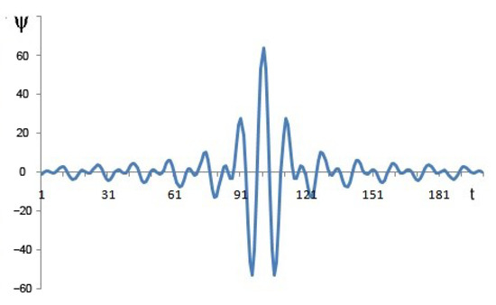
Figure 5.
Orthogonal symmetric wavelet.
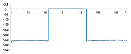
Figure 6.
Frequency response in dB.
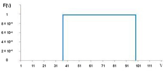
Figure 7.
Frequency response.
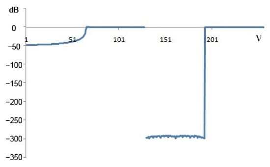
Figure 8.
Frequency response in dB.
The parameters of the impulse response of the filter are determined as follows:
Several examples for multiscale image analysis and image reconstructions can be found in [13].
8. Conclusions
When using wavelets based on derivatives of the Gaussian function, for the original signal with the reconstructed signal, the Pearson correlation coefficient is 0.9992. Wavelets or digital filters that are not obtained in the time domain have a rectangular FR, and there is no Gibbs phenomenon. Such wavelets make it possible to accurately restore the signal, and the Pearson correlation coefficient for such wavelets is 0.99999998. The calculation time of the inverse WT signal with a sample size of 262,144 samples decreased by 5000 times compared to the algorithm using FFT and by at least 10,000,000 times compared to direct numerical integration. Images with a size of 512 × 512 pixels are reconstructed in milliseconds. Thus, the algorithm can be implemented in near-real time.
Author Contributions
Conceptualization, V.Ď.; data curation, S.G.C.; formal analysis, S.G.C.; investigation, V.I.S.; methodology, V.Ď.; resources, V.I.S.; supervision, V.Ď.; validation, S.G.C.; visualization, V.I.S. All authors have read and agreed to the published version of the manuscript.
Funding
This study received no external funding.
Conflicts of Interest
The authors declare no conflict of interest.
Notation
| The step of discrete WT | |
| Wavelet spectrum | |
| The signal for decomposition | |
| The wavelet shifted by b by the scale factor a | |
| The wavelet for discrete wavelet transform | |
| Scaling function | |
| Detailing and approximating coefficients | |
| N | The number of multiplication operations |
| The harmonics of the signal | |
| Digitized signal | |
| The harmonics of the wavelet | |
| The indicator of the degree of the scale multiplier | |
| Normalizing coefficient | |
| Fourier spectrum of the basis function | |
| The harmonics of the | |
| Digitized signal | |
| Inverse transformation of the m-th level | |
| Hilbert space | |
| Hilbert subspaces | |
| Reverse signal approximation |
References
- Mallat, S.G. A theory for multiresolution signal decomposition: The wavelet representation. IEEE Trans. Pattern Anal. Mach. Intell. 1989, 11, 674–693. [Google Scholar] [CrossRef]
- Mallat, S.G. A Wavelet Tour of Signal Processing; Academic Press: San Diego, CA, USA, 1999; ISBN 978-0-12-466606-1. [Google Scholar]
- Arts, L.P.A.; Van den Broek, E.L. The fast continuous wavelet transformation (fCWT) for real-time, high-quality, noise-resistant time–frequency analysis. Nat. Comput. Sci. 2022, 2, 47–58. [Google Scholar] [CrossRef]
- Xu, D.-D.; Yu, X.; Du, L.-M.; Bi, G.-L. Multispectral image compression and encryption algorithm based on chaos and fast wavelet transform. Spectrosc. Spectr. Anal. 2022, 42, 2976–2982. [Google Scholar] [CrossRef]
- Mohseni, M.; Santhanam, S.; Williams, J.; Thakker, A.; Nataraj, C. Systematic fatigue spectrum editing by fast wavelet transform and genetic algorithm. Fatigue Fract. Eng. Mater. Struct. 2022, 45, 69–83. [Google Scholar] [CrossRef]
- Stocchi, M.; Marchesi, M. Fast wavelet transform assisted predictors of streaming time series. SoftwareX 2018, 8, 1–4. [Google Scholar] [CrossRef]
- Uzinski, J.C.; Paiva, H.M.; Galvão, R.K.H.; Assunção, E.; Duarte, M.A.Q.; Villarreal, F. A dynamic-state feedback approach employing a new state-space description for the fast wavelet transform with multiple decomposition levels. J. Control. Autom. Electr. Syst. 2017, 28, 303–313. [Google Scholar] [CrossRef]
- Muñoz, A.; Ertlé, R.; Unser, M. Fast continuous wavelet transform based on B-splines. Proc. SPIE Int. Soc. Opt. Eng. 2001, 4478, 224–229. [Google Scholar] [CrossRef]
- Dress, W.B. Applications of a fast continuous wavelet transform. Proc. SPIE Int. Soc. Opt. Eng. 1997, 3078, 570–580. [Google Scholar] [CrossRef]
- Bayram, I.; Selesnick, I.W. Frequency-Domain Design of Overcomplete Rational-Dilation Wavelet Transforms. IEEE Trans. Signal Process. 2009, 57, 2957–2972. [Google Scholar] [CrossRef]
- Morala-Argüello, P.; Barreiro, J.; Alegre, E. A Evaluation of Surface Roughness Classes by Computer Vision Using Wavelet Transform in the Frequency Domain. Int. J. Adv. Manuf. Technol. 2011, 59, 213–220. [Google Scholar] [CrossRef]
- Ďuriš, V.; Semenov, V.I.; Chumarov, S.G. Wavelets and digital filters designed and synthesized in the time and frequency domains. Math. Biosci. Eng. 2022, 19, 3056–3068. [Google Scholar] [CrossRef] [PubMed]
- Ďuriš, V.; Semenov, V.I.; Chumarov, S.G. Application of Continuous Fast Wavelet Transform for Signal Processing, 1st ed.; Sciemcee Publishing: London, UK, 2021; 181p, ISBN 978-1-9993071-9-6. [Google Scholar]
- Ďuriš, V.; Chumarov, S.G.; Mikheev, G.M.; Mikheev, K.G.; Semenov, V.I. The Orthogonal Wavelets in the Frequency Domain Used for the Images Filtering. IEEE Access 2020, 8, 211125–211134. [Google Scholar] [CrossRef]
- Ďuriš, V.; Semenov, V.I.; Chumarov, S.G. Wavelet Transform of Signals with VBA Applications, 1st ed.; Ste-Con: Karlsruhe, Germany, 2022; 203p, ISBN 978-3-945862-44-5. [Google Scholar]
- Semenov, V.I.; Mikheev, K.G.; Shurbin, A.K.; Mikheev, G.M. Construction of orthogonal wavelets in the frequency region for a multiscale signal analysis. Khim. Fiz. Mezoskopiya 2018, 20, 230–238. [Google Scholar]
- Meglic, A.; Goic, R. Wavelet multi-scale analysis of wind turbines smoothing effect and power fluctuations. In Proceedings of the 2021 9th International Renewable and Sustainable Energy Conference, IRSEC, Tetouan, Morocco, 23–27 November 2021. [Google Scholar] [CrossRef]
- Cheng, M.; Li, Q.; Lv, J.; Liu, W.; Wang, J. Multi-scale LSTM model for BGP anomaly classification. IEEE Trans. Serv. Comput. 2021, 14, 765–778. [Google Scholar] [CrossRef]
- Savari, C.; Li, K.; Barigou, M. Multiscale wavelet analysis of 3D lagrangian trajectories in a mechanically agitated vessel. Chem. Eng. Sci. 2022, 260, 117844. [Google Scholar] [CrossRef]
- Bales, S. Sovereign and bank dependence in the eurozone: A multi-scale approach using wavelet-network analysis. Int. Rev. Financ. Anal. 2022, 83, 102297. [Google Scholar] [CrossRef]
- Li, C.; Yang, X. An image encryption algorithm based on discrete fractional wavelet transform and quantum chaos. Optik 2022, 260, 169042. [Google Scholar] [CrossRef]
- Shumarova, O.; Ignat, S. Optimal choice of the type of wavelet for processing a signal from an eddy current sensor. Vestnik SGTU 2013, 4, 128–132. [Google Scholar]
- Abdulhussain, S.H.; Ramli, A.R.; Al-Haddad, S.A.R.; Mahmmod, B.M.; Jassim, W.A. On Computational Aspects of Tchebichef Polynomials for Higher Polynomial Order. IEEE Access 2017, 5, 2470–2478. [Google Scholar] [CrossRef]


Disclaimer/Publisher’s Note: The statements, opinions and data contained in all publications are solely those of the individual author(s) and contributor(s) and not of MDPI and/or the editor(s). MDPI and/or the editor(s) disclaim responsibility for any injury to people or property resulting from any ideas, methods, instructions or products referred to in the content. |
© 2023 by the authors. Licensee MDPI, Basel, Switzerland. This article is an open access article distributed under the terms and conditions of the Creative Commons Attribution (CC BY) license (https://creativecommons.org/licenses/by/4.0/).