Abstract
Resting-state functional connectivity has been widely used for the past few years to forecast Alzheimer’s disease (AD). However, the conventional correlation calculation does not consider different frequency band features that may hold the brain atrophies’ original functional connectivity relationships. Previous works focuses on low-order neurodynamics and precisely manipulates the mono-band frequency span of resting-state functional magnetic imaging (rs-fMRI). They specifically use the mono-band frequency span of rs-fMRI, leaving out the high-order neurodynamics. By creating a high-order neuro-dynamic functional network employing several levels of rs-fMRI time-series data, such as slow4, slow5, and full-band ranges of (0.027 to 0.08 Hz), (0.01 to 0.027 Hz), and (0.01 to 0.08 Hz), we suggest an automated AD diagnosis system to address these challenges. It combines multiple customized deep learning models to provide unbiased evaluation, and a tenfold cross-validation is observed We have determined that to differentiate AD disorders from NC, the entire band ranges and slow4 and slow5, referred to as higher and lower frequency band approaches, are applied. The first method uses the SVM and KNN to deal with AD diseases. The second method uses the customized Alexnet and Inception blocks with rs-fMRI datasets from the ADNI organizations. We also tested the other machine learning and deep learning approaches by modifying various parameters and attained good accuracy levels. Our proposed model achieves good performance using three bands without any external feature selection. The results show that our system performance of accuracy (96.61%)/AUC (0.9663) is achieved in differentiating the AD subjects from normal controls. Furthermore, the good accuracies in classifying multiple stages of AD show the potentiality of our method for the clinical value of AD prediction.
1. Introduction
AD is a chronic, developing, acute abnormality that affects people over 60 years of age [1,2]. Classified as the typical cause of dementia, it comprises memory loss, loss of spatial orientation, lack of time sense, behavioral issues and, at the acute stages, retrograde amnesia and mild cognitive impairment [3,4]. The disease is characterized by the unique “clumps” found in the brains of patients, termed medically as amyloid plaques and tangled fibers called neurofibrillary tangles. As the ailment progresses, the above-listed anomalies in the brain result in the degradation of the neural networks, causing the gradual loss of bodily functions. The progression from the loss of mental capabilities to physical degradation renders AD physically and mentally taxing to the families of the afflicted and the caregivers. Recent advancements in medical care have increased life expectancy, which in turn has increased the aged population [5]. Thus, the fraction of the human population susceptible to AD has also increased. Some researchers have begun using computer techniques such as neural networks, optimization, machine learning, and so on to solve the medical domain issues [6].
In existing ML techniques, a field expert manually extracts and labels features. Especially in the field of computer vision, deep learning (DL), an advanced machine learning (ML) technique, outperforms classical ML in terms of detecting inclusive structures in complex, high-dimensional data. The main benefit of DL algorithms is that they attempt to incrementally learn high-level properties from the brain imaging data, minimizing the need for domain expertise. DL outperforms ML since it can accurately handle enormous volumes of data, while ML algorithms require a specific processing step.
Objectives of the Study
Automated diagnosis systems have gained importance in the field of medical image analysis. The recurring patterns in images have the potential to determine the conformation, function, and activities of the brain. Unlike most popular AD discovery algorithms, the input dataset is extensive. Therefore, an efficient technique is essential.
The main objective of this research work is to propose an automated AD diagnosis system by developing a high-order neuro-dynamic functional network. LFOs (Low-Frequency Oscillations) also refer to slow brain activity fluctuations between 0.01 to 0.08 Hz. To understand brain atrophies, these slow fluctuations are analyzed using different levels, such as slow4, slow5, and full-band ranges. The use of LFOs in brain studies allows for examining slow changes in brain activity that may be relevant to various neurological conditions.
2. Related Works
Many researchers are interested in revisiting this area to identify a treatment for AD because of the relevance of early detection of the disease. Therefore, the most significant studies in this area will be presented in this section. The classified approach of the MCI (mild cognitive impairment) and AD patients using different network approaches with strengths and weaknesses are described. Ting Ma et al. [7] have extracted two important parameters constructed via the pre-processed data of rs-fMRI, such as ALFF and ReHo. In addition, their findings imply that during deterioration, ROIs in the brain may experience various physiological alterations. Evanthia E. Tripoliti et al. [8] created the five phases of the method by including preprocessing fMRI to remove non-task-related variability, modelling the BOLD material resulting in the stimulus, extracting from fMRI image data, features selection, and finally, the random forest algorithm. The methods assist in classifying the disease, with 80.5–87% accuracy. Dachena et al. [9] elaborated on MRI and fMRI shared with the misuse of MMSE to discriminate AD using SVM classification. Additionally, the multimodal approach (MRI, fMRI, MMSE) provides more accuracy of 95.65% and specificity of 97.22% with a sensitivity of 93.39%. Zhe wang Li et al. [10] classified AD, MCI, and NC and proposed a regularized LDA approach that reduces the noise effect by using two required shrinkage methods. Furthermore, they investigated the relationship between LDA and Maximum Likelihood-based classifications. These developed methods can be applied to a limited sample size.
Babajani-Feremi et al. [11] have developed an approach that can discriminate possible MCI-decliners using structural and functional MRI integration for AD identification. A multi-scale time series kernel-based learning model was used to diagnose brain diseases as the foundation for the traditional statistical analysis technique proposed by Fei Guo et al. [12]. They found that this method has advantages for accurately identifying brain diseases. Xia-an Bi et al. [13] classified AD, patients’ abnormal brain regions, and HC by proposing a random neural network cluster based on fMRI data and found that a neural network cluster is a suitable approach for identifying AD. His group also integrates other imaging to know brain activity and combines brain and cerebellum activity. In addition, they differentiate AD and HC patients. In this study, the authors examined 138 participants using various accuracy criteria.
The model for early-stage detection from functional alterations in MRI images was created by Modupe Odusami et al. [14] using ResNet18. The accuracy of the ResNet18 is as follows: the attained results are 99.9% for EMCI (Early Mild Cognitive Impairment) against AD, 99.95% for LMCI (Late Mild Cognitive Impairment) against AD, and 99.95% for MCI against EMCI. Accuracy, sensitivity, and specificity were all improved using the created model. Then, a novel three-dimensional two stage-age-network (TSAN) was used to compute brain age using T1-weighted MRI data. The two-stage network design used by TSAN was demonstrated [15]. (i) The first stage network more accurately calculates the approximate brain age from the discretized brain age, and (ii) the first stage network measures brain age. Additionally, some researchers used machine learning methods to categorize AD. Feature extraction from ADNI’s fMRI images was used in this work [16], and the performance analysis is based on the confusion matrix. Additionally, the author has developed various techniques for CNN architecture and machine learning classifiers (SVM, KNN, DT, RF, and LDA). The accuracy levels provided by the suggested model are 85.8%, 77.5%, 91.7%, 96.7%, and 79.5%. Finally, the accuracy levels provided by the CNN architecture are 98.1%, 95.2%, 87.5%, and 89.0%, respectively.
Quamzheng Li et al. [17] built the R-fMRI data to calculate the functional connectivity of different brain areas. Additionally, a standard control-targeted autoencoder network was constructed to distinguish between MCI and normal ageing. The technique offers accurate AD classifiers and discriminative brain network characteristics. Deep learning outperforms the more traditional R-fMRI method in categorizing high-dimensional multimedia data, as shown by the accuracy increases of 31.21%.
Unmang Gupta et al. [18] presented an architecture that operates by using the 2D-CNN model to encode each 2D slice of the MRI. It shows that when compared to the most cutting-edge methods, the permutation invariant layers train more quickly and produce better predictions. Additionally, they provide more accurate estimates of healthy participants’ brain ages. Cross-validation of the sMRI-fMRI model by Vince D. Calhoun et al. [19] indicates that it performed better than a unimodal prediction analysis. Additionally, some research is based on data from the correlation coefficients between the R-fMRI signal and functional intellectual network creation. Compared to the former method, this method demonstrated an increased diagnostic accuracy of about 25%. The convolutional component of the Spatial-Temporal Net is employed to describe the spatial dependency between the time series segments of various brain areas and to predict the course of AD using rs-fMRI time series data. This method performed better than the most recent methodology in terms of categorization accuracy. Furthermore, it sheds light on the pathogenic chain that underlies AD [20].
Based on an examination of fMRI data, Yifei Zhang et al. [21] explains a unique technique for differentiating AD patients from normal (healthy) individuals: functional connectivity between the brain’s activity voxels. The predicted AD patients are significantly influenced by the FC between activity voxels inside the prefrontal lobe and those between the prefrontal and parietal lobes, according to the suggested technique, which demonstrated higher classification accuracy. It also has a high prospective value.
Uttam Khatri et al. [22] examined the dynamic frequency functional networks at frequency response time series, including full-band, slow-4, and slow-5 bands, using the rs-fMRI data amassed by the ADNI. His team also combined four frequency bands with dynamic frequency brain functional network elements to aid in the early identification of AD. In addition, it also offers a fresh perspective on how the brain network functions and offers early Alzheimer’s detection. The author also attained a 94.10% classification accuracy level, 96.75% specificity, and 90.95% sensitivity. The High-Order Dynamic Functional Connectivity model’s experimental results can improve the classification performance with different levels of evaluation matrices to identify the AD.
The author in [23] implemented two significant approaches—first, normal CNN methods with 2D and 3D structural brain images. Second, transfer learning methods were applied achieved 97%. Deep learning methods reached 95.17% and 93.61% accuracy for 3D and 2D multiclass AD and MCI classifications. The authors in [24] incorporated unsupervised convolutional spiking neural networks trained with the preprocessed ADNI datasets. They achieved three binary categories without the spike of 86.90%, 83.25%, and 76.70%.
The Motivation for Study
- Studies with the literature reviews have revealed conventional/existing approaches, and correlation calculation has not considered different frequency band features, which eventually maintains the accurate functional connectivity relationships of brain atrophies.
- Moreover, existing works focus on low-order neurodynamics, manipulating the mono-band frequency span of rs-fMRI by leaving out high-order neurodynamics.
- Researchers also claim great potential lies in the deep learning and rs-fMRI-enabled classification models.
However, all the existing methods have their bottlenecks and limitations. Therefore, the model aims to establish a novel DL method that can push the classification accuracy boundaries towards the most accurate AD and MCI classification approaches. This research model leads to finding out the limitations of an early diagnosis of AD.
So, with the advancements in rs-fMRI and the deep learning approach, unique ways have been developed to introduce a diagnosis system for high-order neuro-dynamic functional networks using various levels, which motivated us to create such a classification model. Results of the study claimed optimal performance with the D2 model using three bands (slow4, slow5, and full-band) without any external feature selection compared to other models.
3. Methods and Materials
From the literature, it was deduced that low-order neurodynamics precisely manipulate the mono-band frequency span of resting-state functional magnetic imaging (rs-fMRI), leaving out the high-order neurodynamics. These were then hypothesized to be outperformed by DL techniques. Experimentally, we also propose an automated AD diagnosis system by developing a high-order neuro-dynamic functional network using various levels such as slow4, slow5, and full-band ranges (0.027 to 0.08 Hz), (0.01 to 0.027 Hz), and (0.01 to 0.08 Hz) of rs-fMRI time-series data.
3.1. ADNI Dataset
ADNI (https://adni.loni.usc.edu/ accessed on 1 September 2022) comprises multimode neuroimages of people who have Alzheimer’s disease and is developed by the National Institute of Aging (NIA). The ADNI database consists of three classes of biological markers: AD, MCI, and NC. A total of 153 baseline subjects were selected. Table 1 shows the demographic details of the selected rs-fMRI subjects.

Table 1.
The demographic of the rs-fMRI subjects for our proposed model.
The MRI protocol for ADNI1 (2004–2009) focused on consistent longitudinal structural imaging with 1.5T scanners using T1- and dual-echo T2-weighted sequences. One-fourth of ADNI1 subjects were scanned using the same protocol on 3T scanners. ADNI-GO/ADNI2 (2010–2016) imaging was performed at 3T with T1-weighted imaging parameters similar to ADNI1. In place of the dual-echo T2-weighted image from ADNI1, 2D FLAIR and T2-weighted imaging were added at all sites. Both fully sampled and accelerated T1-weighted images were acquired in each imaging session.
3.2. Data Pre-Processing
SPM 12 was used to pre-process the ADNI dataset and segment it into grey, white, and cerebrospinal fluid planes. The initial ten volumes were removed to permit dynamic equilibrium in each subject. All the slices were resampled with the slice-time correction to provide uniformity in time variation. Here, the middle slice was taken as a reference. It is followed by the realignment technique based on the reference slice. The individual averaged functional slices were co-registered using the landmark-based registration technique to their corresponding MRI. Later, the segmentation process was performed to extract the brain parts such as White Matter (WM), Gray Matter (GM), and cerebrospinal fluid (CSF). Every fMRI slice was resized/normalized to MNI (Montreal Neurological Institutes) space, and resampling was performed with a 3 × 3 × 3 mm3 setting.
A Gaussian kernel was used for smoothing. Last, low frequencies are categorized based on their ranges—slow4 (0.027 to 0.08 Hz), slow5(0.01 to 0.027 Hz), and full-band (0.01 to 0.08 Hz). Zhang et al. [25] proposed the new model,” hybrid high order fully connected networks”, to describe the previously unenclosed intermediary relationship between down and up-order brain networks, getting the highest accuracy. Even the existing model was not able to address the dynamic brain changes. This work proposes a novel method using an automated AD diagnosis system by developing a high-order neuro-dynamic functional network using various frequency levels (slow4, slow5, and full-band) of rs-fMRI time-series data. Another common transformation is the imaging time series, which converts time series into images. One significant benefit of this transformation is the ability to retrieve data for any two time points given a time series. These imaging time series have been classified using deep neural networks [26], particularly convolutional neural networks.
Higher-order functional brain connections across several frequency bands are used in customized deep-learning models to distinguish AD and MCI from normal healthy levels. Thus, the combination of higher-order dynamic and frequency division-based brain networks opens a new window into diagnosing AD. We have used an “ensemble process” to increase the current model’s performance by integrating many models into a single robust model. Figure 1 illustrates the complete workflow of the proposed model using deep neural networks.
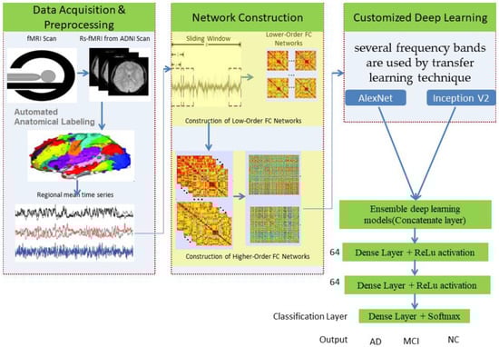
Figure 1.
Proposed model using deep networks.
The SPM12 software [27] and the toolboxes DPARSF (Data Processing Assistant for rsMRI) [28] and REST (Resting-state fMRI Data Analysis Toolkit) [29] were used to process the input scans. The initial ten volumes were removed to permit the dynamic equilibrium in each subject. Normalization for images has been performed, by which they were normalized from 0 to 1. We used the Inception V2 architecture [30] to identify abnormalities in the brain and detect them, leading to better results with less computational effort. The primary aim of this network was to select a particular layer at each level. This Inception V2 network uses a single filter size on the input brain MRI image (1 × 1) for which max pooling action is involved as a result of this inclusion.
This neuro-dynamic functional network provided better accuracy, sensitivity, and specificity, apart from being speedy and efficient for detecting AD using rs-fMRI images. The ADNI image dataset’s performance has been evaluated using various metrics, such as recall, specificity, and overall accuracy.
1. Disease Identification method: This is used to classify AD images collected by a medical expert during screening/monitoring programs.
2. Computer-Assisted Diagnosis: These methods are used to find the chances of disease based on rs-fMRI image changes.
3. Biomarkers: These are used for evaluating AD disease according to its severity.
This paper aimed to instigate an ML and CNN method for classifying AD from normal controls.
3.3. Methods
3.3.1. Customized AlexNet
The final three layers are replaced to solve the issue and achieve maximum accuracy. The last three layers of AlexNet—FC, SoftMax, and classification layer—replace the pre-trained network. These layers with the altered hyperparameters were eventually included by fine-tuning the previous layers and training the new layer of the AlexNet model using the ADNI dataset. The pre-trained model improved classification using the extensive ImageNet database using the feature extraction method. Minor tweaks are needed for the pre-trained parameters to adjust to the new MRI brain images. The modified hyperparameters define a small portion of the freshly transferred network.
Transfer learning is an essential statistical model for developing an efficient DL strategy. The critical regions of the brain can be recognized from MRI images by using newly updated parameters in a pre-trained network. These models have good convergence and are primarily used to extract the features and their classification. For this parameter learning, stochastic gradient descent with momentum optimizer is used.
As an extension to CNNs, the customized AlexNet architecture was developed to be competitive at the object detection task. Our proposed model achieves good performance using three bands without any external feature selection, reducing the task of exhaustive search using a set of heuristic approaches.
3.3.2. Customized Inception V2
In this section, the Inception V2 CNN architecture is presented. For AD detection, TI-weighted MR images and non-invasive methods are used.
The Inception V2 architecture being shown may identify abnormalities in the brain and detect them, leading to better results with less computational effort. The main goal of this network is to select a particular layer at each level. This Inception V2 network utilizes a single filter size on the input brain MRI image (a1 × a1). A max-pooling action is included as a result of the inclusion. The inception V2’s four pipes operate simultaneously. The architecture employs (1 × 1 × 1) filters in the first block to decrease the network by reducing the dimensions. The network begins with three convolutions dimension (a1 × a1 × a1, b3 × b3 × b3) matrix, which is comparable to the traditional network approaches (c5 × c5 × c5), (a1 × b3), and (c3 × 1). The filter size in the conventional network modal is (b3 × b3), which is divided into (a1 × b3) and (b3 × a1) convolutions. As an example, convolutions in the form of (b3 × b3) or (c5 × c5) are comparable to convolutions in the form of (a1 × b3) or (a1 × c5) and need less computation than (b3 × b3) dimension convolutions. In addition, the network comprises only two convolutions (a1 × a1 × a1); in the third part, it has only the pooling layer, and the fourth has only (a1 × a1 × a1) filters of convolution.
Similarly, all bands—aside from the max-pooling operation—begin with (a1 × a1 × a1) convolution filters. All conventional network layers are subjected to batch normalization to expedite training and reduce the risk of overfitting. After batch normalization is implemented, the convolution network improves and paves the way for data regularization in each network’s hidden layers; finally, a leaky ReLU function, the activation function, is implemented. The slope of this function is marginally negative at (0.01). The function’s slope is somewhat negative (0.01, or so on). The process is as follows in Equation (1):
where denoted as a negligible constant. The suggested Inception V2 has n properties, as shown in Figure 2, based on the input. In Figure 2, symbol indicates the multiplication operation. The primary advantage of the proposed model is the drastically reduced number of network parameters. The network’s primary goal is to transfer specific data from the origin to the target feature space. The primary notion of this network has changed the feature space of the spatial data from source to destination. The CONV 3D (s.m) represents the three-dimensional convolution with size (S) and filters (m), whereas the max pool three-dimensional (p.q) represents the three-dimensional max pool layer for down-sampling with the stride IQ and size of pool P. The convolution’s filter size has been divided into and convolutions. It is demonstrated that (a1 × b3) or (a1 × c5) convolutions, which perform (b3 × a1) or (c5 × a1) convolutions and are an output of the last layer, are comparable to (b3 × b3) or (c5 × c5) dimension convolutions. Finally, (b3 × b3), which is less expensive than other convolutions, is the concentration of two convolutions.
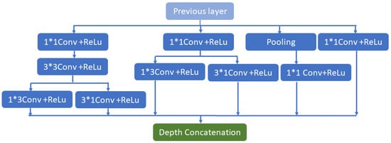
Figure 2.
Inception V2 network architecture.
The customized model still has its limitations. Pre-trained models such as VGG/inception often produce valuable features. The big difference is the formation of the problem, especially the VGG/inception, which was designed for multiclass classification, which means learning a lot of irrelevant information. All the issues can be solved by fine-tuning a pre-trained VGG argument with a few layers augmented with a few layers for binary classification, thus changing the intra-network AD vs. MCI, MCI vs. NL, and NL vs. AD. The weight stored internally can also be too much, requiring additional regularization. During the design of the network, we incorporated an Adam optimizer to require fewer parameters for tuning and implement a faster computation time.
In the traditional training method, the learning rate always remains the same. Recently, it has been suggested that the learning rate should be gradually changed, but this method has not been used in migration learning. Frequent changes in the learning rate not only accelerate the network convergence but also solve the problem that the loss value oscillates and is challenging to converge, with the learning weight also being gradually reduced. In top-level network training, better weight parameters are learned. A set of experiments are carried out to ensure the enhanced convergence rate of the model with improved recognition accuracy. The hyperparameter value is shown in Table 2.
Table 2.
Training Parameters for Customized AlexNet and Inception V2.
3.3.3. Ensemble Deep Learning Model (D2)
The customized models of Alexnet and Inception V2 described in the previous sections are separately tested on the dataset. The ensemble output is then created by adding the probabilities of each participant’s output.
The ensemble process merges various learning algorithms to gain their collective performance or to enhance the performance of current models by mixing different models to produce one trustworthy model. An ensemble framework works best when the participating systems are statistically varied because ensemble learning attempts to assemble complementing information from its numerous contributing models. Information fusion for improving classification performance is the primary justification for employing an ensemble learning model. To acquire a more reliable result, models trained using various data distributions related to the same set of classes are used while making predictions. The primary sources of error in learning models are noise, variation, and bias. Deep learning (DL) algorithms are accurate and stable due to the ensemble methods’ capacity to reduce these error-causing elements. SVM and KNN are two different learning methods. SVM makes the quite restricted assumption that a hyperplane separates the data points. In contrast, KNN attempts to approximate the underlying distribution of the data in a non-parametric way.
4. Experimentation Setup and Results Analysis
A typical Windows 10 system with 8 GB ram is used to develop an automated tool in MATLAB for the comparison of the results. The pre-processing steps of ADNI subjects are given in Section 2. The same input images are provided to all the transformations to get an unbiased estimation of their performance. One hundred fifty-three brain subjects are chosen and utilized for this purpose. Tenfold cross-validation is used for calculating the accuracies. The number of cross-validation sets is created from the entire dataset, and the result averaged precision from all those sets. The input array used for the deep learning models varies for different low frequencies. The slow4 features are resized to 50 × 50, slow5 features are resized to 60 × 60, and full-band features are resized to 110 × 110. This size is fixed based on the number of corresponding features. Figure 3 illustrates the entire execution process model.
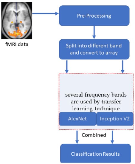
Figure 3.
The overall process of the execution model.
4.1. Performance Analysis
Performance analysis is necessary to evaluate the performance of any classification system. The tests are conducted in the following ways: three external bands, such as slow4, slow5, and full-band, are used to extract the dataset’s features.
Specificity: It correctly identifies negatively labelled classes using Equation (2).
Recall/Sensitivity: It identifies correctly positive labelled classes by using Equation (3)
Accuracy: It is an overall accuracy of true positive and negative out of the total number of observations that are examined by using Equation (4),
4.2. Result Analysis
To provide an unbiased evaluation, repeated tenfold cross-validation is observed, and the mean results are presented in this section. This study demonstrates the customized AlexNet, InceptionNet, and D2 stacked models. The images were normalized from 0 to 1. The Training Parameters for AlexNet and InceptionNet models are given in Table 2.
Table 3 lists the performance of customized AlexNet, InceptionNet, and D2 models using slow4, slow5, and full-band features. Their corresponding area under the curve (AUC) is plotted in Figure 4. With AlexNet, slow5 parts give the highest performance. For the AD again NL dataset, the majority baseline classification performance is 93.34%, and the AUC is 0.9488. For the MCI vs. NL dataset, the majority baseline classification accuracy is 76.56%, and for the AUC is 0.76.03. For the AD vs. MCI dataset, the majority baseline classification accuracy is 76.34%, and the AUC is 0.7780.
Table 3.
Summarizes the performance of customized AlexNet, InceptionNet, and D2 models using slow4, slow5, and full-band features.
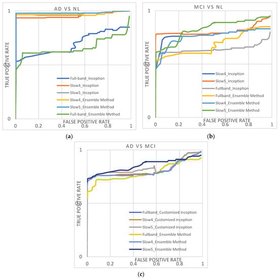
Figure 4.
(a–c) shows the ROC curve obtained from the AD/NL, MCI/NL, and AD/MCI.
InceptionNet trained with slow5 frequencies reaches the highest performance. For the AD vs. NL dataset, the baseline classification accuracy/AUC is 94.47%/0.9518, and for the MCI vs. NL dataset, the majority baseline classification accuracy/AUC is 79.67.47%/0.7989. For the AD vs. MCI dataset, the majority baseline classification accuracy/AUC is 80.45%/0.8145.
The D2 model with slow5 frequencies achieves the highest performance compared to all the other features. For the AD vs. NL dataset, the baseline classification accuracy/AUC is 96.61%/0.9663; for the MCI vs. NL dataset, the majority baseline classification accuracy/AUC is 81.87%/0.8221, and for the AD vs. MCI dataset, the majority baseline classification accuracy/AUC is 82.67%/0.8445. Among the three features, the slow4 and full-band perform lower than the slow5 frequencies for all the classification tasks. Additionally, it is noted that the D2 model outperforms better than other conventional models. It shows the diversity of the results produced using the AlexNet and InceptionNet models.
Next, the results are compared with conventional ML algorithms and are furnished in Table 4. The performance of our ensemble model outperforms the machine learning algorithms by 5–9%. It is also highlighted that other research also indicates that slow5 features perform better than using slow4 or full-band frequencies. The hyperparameter value is shown in Table 5.
Table 4.
Compares the performance of KNN and SVM model using slow4, slow5, and full-band features with traditional machine learning models.
Table 5.
Training parameters for SVM and KNN.
5. Discussion
In this study, dynamic neuro-functional deep ensemble networks are proposed and implemented to predict several AD periods, including the MCI (prodromal stage), using different frequency signals of rs-fMRI. In the three features (slow4, slow5, and full-band frequencies), slow5 achieves the top performance using the D2 model, with an accuracy/AUC of 96.61% for differentiating AD from NL subjects. In the D2 model trained for the MCI vs. NL task, the accuracy/AUC is 81.87%/0.8221, and for the AD vs. MCI task, the accuracy/AUC is 82.67%/0.8445 with the D2 model. The results in Figure 5 and Table 6 illustrate that the full-band and slow4 frequencies showed no substantial increase in accuracy. However, the slow5 features yield better performance when compared to the other two components. According to [20], slow5 features capture more discriminatory atrophies in different AD classifications. Our work is wholly automated. There is no need for feature selection.
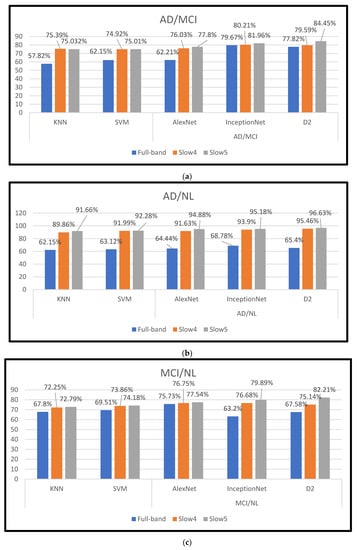
Figure 5.
(a–c) shows the different frequency bands obtained from the AD vs. MCI, AD vs. NL, and MCI vs. NL.
Table 6.
Compares the performance of fMRI-based recent methods with our proposed D2 model.
Furthermore, other works investigated fMRI neuroimaging modalities to identify regions with different levels of atrophy for the various AD classifications. It is noted that the additional training and testing of data used in other research make it difficult to compare our proposed method directly. The current methods use different features/feature selection in exploring various binary classifications in AD/MCI; the performance of multiple spans is illustrated in Table 6. The results from Table 6 indicate that dynamic neuro-functional deep learning ensemble networks with slow5 frequencies achieve better classification performance than other machine learning methods, including those performed in [31,32]. Gaussian/Regression models are used in most of the previous brain network models. Additionally, KNN and SVM classifiers use Fisher score feature selection to pick relevant features [15,33], and SVM with two kernels (radio basis functions and polynomial) are used along with the Fisher score features reaching 90% accuracy, whereas the linear kernel yield 100% performance. For the same Fisher characteristics, the KNN provides an accuracy of 87.5%. KNN and SVM classification algorithm models are used to analyze and classify AD diseases.
In machine learning, the supervised model k-Nearest Neighbors (KNN) is used. Supervised learning is the process through which a model learns from data that has been labelled. A set of input items and output values are fed into a supervised learning model. The method is then trained using the data to figure out how to translate the inputs into the required outputs, enabling it to forecast data that has not yet been observed. We must configure several basic settings for KNN.
5.1. SVM Parameter Setup
The parameter setup for SVM with a fixed number of neighbors is five. Gamma and c are SVM parameters for the Radial Basis Function (RBF) kernel. With low values signifying “far” and big values suggesting “near,” the γ parameter indicates the range of a particular training example’s influence. The model’s support vector samples’ radius of influence can be compared to the inverse of the γ parameters. The C parameter compromises good training sample classification for an increase in the margin of the decision function. Greater values of C can tolerate a smaller margin if the decision function is more accurate at correctly detecting all training points. A lower C reduces the training accuracy at the expense of a more significant margin and, hence, a more straightforward decision function. Our suggested dynamic neurofunctional deep ensemble networks demonstrate equal good performance in the prediction of numerous stages of AD when compared to other cutting-edge techniques.
The Brain-Connectivity networks, VGG19 [31], ResNet50 [33], Densenet121 [34], C3d [35], and C3d-LSTM [35], show good performance for the classifications. However, it is noted that the training set consists of both baseline and longitudinal images, and optimization parameters such as L1 and L2 regularization are needed to set up these networks. When compared with these models, it can be said that our work shows good compatible accuracy for all the classifications. This work reveals that there exist unique discriminatory frequency values in different bands, which is a major factor in determining the performance of our proposed research work. We have discussed the accuracies of different conventional ML and recent DL models on fMRI-based datasets in Table 6. In addition, our technique has an inherent feature selection, a deciding factor for improved accuracy. It is highlighted that our method requires less parameter optimization and is fully automated. This makes our method distinct from all the other methods.
From the last ten years, the different network approaches were used. In that, most authors use fewer datasets with low-frequency time series data and achieve more than 90% accuracy with varying band levels.
Our ensemble model also required fewer epochs during training; however, because of the large number of kernels at the first and second layers, the number of parameters is very high, increasing the model’s time complexity. Comparing this model to other feature extraction and classification models, the rs-fMRI slice technique effectively reduces the complexity of pre-processing. The drawbacks found in the low-order neurodynamics precisely manipulate the mono-band frequency span of rs-fMRI, leaving out the high-order neurodynamics. We propose an automated AD system to overcome these issues by developing a high-order neuro-dynamic functional network using various bands. The confusion matrix of AD is obtained as a 2 ∗ 2 matrix from the experiments performed with the segmentation and classification.
Table 7 presents the confusion matrix of our proposed model. From this, out of twenty subjects, the classifier predicted fourteen subjects as one correctly, and six subjects were misclassified as zero.
Table 7.
Confusion matrix of AD/NL classification.
Table 8 presents the confusion matrix of our proposed model. From this, out of twenty subjects, the classifier predicted fourteen subjects as one correctly, and six subjects were misclassified as zero.
Table 8.
Confusion matrix of MCI/NL classification with the hippocampal region.
Table 9 presents the confusion matrix of our proposed model. From this, out of twenty subjects, the classifier predicted fifteen subjects as one correctly, and five subjects were misclassified as zero. The classifier’s efficiency is evaluated from the 2 ∗ 2 matrix for each region through TP, FP, TN, and FN. The results obtained give desired performances with the testing subjects. The observations show no significant differences over “AD vs. NL, MCI vs. NL and AD vs. MCI”. Hence it portrays that the proposed model outperforms the multiclass classification problems.
Table 9.
Confusion matrix of AD/MCI classification with the hippocampal region.
5.2. Limitations of the Work
The classification of medical images is a fundamental and significant issue in computer innovation, which has undergone much research over the past few decades. Even though the reliability of various medical image classification methods has significantly increased, these methods may not offer correct AD because of their non-universality, vulnerability to illumination and spoofing effects, and insufficient accuracy via the poor data quality. Therefore, in many real-world applications, standard medical picture categorization may not be able to deliver the needed performance. In this study, we solely used the ADNI dataset to categorize the three frequency ranges of the various phases of AD. The dataset we used here is small for the entire experimentation. Additionally, this work solely uses traditional methods for AD classification, such as SVM and KNN, instead of alternative techniques.
6. Conclusions
In this work, the dynamic neuro-functional deep ensemble networks use various frequencies in resting-state fMRI to diagnose different stages of AD from real-time ADNI datasets. The excellent performance is achieved with our proposed D2 model using three bands (slow4, slow5, and full-band) without any external feature selection, and it is a combination of two deep learning models. Among the three bands evaluated, the results show that the slow5 features, when trained with various customized Alex and Inception networks, perform better for AD/MCI classifications. It is also mentioned that additional studies are required to develop these networks to increase the precision of AD classifications. We have contrasted our networks against established machine learning techniques and more contemporary deep learning techniques. It demonstrates that rs-fMRI multi-band characteristics have a higher potential for being AD biomarkers than single-band features. It is also noted that more research is needed to optimize these networks to improve the accuracy of AD classifications. We have compared our networks with traditional machine learning methods and current deep learning methods. Our study shows that the multi-band features of rs-fMRI have more potential to be AD biomarkers than single-band features. Additionally, the performance of the proposed ensemble model outperforms the conventional ML algorithms by 5–9%. The proposed model is less complex to train and requires fewer hardware resources. Furthermore, the proposed model had surpassed in terms of accuracy the various existing models. In the future, we aim to test and apply this model on a more extensive and richer dataset. Moreover, we hope to implement single-cell transcriptome data using variational neighborhood preserving quantum embeddings and deep learning. In the future, the use of image augmentation for AD classification may be added with different image augmentation methods such as flipping, padding, etc.
Author Contributions
Conceptualization, S.K.S.; methodology, S.K.S. and N.M.; validation, M.R. and R.R.; formal analysis, N.M., S.B. and N.A.; writing—original draft preparation, S.K.S.; writing—review and editing, R.R., M.R. and S.B., supervision, N.M. Funding Acquisition, S.B. All authors have read and agreed to the published version of the manuscript.
Funding
This research is supported by Princess Nourah bint Abdulrahman University Researchers Supporting Project number (PNURSP2023R195) Princess Nourah bint Abdulrahman University, Riyadh, Saudi Arabia.
Data Availability Statement
Data in this research paper will be shared upon request with the corresponding author. Data used in the preparation of this article were obtained from the Alzheimer’s Disease Neuroimaging Initiative (ADNI)database (https://ida.loni.usc.edu/home/projectPage.jsp?project=ADNI, accessed on 1 September 2022). As such, the investigators within the ADNI contributed to the design and implementation of ADNI and/or provided data but did not participate in analysis or writing of this report. A complete listing of ADNI investigators is available at: https://adni.loni.usc.edu/wp-content/uploads/how_to_apply/ADNI_Acknowledgement_List.pdf (accessed on 1 September 2022).
Acknowledgments
This research is supported by Princess Nourah bint Abdulrahman University Researchers Supporting Project number (PNURSP2023R195) Princess Nourah bint Abdulrahman University, Riyadh, Saudi Arabia.
Conflicts of Interest
The authors declare no conflict of interest.
References
- Burns, A.; Iliffe, S. Alzheimer’s disease. BMJ 2009, 338, b158. [Google Scholar] [CrossRef] [PubMed]
- McKhann, G.; Drachman, D.; Folstein, M.; Katzman, R.; Price, D.; Stadlan, E.M. Clinical diagnosis of Alzheimer’s disease: Report of the NINCDS-ADRDA Work Group under the auspices of Department of Health and Human Services Task Force on Alzheimer’s Disease. Neurology 1984, 34, 939–944. [Google Scholar] [CrossRef] [PubMed]
- Querfurth, H.W.; Laferla, F.M. Alzheimer’s Disease. J. Med. 2011, 362, 329–344. [Google Scholar] [CrossRef]
- Li, X.; Li, Y.; Li, X. Predicting Clinical Outcomes of Alzheimer’s Disease from Complex Brain Networks. Int. Conf. Adv. Data Min. Appl. 2017, 3, 519–525. [Google Scholar]
- National Institute for Health and Care Excellence. Dementia: Assessment, management and support for people living with dementia and their carers. Grants Regist. 2018, 1–43. Available online: www.nice.org.uk/guidance/ng97 (accessed on 1 September 2022).
- Li, T.; Li, J.; Liu, J.; Huang, M.; Chen, Y.-W.; Bhatti, U.A. Robust watermarking algorithm for medical images based on log-polar transform. EURASIP J. Wirel. Commun. Netw. 2022, 2022, 1–11. [Google Scholar] [CrossRef]
- Mao, S.; Zhang, C.; Gao, N.; Wang, Y.; Yang, Y.; Guo, X.; Ma, T. A study of feature extraction for Alzheimer’s disease based on resting-state fMRI. In Proceedings of the 2017 39th Annual International Conference of the IEEE Engineering in Medicine and Biology Society (EMBC), Jeju, Republic of Korea, 11–15 July 2017; pp. 517–520. [Google Scholar] [CrossRef]
- Tripoliti, E.E.; Fotiadis, D.I.; Argyropoulou, M. A supervised method to assist the diagnosis and monitor progression of Alzheimer’s disease using data from an fMRI experiment. Artif. Intell. Med. 2011, 53, 35–45. [Google Scholar] [CrossRef] [PubMed]
- Dachena, C.; Casu, S.; Lodi, M.B.; Fanti, A.; Mazzarella, G. Application of MRI, fMRI and Cognitive Data for Alzheimer’s Disease detection. In Proceedings of the 2020 14th European Conference on Antennas and Propagation (EuCAP), Copenhagen, Denmark, 15–20 March 2020. [Google Scholar] [CrossRef]
- Wang, Z.; Zheng, Y.; Zhu, D.C.; Bozoki, A.C.; Li, T. Classification of Alzheimer’s Disease, Mild Cognitive Impairment and Normal Control Subjects Using Resting-State fMRI Based Network Connectivity Analysis. IEEE J. Transl. Eng. Health Med. 2018, 6, 1–9. [Google Scholar] [CrossRef]
- Hojjati, S.H.; Ebrahimzadeh, A.; Babajani-Feremi, A. Identification of the Early Stage of Alzheimer’s Disease Using Structural MRI and Resting-State fMRI. Front. Neurol. 2019, 10, 904. [Google Scholar] [CrossRef]
- Zhang, Z.; Ding, J.; Xu, J.; Tang, J.; Guo, F. Multi-Scale Time-Series Kernel-Based Learning Method for Brain Disease Diagnosis. IEEE J. Biomed. Health Inform. 2020, 25, 209–217. [Google Scholar] [CrossRef] [PubMed]
- Bi, X.-A.; Jiang, Q.; Sun, Q.; Shu, Q.; Liu, Y. Analysis of Alzheimer’s Disease Based on the Random Neural Network Cluster in fMRI. Front. Neuroinformatics 2018, 12, 60. [Google Scholar] [CrossRef] [PubMed]
- Odusami, M.; Maskeliūnas, R.; Damaševičius, R.; Krilavičius, T. Analysis of Features of Alzheimer’s Disease: Detection of Early Stage from Functional Brain Changes in Magnetic Resonance Images Using a Finetuned ResNet18 Network. Diagnostics 2021, 11, 1071. [Google Scholar] [CrossRef]
- Cheng, J.; Liu, Z.; Guan, H.; Wu, Z.; Zhu, H.; Jiang, J.; Wen, W.; Tao, D.; Liu, T. Brain Age Estimation From MRI Using Cascade Networks With Ranking Loss. IEEE Trans. Med. Imaging 2021, 40, 3400–3412. [Google Scholar] [CrossRef]
- Amini, M.; Pedram, M.; Moradi, A.; Ouchani, M. Diagnosis of Alzheimer’s Disease Severity with fMRI Images Using Robust Multitask Feature Extraction Method and Convolutional Neural Network (CNN). Comput. Math. Methods Med. 2021, 2021, 1–15. [Google Scholar] [CrossRef]
- Ju, R.; Hu, C.; Zhou, P.; Li, Q. Early Diagnosis of Alzheimer’s Disease Based on Resting-State Brain Networks and Deep Learning. IEEE/ACM Trans. Comput. Biol. Bioinform. 2017, 16, 244–257. [Google Scholar] [CrossRef] [PubMed]
- Gupta, U.; Lam, P.K.; Steeg, G.V.; Thompson, P.M. Improved Brain Age Estimation With Slice-Based Set Networks. In Proceedings of the 2021 IEEE 18th International Symposium on Biomedical Imaging (ISBI), Nice, France, 13–16 April 2021; pp. 840–844. [Google Scholar] [CrossRef]
- Abrol, A.; Fu, Z.; Du, Y.; Calhoun, V.D. Multimodal Data Fusion of Deep Learning and Dynamic Functional Connectivity Features to Predict Alzheimer’s Disease Progression. In Proceedings of the 2019 41st Annual International Conference of the IEEE Engineering in Medicine and Biology Society (EMBC), Berlin, Germany, 23–27 July 2019; Volume 2019, pp. 4409–4413. [Google Scholar] [CrossRef]
- Wang, M.; Lian, C.; Yao, D.; Zhang, D.; Liu, M.; Shen, D. Spatial-Temporal Dependency Modeling and Network Hub Detection for Functional MRI Analysis via Convolutional-Recurrent Network. IEEE Trans. Biomed. Eng. 2019, 67, 2241–2252. [Google Scholar] [CrossRef] [PubMed]
- Shi, Y.; Zeng, W.; Deng, J.; Nie, W.; Zhang, Y. The Identification of Alzheimer’s Disease Using Functional Connectivity Between Activity Voxels in Resting-State fMRI Data. Adv. Intell. Technol. Dement. 2020, 8, 1400211. [Google Scholar] [CrossRef]
- Khatri, U.; Kwon, G.-R. Classification of Alzheimer’s Disease and Mild-Cognitive Impairment Base on High-Order Dynamic Functional Connectivity at Different Frequency Band. Mathematics 2022, 10, 805. [Google Scholar] [CrossRef]
- Helaly, H.A.; Badawy, M.; Haikal, A.Y. Deep Learning Approach for Early Detection of Alzheimer’s Disease. Cogn. Comput. 2021, 14, 1711–1727. [Google Scholar] [CrossRef]
- Turkson, R.E.; Qu, H.; Mawuli, C.B.; Eghan, M.J. Classification of Alzheimer’s Disease Using Deep Convolutional Spiking Neural Network. Neural Process. Lett. 2021, 53, 2649–2663. [Google Scholar] [CrossRef]
- Zhang, Y.; Zhang, H.; Chen, X.; Lee, S.-W.; Shen, D. Hybrid High-order Functional Connectivity Networks Using Resting-state Functional MRI for Mild Cognitive Impairment Diagnosis. Sci. Rep. 2017, 7, 6530. [Google Scholar] [CrossRef] [PubMed]
- Arafa, D.A.; Moustafa, H.E.-D.; Ali-Eldin, A.M.T.; Ali, H.A. Early detection of Alzheimer’s disease based on the state-of-the-art deep learning approach: A comprehensive survey. Multimed. Tools Appl. 2022, 81, 23735–23776. [Google Scholar] [CrossRef]
- Neuroimaging B Members & Collaborations of the WCFH. SPM, Statistical Parametric Mapping n.d. Available online: http://www.fil.ion.ucl.ac.uk/spm (accessed on 1 September 2022).
- Yan, C.; Zang, Y. DPARSF: A MATLAB toolbox for “pipeline” data analysis of resting-state fMRI. Front. Syst. Neurosci. 2010, 4, 13. [Google Scholar] [CrossRef] [PubMed]
- Song, X.-W.; Dong, Z.-Y.; Long, X.-Y.; Li, S.-F.; Zuo, X.-N.; Zhu, C.-Z.; He, Y.; Yan, C.-G.; Zang, Y.-F. REST: A Toolkit for Resting-State Functional Magnetic Resonance Imaging Data Processing. PLoS ONE 2011, 6, e25031. [Google Scholar] [CrossRef] [PubMed]
- Bose, S.R.; Kumar, V.S. Efficient inception V2 based deep convolutional neural network for real-time hand action recognition. IET Image Process. 2020, 14, 688–696. [Google Scholar] [CrossRef]
- Challis, E.; Hurley, P.; Serra, L.; Bozzali, M.; Oliver, S.; Cercignani, M. Gaussian process classification of Alzheimer’s disease and mild cognitive impairment from resting-state fMRI. Neuroimage 2015, 112, 232–243. [Google Scholar] [CrossRef]
- De Vos, F.; Koini, M.; Schouten, T.M.; Seiler, S.; van der Grond, J.; Lechner, A.; Schmidt, R.; de Rooij, M.; Rombouts, S.A.R.B. A comprehensive analysis of resting state fMRI measures to classify individ-ual patients with Alzheimer’s disease. Neuroimage 2018, 167, 62–72. [Google Scholar] [CrossRef]
- Vaithinathan, K.; Parthiban, L. A Novel Texture Extraction Technique with T1 Weighted MRI for the Classification of Alzheimer’s Disease. J. Neurosci. Methods 2019, 318, 84–99. [Google Scholar] [CrossRef]
- Ramzan, F.; Khan, M.U.G.; Rehmat, A.; Iqbal, S.; Saba, T.; Rehman, A.; Mehmood, Z. A Deep Learning Approach for Automated Diagnosis and Multi-Class Classification of Alzheimer’s Disease Stages Using Resting-State fMRI and Residual Neural Networks. J. Med. Syst. 2019, 44, 37. [Google Scholar] [CrossRef]
- Duc, N.T.; Ryu, S.; Qureshi, M.N.I.; Choi, M.; Lee, K.H.; Lee, B. 3D-Deep Learning Based Automatic Diagnosis of Alzheimer’s Disease with Joint MMSE Prediction Using Resting-State fMRI. Neuroinformatics 2019, 18, 71–86. [Google Scholar] [CrossRef]
- Parmar, H.S.; Nutter, B.; Long, R.; Antani, S.; Mitra, S. Deep learning of volumetric 3D CNN for fMRI in Alzheimer’s disease classification. In Proceedings of the Medical Imaging 2020: Biomedical Applications in Molecular, Structural, and Functional Imaging, Houston, TX, USA, 15–20 February 2020; Volume 11317, p. 113170C. [Google Scholar] [CrossRef]
- Al-Khuzaie, F.E.K.; Bayat, O.; Duru, A.D. Diagnosis of Alzheimer Disease Using 2D MRI Slices by Convolutional Neural Network. Appl. Bionics Biomech. 2021, 2021, 1–9. [Google Scholar] [CrossRef] [PubMed]
- Bhaskaran, B.; Anandan, K. Assessment of Graph Metrics and Lateralization of Brain Connectivity in Progression of Alzheimer’s Disease Using fMRI. Int. J. Softw. Sci. Comput. Intell. 2017, 9, 46–66. [Google Scholar] [CrossRef]
- Luo, Y.; Sun, T.; Ma, C.; Zhang, X.; Ji, Y.; Fu, X.; Ni, H. Alterations of Brain Networks in Alzheimer’s Disease and Mild Cognitive Impairment: A Resting State fMRI Study Based on a Population-specific Brain Template. Neuroscience 2020, 452, 192–207. [Google Scholar] [CrossRef]
- Dennis, E.L.; Thompson, P.M. Functional Brain Connectivity Using fMRI in Aging and Alzheimer’s Disease. Neuropsychol. Rev. 2014, 24, 49–62. [Google Scholar] [CrossRef] [PubMed]
- He, K.; Zhang, X.; Ren, S.; Sun, J. Deep residual learning for image recognition. In Proceedings of the IEEE Computer Society Conference on Computer Vision and Pattern Recognition (CVPR), Las Vegas, NV, USA, 27–30 June 2016; pp. 770–778. [Google Scholar] [CrossRef]
- Huang, G.; Liu, Z.; Van Der Maaten, L.; Weinberger, K.Q. Densely connected convolutional networks. In Proceedings of the 30th IEEE Conference on Computer Vision and Pattern Recognition, CVPR 2017, Honolulu, HI, USA, 21–26 July 2017; pp. 2261–2269. [Google Scholar]
- Li, W.; Lin, X.; Chen, X. Detecting Alzheimer’s disease Based on 4D fMRI: An exploration under deep learning framework. Neurocomputing 2020, 388, 280–287. [Google Scholar] [CrossRef]


Disclaimer/Publisher’s Note: The statements, opinions and data contained in all publications are solely those of the individual author(s) and contributor(s) and not of MDPI and/or the editor(s). MDPI and/or the editor(s) disclaim responsibility for any injury to people or property resulting from any ideas, methods, instructions or products referred to in the content. |
© 2023 by the authors. Licensee MDPI, Basel, Switzerland. This article is an open access article distributed under the terms and conditions of the Creative Commons Attribution (CC BY) license (https://creativecommons.org/licenses/by/4.0/).