Ground Risk Estimation of Unmanned Aerial Vehicles Based on Probability Approximation for Impact Positions with Multi-Uncertainties

Abstract

In this paper, a methodology to assess ground risk with multi-uncertainties is introduced, which is associated with a major unmanned aerial vehicle (UAV) in-flight incident. In the assessment model, random factors are taken into account including uncertainty in the drag force, uncertainty in the UAV velocity, and the random effects of local wind. The probability distribution of impact positions is first estimated by using a second-order drag model with probabilistic assumptions regarding the least well-known parameters. Then, an approach for modeling and estimating the ground risks is presented, in which the ground casualties are set as the safety index. In the multifactor risk estimation model, ground casualty areas covered by the UAVs’ debris are determined. Correspondingly, the probability of fatal injuries to people is derived by addressing the protection effects, impact energy, and energy threshold a person can sustain. Further, four kinds of sheltering effects are defined. Finally, the affected area on the ground is partitioned into six zones, taking into consideration the density and distribution of the local population. Case studies are conducted for fixed-wing and rotary-wing UAVs. Risk levels on the ground are obtained and compared with the widely accepted target safety level of manned aircrafts.

1. Introduction

Unmanned aerial vehicles (UAVs) are a new, rapidly growing technology in the aviation industry, which have been widely used in civil and military fields [1,2,3]. However, there are still a number of challenges which inevitably result in the imposition of many operation restrictions [4,5,6]. Out of all these challenges, the most significant is the absence of a suitable regulatory framework which can be used for governing the safety of UAV operations. Recently, a risk-based approach has been adopted for the development of a regulatory framework for UAVs, which are recognized by the Federal Aviation Administration (FAA) and the European Aviation Safety Authority (EASA) [7,8]. There are two kinds of risks related to UAV operations. One is the midair collision between a UAV and another manned or unmanned aircraft, and the other is the collision with people or structures situated on the ground that is caused by the failure of the UAV. The scope of this paper is limited to the latter of these two hazards and focuses on the risks imposed by a UAV’s crash to the ground.

Currently, many models and algorithms for ground safety assessments have been proposed, which are mainly built upon the well-studied subject of third-party risk associated with UAV operations. The risk to people on the ground that is caused by a UAV’s failure is the most important. Lazatin [9] and Lum [10] estimated the fatalities due to ground and mid-air collisions by incorporating the population density, population distribution, and sheltering factors, and their results were reliably used in confirming the insurance liability for various UAV operation cases. In a similar way, a conceptual third-party risk model was proposed by Aalmoes [11] to estimate the potential impact area and the consequence area on the ground. Clothier et al. [12] introduced quite a different approach, in which various type categories of UAVs based on their own kinetic energy and impact severity (injury or fatalities) were assigned. By considering the initial failure location of a UAV as well as satellite imagery and census information, Lum [13] and Ford [14] simulated the impact areas on the ground to estimate the number of collisions with a bystander per flight hour. Furthermore, by calculating the kinetic energy of a crashed UAV at the impact point on the ground, Weibel [15] and Burke [16] estimated the casualties on the ground considering the UAV’s ground impact frequency and ground population density, leading to results that are more reliable and useful. By comparing past research, Melynk et al. [17] used the index fatality rates from general aviation crashes, which were obtained from historical data, to evaluate the casualties on the ground. The model was also validated by using historical data to quantize the casualty prediction.

Most of the existing research only deals with the risk that results from the UAV’s crash to the ground and neglects the complete descending process in which many indispensable influences are dismissed. Additionally, the current research hardly analyzes the randomness during the whole process that is caused by the failure event happening in the air. All the uncertainties that may appear during the descent are not taken into account in the risk estimation model, which accordingly makes the assessment unreliable and the results meaningless, so they cannot be further used in actual applications, especially for the development of a regulatory framework.

In this paper, a ground safety assessment algorithm is proposed for when a UAV failure event happens in the air. The associated probability distributions of impact positions on the ground are estimated using a second-order drag model. In order to describe the descending process precisely, probabilistic assumptions regarding the least well-known parameters of the UAV flight are made. Random factors with multi-uncertainties are assigned in the risk estimation model, which includes uncertainty in the drag force, uncertainty in the velocity when a failure event happens, and uncertainty in the effects of local wind. Then, an effective approach for modeling and estimating the ground risks is presented, in which the ground casualties caused by the UAV’s crash are selected as the safety index to evaluate the level of hazards and threats. In the designed multifactor risk model, ground casualty areas covered by the UAV’s debris are determined using the parameters of the descending process and characteristics of human beings. Probability of fatal injuries is another factor which is derived by addressing the protection effects provided by the ground, the impact energy of the UAV, and the corresponding energy threshold a person can hold. Four kinds of sheltering effects are defined to quantize the protections of different ground features. In order to make the quantization more precise, the ground areas are partitioned into six different zones. The statistical data are imported to describe the density and reliable distribution of the local population. Official territory and population data of the operation airspace are incorporated, as well as UAV self-properties. The risk levels in different zones on the ground are calculated and compared with the widely accepted target safety level of manned aircrafts.

The remainder of this paper is organized as follows: A description of the ground risk estimation problem is given in Section 2. Section 3 describes the detailed modeling and realization of the ground safety assessment that is used in this work. Simulations and verification with actual operation scenarios and official data are presented in Section 4. Finally, the paper is concluded in Section 5.

2. Problem Description

It is becoming more and more crucial to assess and estimate the ground risk imposed by a UAV’s failure, especially for airspace integration in the future. In order to perform the safety assessment and risk estimation accurately, two kinds of problems are indispensable that need to be addressed in detail. The first one is the calculation of impact positions on the ground when a UAV fails in the air, and the other one is the modeling of ground features where a UAV may crash. This is a complicated process that involves many factors that should not be neglected. In this paper, we mainly focus on the two problems to better carry out the safety assessment and estimation of the associated ground risk caused by a UAV falling from a fixed flying altitude. It should be noted that all UAVs should only operate at the legal altitude that is specified by the local government. The detailed problem description of this work can be found in Figure 1.

When a UAV failure event happens in the air, the UAV will fall to the ground, leading to many possible impact positions. Impact positions determine the area on the ground that could be covered by a UAV’s crash, which is called the casualty area. The calculation of exact impact positions becomes an important problem for accurately estimating risk. As shown in Figure 1, ground impact positions are highly affected by many factors. Especially during the descent after a UAV’s failure, the primary forces acting on the UAV body in a ballistic descent are gravity and drag force. In this way, the dimensions and dynamics of a UAV play an important role. For example, the current total UAV mass and its wingspan could both greatly influence the descent. As another example, the UAV’s dynamics, including initial horizontal and vertical speeds when the failure event happens, could change the descending path and make the impact positions quite uncertain.

In the estimation of impact positions, many uncertainties exist. The first concerns the UAV’s movement. At the time of the event, it is difficult to obtain the exact velocity of the corresponding UAV. Due to current UAV applications, most flights are preplanned with an expected velocity at any given point on the flying path. However, due to the uncertainties in airspeed measurements and effects of the onboard controller attempting to maintain not just velocity, but also altitude and heading, the real velocity may vary from the expected value largely. These variations are quite difficult to predict and are therefore handled as a stochastic process. Additionally, there are uncertainties in the descent process. The drag force could cause the descent to occur in many different ways, as it is mainly determined by drag coefficient, drag area, and air density. In turn, the descent also depends on the drag coefficient and the frontal area facing the travel direction, which are inherently difficult to determine. In order to capture these descent uncertainties, it is reasonable to assume that the drag coefficient is a stochastic parameter and the frontal area is derived from some fraction of the UAV frontal area, as seen from the direction with the largest area.

The modeling of ground features makes sense for the risk estimation of ground impact. As given in Figure 1, ground area properties should be considered first, including various region sizes, the number of people located in the possible impact areas, and the kinds of buildings that may offer protection for human beings. Additionally, population distributions are fundamental to determine the ground risk levels. This is because the frequency of ground fatalities per UAV flight hour is the focus, and an index to evaluate the levels of safety in some specified zones is necessary. More people on the ground will increase the risk caused by a UAV’s crash and vice versa. Another factor that is necessary for the ground feature model is the effect of the surrounding environment. Different environments could protect people from being harmed or reduce the damage caused by a UAV’s hit. For example, reinforced concrete buildings, trees, or bare surfaces all contribute to risk levels in different ways.

Based on the physical knowledge of how a UAV falls, wind would increase the uncertainties in the risk estimation model because it can cause the UAV to deviate from the expected path. The quantitative definition of the effects that are generated by wind speed and wind direction becomes a key problem. Additionally, since the air velocity will not stay parallel to the UAV’s flight direction, the wind will change the ground impact locations from one dimension to two dimensions, covering a geographical area rather than just a line segment. Furthermore, the wind speed and direction are both variable all the time. Therefore, taking the wind effects as a stochastic process is feasible to quantify its uncertainty and randomness.

3. Modeling for Ground Safety Assessment

Based on the problem definitions in Section 2, a ground safety assessment model is introduced to give solutions for the estimation of ground impact positions and the derivation of ground features. Then, the modeling of the assessment and how to obtain the values of ground risks are described in detail at the end of this section.

3.1. Estimation of Horizontally Travelled Distance

The core step of estimating the possible ground impact positions is to find the horizontally travelled distance from the UAV’s failure point to the ground impact point. Many factors should be considered, as discussed in the Problem Description section. In this section, a second-order drag model is incorporated [18].

3.1.1. Kinematic Pattern of UAV’s Descent

It is known that when a UAV fails in the air, there are two primary forces acting on it, namely, gravity and drag force. The former is a constant and is a fixed value once the current mass is known. For the latter, there is a standard second-order model with velocities and shapes that is realistic to use for a crippled, descending aircraft [19]. In this model, drag force is proportional to the square of the moving velocity, making it obvious that it is the same for motion in all directions, even though the motion could be decomposed into horizontal and vertical directions. Without a loss of generality, to simplify the calculations, a compromising semi-decoupling assumption is made that allows for a closed-form solution, as well as a solution that is similar to the solution to the fully coupled 2D dynamic equations [18]. The standard second-order model for a UAV’s descent with drag forces is given in Equation (1).

$$m\dot{v}=mg-c\left|v\right|v$$

(1)

In the equation above, m is the current mass of the UAV and c is a variable that captures the drag coefficient, drag area, and air density. Typically, c can be calculated using Equation (2). In Equation (2), ρ is the air density, which is a constant, A is the frontal area of the UAV, and C_D stands for the drag coefficient. In the given model, C_D is defined as a stochastic parameter to completely solve for the descent uncertainties, as declared in Section 2.

$$c=0.5\cdot \rho \cdot A\cdot C_D$$

(2)

The velocity of a UAV can be generally divided into horizontal speed v_x, in which only positive values exist, and vertical speed v_y, in which downward is defined as positive. It is assumed that v_x > 0 and will monotonically decrease as there is no thrust force in the horizontal plane to push the UAV. In the same way, v_y asymptotically approaches a steady state value when gravity and drag force cancel each other out. With this assumption, Equation (1) can be approximated using Equation (3) correspondingly.

$$\left\{\begin{array}{l}m{\dot{v}}_x=-c\max (v_x,v_y)v_x\\ m{\dot{v}}_y=mg-c\left|v_y\right|v_y\end{array}\right.$$

(3)

Once the UAV’s initial horizontal speed v_x,i and initial vertical speed v_y,i are both given in advance, the horizontal speed v_x can then be obtained using Equations (4) and (5), which are both functions of time t.

$$v_x(t)=\frac{m{v}_{x,i}}{m+v_{x,i}ct}\hspace{1em}\hspace{1em}\hspace{1em}\hspace{1em}\hspace{1em}\hspace{1em}\hspace{1em}when\hspace{1em}{v}_x>v_y$$

(4)

$$v_x(t)=v_{x,i}\exp (-\frac{c}{m}{\displaystyle {\mathsf{\int }}_0^t{v}_y(\tau )d\tau })\hspace{1em}when\hspace{1em}{v}_x\le v_y$$

(5)

Similarly, the vertical speed v_y can also be expressed as a function of time t using Equations (6) and (7).

$$v_y(t)=\mathrm{\Gamma }\tan (g\gamma t+H_u)\hspace{1em}\hspace{1em}\hspace{1em}\hspace{1em}\hspace{1em}{v}_y(t)<0$$

(6)

$$v_y(t)=\mathrm{\Gamma }\tanh (g\gamma t+H_d)\hspace{1em}\hspace{1em}\hspace{1em}\hspace{1em}\hspace{1em}{v}_y(t)\ge 0$$

(7)

$$v_y(t)=\mathrm{\Gamma }\hspace{1em}\hspace{1em}\hspace{1em}\hspace{1em}\hspace{1em}\hspace{1em}\hspace{1em}\hspace{1em}\hspace{1em}\hspace{1em}\hspace{1em}\hspace{1em}{v}_y(0)=\mathrm{\Gamma }$$

(8)

In the equations above, H_d and H_u can be calculated using Equations (9) and (10), respectively.

$$H_d=\mathrm{arctanh}(v_{y,i}\gamma )$$

(9)

$$H_u=\arctan (v_{y,i}\gamma )$$

(10)

When the gravitational force and drag force are equal but with opposite signs, there would be a terminal velocity for the UAV, which is denoted as Γ. It can be calculated easily based on the physical theory given in Equation (11). γ is the reciprocal of Γ, namely, γ = 1/Γ.

$$\mathrm{\Gamma }=\sqrt{mg/c}=1/\gamma$$

(11)

3.1.2. Three Stages from UAV Failure to Ground Impact

In the proposed model, three stages are defined from the UAV failure event to ground impact. Stage one begins when a UAV failure happens and lasts until the moment when the UAV arrives at the highest altitude, namely, t_top. As analyzed above, if v_y,I > 0, then t_top = 0. Stage two occurs from the point of highest altitude to the moment when v_x = v_y, namely, the time t_c. The last stage is between t_c and the impact time t_im. For the model used in this paper, an upward motion for the failed UAV would happen if v_y,i < 0.

With a ballistic trajectory, the UAV may start with an upward motion, given v_y(t) < 0, but there is no doubt that it will always end with a downward motion. In this way, based on Equation (6), t_top can then be obtained using Equation (12).

$$t_{top}=-\frac{\mathrm{\Gamma }}{g}{H}_u$$

(12)

In order to include the situation that v_y,i > 0, Equation (12) with Equation (10) can be combined into Equation (13), where t_top can be further calculated.

$$t_{top}=-\frac{\mathrm{\Gamma }}{g}\arctan [\gamma \min (0,v_{y,i})]$$

(13)

In the model, all the vertically travelled distances during the three stages can be divided into two main categories, upward distance y_u(t) and downward distance y_d(t), both of which are variables with time t as denoted in Equations (14) and (15).

$$y_u(t)=-\frac{m}{c}\left\{\ln \left[\cos (g\gamma t+H_u)\right]-G_u\right\}$$

(14)

$$y_d(t)=\frac{m}{c}\left\{\ln \left[\cosh (g\gamma t+H_d)\right]-G_d\right\}$$

(15)

In the two equations above, G_u and G_d can be derived with Equations (16) and (17), respectively.

$$G_u=\ln \cos H_u=-\frac{1}{2}\ln \left[1+{(v_{y,i}\gamma )}^2\right]$$

(16)

$$G_d=\ln \cosh H_d=-\frac{1}{2}\ln \left[1-{(v_{y,i}\gamma )}^2\right]$$

(17)

In this way, the total time that lasts from stage two to stage three when a UAV’s failure event happens at a given flight altitude y can be expressed as t_drop and obtained with Equation (18).

$$t_{drop}(y)=\{\arccos \mathrm{h}[\exp (\frac{cy}{m}+G_d)]-H_d\}\frac{\mathrm{\Gamma }}{g}$$

(18)

Then, by combining Equation (13) with Equation (18), the total time t_im from a UAV’s failure to the ground impact can be determined with Equation (19).

$$t_{im}(y)=\left\{\begin{array}{l}{t}_{top}+t_{drop}\left[y+y_u(t_{top})\right]{|}_{H=G=0}\hspace{1em}\hspace{1em}\hspace{1em}{v}_{y,i}<0\\ t_{drop}(y)\hspace{1em}\hspace{1em}\hspace{1em}\hspace{1em}\hspace{1em}\hspace{1em}\hspace{1em}\hspace{1em}\hspace{1em}\hspace{1em}\hspace{1em}\hspace{1em}\hspace{1em}{v}_{y,i}\ge 0\end{array}\right.$$

(19)

Another parameter is the time when the horizontal speed v_x(t) is equal to the vertical speed v_y(t), which is denoted as t_c. Because of the assumption that v_x > 0 all the time, v_y(t) should also be positive at the time t_c. This helps to determine that Equations (4) and (7) can be utilized to calculate t_c. Since the equation tanh(at) = 1/t seems to have no closed-form solution, a truncation of the continued fraction for the hyperbolic tangent is used to approximate the time t_c, allowing Equation (5) to be used instead of Equation (4). In this situation, the following equation can be obtained:

$$v_y(t-t_{top})\approx \mathrm{\Gamma }\frac{g\gamma (t-t_{top})+H_d}{1+{[g\gamma (t-t_{top})+H_d]}^2}=\frac{m{v}_{x,i}}{m+v_{x,i}ct}=v_x(t)$$

(20)

As shown in Equation (20), if v_y,i < 0, H_d would be set as 0 and for v_y,i ≥ 0, we set t_top = 0. By solving Equation (20), the value of t_c will be obtained. After that, Equation (5) can be rewritten as follows:

$$v_x(t)=v_{x,i}\exp \left[-\frac{c}{m}{y}_d(t)\right]=v_{x,i}{e}^{G_d}\sec \mathrm{h}(g\gamma t+H_d)$$

(21)

3.1.3. Estimation of Horizontally Travelled Distance

By integrating both Equation (4) and Equation (21), the traversed horizontal distance (denoted as $x_{v_x}$) from the UAV’s failure event to the time t_c and the traversed horizontal distance (denoted as $x_{v_y}$) from the time t_c to the final ground impact can be expressed with the following two equations, respectively:

$$x_{v_x}(t)=\frac{m}{c}\ln (1+\frac{v_{x,i}ct}{m})\hspace{1em}\hspace{1em}\hspace{1em}\hspace{1em}t\le t_c$$

(22)

$$x_{v_y}(t)=\frac{v_{x,i}{e}^{G_d}\mathrm{\Gamma }}{g}\left\{\arctan \left[\sinh (g\gamma t+H_d)\right]-\arcsin (v_{y,i}\gamma )\right\}\hspace{1em}t>t_c$$

(23)

Based on the analysis above, the horizontally travelled distance x(y) from the point of a UAV’s failure event to the ground impact with a given flight altitude y can be accurately derived with Equation (24).

$$x(y)=\left\{\begin{array}{ll}{x}_{v_x}\left[t_{im}(y)\right]& t_{im}(y)\le t_c\\ x_{v_x}(t_c)+x_{v_y}\left[t_{im}(y)-t_c\right]{|}_{\begin{array}{l}{v}_{x,i}=v_x(t_c)\\ v_{y,i}=v_y(t_c)\end{array}}& t_{im}(y)>t_c\end{array}\right.$$

(24)

Correspondingly, the UAV’s horizontal and vertical speeds (namely, v_x,im and v_y,im) at the impact point on the ground can be derived using Equations (25) and (26), respectively, which can be then used to calculate the kinetic energy possessed by the UAV at the ground impact point.

$$v_{x,im}=\left\{\begin{array}{ll}\frac{m{v}_{x,i}}{m+v_{x,i}c{t}_{im}}& t_{im}\le t_c\\ v_{x,c}{e}^{G_d}\sec \mathrm{h}\left[g\gamma (t_{im}-t_c)+H_d\right]& t_{im}>t_c\end{array}\right.$$

(25)

$$v_{y,im}=\mathrm{\Gamma }\tanh \left[\frac{g}{\mathrm{\Gamma }}(t_{im}-t_{top})+H_d\right]$$

(26)

3.2. Derivations of Ground Features

Once the horizontally travelled distance from a UAV’s failure point to the crash point on the ground is determined, how to define and model the ground features becomes another vital problem. In the risk estimation model, all the necessary elements are incorporated [20], including ground casualty areas covered by the UAV’s debris, the probability of fatal injuries, the estimation of kinetic energy generated by the crashed UAV at the impact point, sheltering factors of different ground environments, and some uncertainties caused by local wind.

3.2.1. Casualty Area of UAV’s Debris

Two kinds of ground impacts happen when a UAV crashes because of some possible failures in the air. One is a horizontal impact and the other is a vertical impact, both of which are highly related to the separation of a UAV’s motion. There is no doubt that all casualties of these bidirectional impacts are caused by the kinetic energy that a UAV possesses at the ground impact point.

For the vertical impacts, the casualty area of a vertically falling piece of UAV debris is seen as a circle whose radius is the sum of the radius of a circle with an area equal to the largest cross-sectional area of the piece and the radius of a human being on the ground [21]. The casualty area caused by a vertical impact is shown in Figure 2, in which r_P is the average radius of a human body and R_UAV is the maximum radius of the UAV, which is determined by the type of the crashed UAV. Obviously, the casualty area on the ground caused by the vertical impact is mainly subject to the dimensions of the UAVs themselves.

In this way, based on the basic geometric theory, the casualty area caused by UAV debris that fell vertically could then be calculated using Equation (27). For simplicity during the actual calculation, the sectional area of a UAV is usually seen as a circle whose radius is half of the maximum size.

$$A_V=\pi {(r_P+R_{UAV})}^2$$

(27)

Similarly, the casualty area caused by a horizontal impact from a top view is shown in Figure 3. As given in Figure 3, h_P is the average height of standing human bodies, which is different from area to area. Another parameter in Figure 3 is d, which stands for the horizontal distance that the UAV debris travels as it falls based on the height of a person. Once the UAV is assigned, then the longer d is, the more people would be affected. a is the approaching angle of a UAV, which can be approximated by considering the vertical and horizontal impact speed of a UAV. Based on Figure 3, Equation (28) exists to calculate this horizontal distance d.

$$d=\frac{h_P}{\tan \alpha }$$

(28)

It is known that the approaching angle a also represents the impact angle which the UAV’s velocity vector makes with the horizontal plane or impacted ground surface. In this way, by combining Equation (28) with Equations (25) and (26), Equation (29) can be established to calculate the distance d, which would be much more accurate when actual operation scenarios are considered.

$$d=\frac{h_P{v}_{x,im}}{v_{y,im}}$$

(29)

From the analysis above with Equation (29), the casualty area caused by the horizontal impact can be obtained using Equation (30).

$$A_H=2(r_P+R_{UAV})\frac{h_P{v}_{x,im}}{v_{y,im}}+\pi {(r_P+R_{UAV})}^2$$

(30)

3.2.2. Probability of Fatal Injuries

As many references have revealed, the human body is able to sustain a certain level of external forces or injury caused by some kinds of impacts. This means that not all ground impacts caused by a UAV crash guarantee fatalities, although people may be hit and affected by the impact. Moreover, some obstacles on the ground could also offer some extra protection for people to avoid being injured, which correspondingly increases the chances of survival. In this way, human vulnerability and sheltering effects are both indispensable parameters to be considered in the model to describe the probability of a fatality of a person on the ground who is exposed to a UAV crash. Thus, a model [22] to define the accurate effects of the probability of fatal injuries is incorporated by using the following equation:

$$P_f=\frac{1-k}{1-2k+\sqrt{\alpha /\beta }{[\beta /E_C]}^{3/P_S}}$$

(31)

In Equation (31), P_f is the probability of fatality once people are impacted by a UAV. It can be influenced by many factors. P_S gives the protection effects of shelters on the ground. Theoretically, its value can be changed from zero to infinity. Zero means no protection effects are offered and infinity means all the people could avoid being injured. However, in actual scenarios, infinity cannot be reached, meaning a rescale is needed. In this situation, its average value is closer to the Feinstein average lethality curve. The parameter a in Equation (31) is the impact energy required for a fatality probability of 50% for human beings when P_s = 6. Additionally, parameter β is the impact energy threshold required to cause a fatality, which can be considered a constant with the value 34 J [23]. E_C is the kinetic energy of a crashed UAV at the impact point, which is determined by their own masses and velocities. We discuss this parameter in a later section.

k is a correction factor that is widely used to make the estimations more accurate when the kinetic energy is quite limited, especially for those values that are close to or a little bit below the threshold limit of 34 J. In order to make the k value more simplified and practical when calculating P_f, Equation (32) is used to determine the value of k. The objective of this equation is to maximize the robustness while satisfying some desired mission requirements. To analyze the sensitivity and robustness, some research has been conducted by changing a, k, and P_S to different values, as they are associated with the specified operation task and environmental complexities. The results of the corresponding existing risk models demonstrated robustness and reliability [20].

$$k=\min \left[1, {(\frac{\beta }{E_C})}^{3/P_S}\right]$$

(32)

3.2.3. Calculation of UAV’s Kinetic Energy at Impact Point

Kinetic energy of a UAV at the impact point decides the damage level imposed on the people and other properties. To calculate the energy accurately, the current mass and velocity of a UAV when a crash happens should be determined first. Accordingly, the key problem is how to calculate the velocity since the mass of a UAV is often known before it takes off and experiences few variations during the whole operation. In the model, the mass is supposed to be a constant once the UAV is launched, which is often set as the maximum takeoff mass (MTOM). The velocity at the crash point can be decoupled as horizontal and vertical components as analyzed previously. Some existing methods tried to obtain the velocity value using vertical free-fall motion estimation and initial horizontal velocity when a UAV failure happened, but the calculated values were far from the velocity values of actual situations. A great number of factors affect the velocity during the descent with some uncertainties, which leads to unreliable estimation results.

As addressed and analyzed, Equations (25) and (26) in the second-order model can be used and show how to calculate the two speeds based on different scenario settings by considering an actual descending process with some inevitable uncertainties. It is obvious that the two are determined by the whole descending process with some randomness, which helps make a calculation that is closer to the actual operation requirements. The impact velocity can then be generated by the quadratic sum of the horizontal impact speed v_x,im and vertical impact speed v_y,im. Finally, the kinetic energy of a UAV at the impact point can be calculated using Equation (33), in which m is the mass of the corresponding UAV when impact happens.

$$E_C=\frac{1}{2}m(v^2{}_{x,im}+v^2{}_{y,im})$$

(33)

3.2.4. Sheltering Factors on the Ground

Obstacles on the ground could offer sheltering effects for the people when a UAV crashes, keeping people from being injured by the crash. The risks in different types of areas could be quite different. Many kinds of shelters should be considered for the safety assessment and risk estimation of ground impact [24]. For example, buildings and trees both offer different types of protection from a UAV. In this way, sheltering factors are not the same. Furthermore, bare ground offers no protection, which leads to the highest fatality rate.

In our model, four types of shelter are defined in total, namely, reinforced concrete buildings, trees, sparse trees, and areas without obstacles. The reinforced concrete buildings could have a higher population density as well as higher values of the sheltering factor. The other three types are characterized by lower population densities with lower values of the sheltering factor. Sparse trees only offer poor sheltering effects. As mentioned before, the sheltering factor is an absolute real number. It is evaluated according to a qualitative estimation of the operation scenario. Different sheltering factors assigned for different types of ground areas can be found in

Table 1. Different sheltering factors in different areas.

Type No.	Area	Sheltering Factor
Type 1	Reinforced concrete buildings	40
Type 2	Trees	20
Type 3	Sparse trees	10
Type 4	Area without obstacles	0

.

In Table 1, the sheltering factor of reinforced concrete buildings is set as 40, which is different from that in actual situations but is reasonable. In fact, people in concrete buildings should not be affected by a UAV’s crash, which means the sheltering factor should be infinite. However, in this paper, the aim is to explore the ground effects on the risk assessment and compare the risk values for different ground types. In this way, if the sheltering factor is set as infinite, the results of the evaluation become useless for a local area. Oppositely, the ground areas without obstacles are the most dangerous and have a sheltering factor of 0. This means that people are one hundred percent exposed to the crash.

Suppose the total area where a UAV may crash is S. Thus, the subareas of four types of shelters, namely, reinforced concrete buildings, trees, sparse trees, and bare ground, are denoted as S₁, S₂, S₃, and S₄, respectively. The overall sheltering factor P_S of the ground area can be calculated using Equation (34). In this equation, ${\mathit{P}}_{\mathit{S}}^{\mathit{i}}(\mathit{i}=1,2,3,4)$ is the sheltering factor of each type. Once the crashed area is determined, its overall sheltering factor can then be obtained with Equation (34) as well as with the data given in Table 1.

$$P_S=P_S^1\times \frac{S_1}{S}+P_S^2\times \frac{S_2}{S}+P_S^3\times \frac{S_3}{S}+P_S^4\times \frac{S_4}{S}$$

(34)

3.2.5. Uncertainties Caused by Wind

In the low-attitude airspace, UAVs will be affected by wind from every possible direction when falling from the air. In the model, wind effects are supposed to be set as a random variable. Additionally, since the air velocity is unlikely to be parallel to the flight direction, adding the effects of the wind will change the ground impact location from one dimension to two dimensions, which covers a geographical area rather than just a line segment [18]. In order to simplify the calculation, we assume that the air volume moves at a constant horizontal speed and in a constant direction independent of altitude and without turbulence. In this way, the horizontal translational motion of a UAV due to the wind effects can be further determined by the wind velocity and total drop time from the failure event to the ground impact. The uncertainty assumptions regarding the wind would generally move the impact point away from the line coincident with the flight direction, which introduces the possibility of impacting the ground quite differently than what would occur with the straight flight trajectory.

By combining with the models proposed above, the impact point relative to the projection of the UAV’s failure point on the ground can be obtained with Equation (35), which then becomes a vector P(y).

$$P(y)=\left[\begin{array}{c}\cos \theta \hspace{1em}-\sin \theta \hfill \\ \sin \theta \hspace{1em}\hspace{1em}\cos \theta \hfill \end{array}\right]\left[\begin{array}{l}x(y)\\ 0\end{array}\right]+w\left[\begin{array}{l}\cos \lambda \\ \sin \lambda \end{array}\right]t(y)$$

(35)

In Equation (35), y is the altitude where the failure event happens and θ is the flight direction of the UAV. x(y) is the horizontal distance that a UAV travels from the failure point to the ground impact point, which can be obtained with Equation (24). w and λ are wind speed and wind direction, respectively, which can be set as random variables or can be determined by the historical weather data. t(y) is the total time that occurs from the failure event to the ground impact, which is determined via Equation (19) in the proposed model above.

Depending on some extreme circumstances, the wind data may not be provided accurately, and it makes sense that the speed and directions are both assumed to be stochastic variables. These assumptions incorporate the distributions that reflect the knowledge one would have for a particular scenario. Usually, normal distributions for both wind direction and speed are presumably appropriate, no matter if it is just prior to the flight or even during the flight, for accurate calculations. A uniform distribution from 0 to the maximum allowable wind speed and a uniform distribution covering 2π rad for wind direction are set. For a given geographical location, some actual historical weather data can be used by considering the distribution of wind speed and direction, which is more desirable.

3.3. Modeling for Safety Assessment and Risk Estimation

After the estimation of impact positions on the ground and modeling of the ground features are completed, how to quantitatively assess the risks on the ground caused by a UAV’s crash becomes the key problem. Ground casualties per UAV flight hour is used as the index to evaluate the risk levels on the ground. For manned aircrafts, the widely admitted value is 10⁻⁷. The comparisons can be made with this value to show the hazard levels imposed on the people by a UAV’s failure and crash. Only the values of the risk index that are smaller than 10⁻⁷ can demonstrate the safety requirements of the UAV operations in the low-altitude airspace.

For the risk assessment and hazard estimation, the basic approach is to determine the probability that a UAV may crash in one specified area. As addressed in the models, there are some uncertainties during the descending process that exist with the descent and wind effects. In order to estimate the probability density function (PDF) of the horizontally travelled distance given by Equation (24), a one-dimensional kernel density estimation (KDE) is incorporated [25,26]. After considering the wind effects on the descending process, a two-dimensional kernel density estimation (KDE) [27,28] is then used to estimate the PDF to determine where the UAV may crash to the ground by adding the random effects as described in Equation (35). Then, by integrating the corresponding PDF of Equation (35), the probability that a UAV may crash in a specified area can be obtained accurately, which is denoted as P_Zone. Another important parameter, namely, the casualty area A_H affected by UAV debris on the ground, is obtained with Equation (30) once the dimension parameters and the average height and radius of the human bodies are given. By further combining Equations (32)–(34), the probability of fatal injuries P_f when people are hit by a UAV can be calculated with Equation (31). Finally, the number of on-ground victims per UAV flight hour is obtained using Equation (36).

$$N=P_{Zone}\cdot A_H\cdot D_P\cdot P_f$$

(36)

In Equation (36), D_P is the density of people on the ground where the UAV crashes. It is related to the area where the UAV operates. Once the impact positions are determined, the density of people in the affected area can be easily derived.

4. Simulations and Verification

In this section, simulations are made to test the assessment of ground risk and estimation of the hazard when a UAV crash happens. The model and algorithm were coded in MATLAB and ran on a server with a 2.8 GHz CPU and 16.0 GB of RAM.

4.1. Simulation Scenario

In this paper, to verify the proposed models and methods, an actual scenario is selected, which is located at the Changqing Campus, Shandong Jiaotong University, Jinan, China. The flying area of a UAV is shown in Figure 4, in which there are three circles with different radii. The green circle is defined as the operation area with a radius of 200 m, which means that the UAV should operate in this limited scope. The yellow circle is set as a buffer area with a radius of 350 m to assure that the UAV does not crash to the ground. The biggest circle with a radius of 450 m is the adjacent area where the failed UAV may crash. It should be noted that all the flight operations will take place in the operation area, namely, in the green circle.

The goal of the proposed algorithm is to assess the risk on the ground imposed by a failed UAV. Therefore, for the simulation without a loss of generality, it is assumed that there is a 100% probability that all the UAVs in the specified airspace will fail in the center of the operation area. This means the shared center of the three circles in Figure 4 is the accurate position where a failure event of a UAV happens.

Another two parameters that should be addressed are the kinds of shelters and ground population densities. There is no doubt that the Changqing Campus could offer different kinds of shelters for people on the ground and is characterized by different population densities and distributions. In the designed model, as given in Table 1, four types of shelters are given, namely, reinforced concrete buildings, trees, sparse trees, and areas without obstacles. By using Equation (34), P_S can be obtained for each possible area.

In order to use Equation (34) and evaluate the average population density as accurately as possible, the operation area is partitioned into six separate flying zones, which is shown in Figure 5.

The partitions of the six zones in the simulation are described in

Table 2. Percentage of different types of areas and central angles.

Zone No.	Buildings	Trees	Sparse Trees	No Obstacles	Central Angle
Zone 1	17.32%	21.37%	23.74%	37.57%	78.0°
Zone 2	0	58.32%	32.39%	9.29%	26.2°
Zone 3	27.27%	49.69%	5.81%	17.23%	88.7°
Zone 4	0	41.95%	21.10%	36.95%	23.6°
Zone 5	11.14%	46.45%	6.68%	35.73%	87.0°
Zone 6	0	7.69%	62.03%	30.28%	56.5°

. In each zone the percentage of different types of areas and central angles are different based on actual data. From Figure 5 and Table 2, it can be found that the sizes of the six zones are determined by their own central angles, which are in degrees. In Table 2, we can see that there are no concrete buildings in Zone 2, Zone 4, and Zone 6; rather, most of these zones are composed of tress or no cover on the ground. Buildings mainly exist in Zone 1, Zone 3, and Zone 5, which can provide good protection for human beings.

The density of population in each zone is another scenario parameter that should be paid attention. In order to make the assessment more accurate, official data from the campus are included. Based on the official data from the school website, the total number of people including students and faculty located at Changqing Campus is 26,335. Mathematical statistics are used to determine how many people are in different zones at special times during the workday, and then the distribution of the entire population is analyzed.

Table 3. Distribution of population in different zones.

Zone No.	Central Angle	Population	Percentage
Zone 1	78	10,534	40%
Zone 2	26.2	395	1.5%
Zone 3	88.7	7901	30%
Zone 4	23.6	395	1.5%
Zone 5	87	5267	20%
Zone 6	56.5	1843	7%

describes the distribution of all the people in different zones. From the table we can see that 40% are located in Zone 1, in which most of the teaching buildings exist. The number of people in Zone 3 is smaller than that in Zone 1. This is because dormitories and canteens are located in Zone 3. There are outdoor fields and a school gymnasium in Zone 5. The total percentage of the three zones adds up to about 90%. The other zones mainly consist of trees, hills, and a lake. As a result, during the weekday few students and faculty appear in Zone 2, Zone 4, and Zone 6.

4.2. UAV Parameter Settings

Two main types of UAVs are considered in the simulation process; one is the fixed-wing UAV, and the other is the rotary-wing UAV. Further, there are four kinds of UAVs from three different manufacturers that are used. A summary of the UAV key parameters can be found in

Table 4. UAV parameters for ground impact analysis.

Type	Model	Wingspan	Length	MTOM	Speed
Fixed	Firebird	1200 mm	830 mm	1.2 kg	83 km/h
	X8	2120 mm	820 mm	4.2 kg	110 km/h
Rotary	Typhoon H	457 mm	520 mm	1.98 kg	48.6 km/h
	Zenith ATX8	600 mm	600 mm	9.65 kg	72 km/h

. All of the data in the table are cited from the official manual. Firebird and Typhoon H are produced by Yuneec. X8 and Zenith ATX8 are from Airelectronics and Aerialtronics, respectively. The images of the four UAVs that are used in the proposed method are given in Figure 6.

The two fixed-wing UAVs, Firebird and X8, are similar in length, as both are longer than 800 mm. However, the wingspan of X8 is much wider compared with that of Firebird, being 2120 mm and 1200 mm, respectively. Additionally, the maximum takeoff mass (MTOM) of X8 is much heavier than that of Firebird, as the values are 4.2 kg and 1.2 kg, respectively. X8 could fly at a speed of 110 km/h, which is much faster than Firebird at 83 km/h. Typhoon H and Zenith ATX8 are rotary-wing UAVs, which are much smaller than UAVs with fixed wings. Their wingspans are 457 mm and 600 mm. The two also have a similar length, being 520 mm and 600 mm. However, the maximum takeoff mass (MTOM) of Zenith ATX8 is much heavier than that of Typhoon H, being 9.65 kg and 1.98 kg, respectively. The flying speed of Zenith ATX8 is 72 km/h, which is much faster compared to Typhoon H at 48.6 km/h.

The flying height of the UAVs in the airspace will also generate great effects on the ground risk. When considering the performance of the four UAVs in Table 4, it should be noted that it is illegal to fly above 120 m in Chinese airspace based on a new regulation published in January 2018. Therefore, for the baseline case, the maximum height of all UAVs is set at 120 m in the mentioned model, which means all the UAVs will fall from a height of 120 m or below.

4.3. Horizontally Travelled Distance with Dual Uncertainties

In the estimation of a UAV’s possible impact positions, it is crucial to calculate the horizontal distance from the failure point to the impact point on the ground, which is described in the model with Equation (24). Dual uncertainties are taken into account in the proposed algorithm, including the drag coefficient in the second-order model, as well as the initial horizontal and vertical speeds when the UAV failure event happens. In order to simulate the effects of these uncertainties, the randomness in these parameters can be seen as a stochastic process that follows a normal distribution. Thus, a one-dimensional kernel density estimation (KDE) is used to estimate the probability density function (PDF) of the horizontally travelled distance, as expressed in Equation (24).

Table 5. Parameters for travelled horizontal distance estimation.

Variables	Firebird	X8	Typhoon H	ATX8
Initial horizontal speed	N (23.1, 0.2) m/s	N (30.6, 0.2) m/s	N (13.5, 0.2) m/s	N (20, 0.2) m/s
Initial vertical speed	N (−5, 0.2) m/s
Drag coefficient	N (0.9, 0.2)
Number of samples	4000

shows the parameters used in the simulations in addition to the data in Table 2, Table 3, and Table 4. In Table 5, the initial horizontal and vertical speed and drag coefficient are all random variables that are subject to normal distribution N (μ, σ), in which μ is the mean value and σ is the standard deviation. As given in Table 5, the initial horizontal speed of each UAV is set as a normal distribution with different mean values. However, the standard deviation is the same, being 0.2. For the initial vertical speed all the UAVs share the same value; this is because when the failure event happens, we assume 100% of thrust is lost. In this way, the shared initial vertical speed becomes feasible because of the existing inertia. It is positive in the downward direction with a mean value -5 and standard deviation of 0.2. Additionally, all the UAVs operate in the same airspace with the same drag coefficient, which is subject to normal distribution N (0.9, 0.2). The number of samples in the algorithm is set as 4000.

Figure 7 shows the probability dense estimation of the horizontally travelled distance under different flying heights for the four kinds of UAVs. The height of the UAV failure point is set as 30 m, 60 m, 90 m, and 120 m. From the distributions shown in the figures, there is no doubt that there is a high probability that Zenith ATX8 travels the longest horizontal distance since the failure event happens no matter what the flying height is. This means it has the highest probability of affecting the largest area in any situation. For Zenith ATX8, the higher it flies, the longer horizontal distance it travels. Notably, the horizontally travelled distance of the Zenith ATX8 is longer than 90 m when its flying height is 120 m. Contrarily, Firebird travels the shortest distance according to the probability dense distribution described in Figure 7. The mean value of Firebird’s horizontally travelled distance is no longer than 10 m when it flies at any height. The area it covers is the smallest of all the UAVs. X8 and Typhoon H are in the middle. Their horizontal distances are shorter than that of Zenith ATX8 but longer than that of Firebird. At the same time, it is obvious that X8 covers a smaller area compared to Typhoon H at any height. Additionally, the differences between their mean values are distinct. The distribution of X8 is close to that of Firebird. Therefore, it can be concluded that the fixed-wing UAVs can be more affected by the drag force, and thus, by uncertainties compared to rotary-wing UAVs.

A higher-flying height introduces a longer horizontal distance for all UAVs at every flying height. The horizontal distance that a UAV can travel when a failure event happens is decided by the parameters themselves, such as wingspan and current mass. All in all, fixed-wing UAVs will be more easily affected by the environment than rotary-wing UAVs with a longer horizontal distance. In this way, the area covered on the ground by fixed-wing UAVs is bigger than that covered by rotary-wing UAVs, which means more people will be influenced and impacted as a result. Thus, the safety requirements for fixed-wing UAVs should be higher than that of rotary-wing UAVs.

4.4. Possible Impact Positions with Three Uncertainties

The randomness from wind can be dealt with as well as uncertainties in the drag coefficient and initial horizontal and vertical speeds when a failure event happens. By considering the uncertainties in wind, the possible impact positions of a UAV become a two-dimensional surface instead of a one-dimensional line. The accurate estimation of impact positions makes the assessment reliable and feasible for actual applications. Based on the method proposed in this work, the estimations of possible positions can be realized accurately.

To set the parameters of wind effects, the actual historical weather data from 1964 to 1985 are used, which were obtained from the local government official website.

Table 6. Parameters for wind effects.

Variables	Values
Flight direction	π/3
Wind direction	N (5π/4, π/8)	N (π/4, π/40)
Wind speed (m/s)	N (5, 1)	N (1, 0.1)

shows these parameters in detail. All the directions in the table are defined in radian with east set as zero and positive values moving counterclockwise.

As shown in Table 6, the wind direction and wind speed are considered, both of which are set as stochastic processes due to their uncertainties. In the simulation, both of them are treated as normal distributions with different means and standard deviations. Two kinds of wind effects are analyzed, namely, a strong wind with a high mean value and a large standard deviation, and oppositely, a weak wind with a low mean value and a small standard deviation. The fluctuation of the former is more drastic compared with the latter, which is reflected by a large standard deviation. The directions of the two kinds of wind effects are different based on the historical weather data from 1964 to 1985, as given in Table 6. In order to explore the wind effects exactly, the flight direction of the UAVs is fixed at π/3 and the flying height at 120 m. The other parameters for the simulations are the same as listed in Table 5. Figure 8 and Figure 9 show the different probabilities of possible impact positions of the four UAVs under two kinds of wind effects.

Because of the uncertainties in the wind, the probability of possible impact positions is changed from one dimension to two dimensions and covers a geographical area rather than a line segment. In Figure 8, the failure event of each UAV happens at the origin of coordinates with a fixed flight direction π/3. In Figure 8a,b, we can see that Firebird and X8 are more easily affected by strong wind. Both of them are moved in the opposite direction of the flight once the thrust is completely lost. Firebird is blown to further positions by the wind compared to X8. The covered area of X8 is smaller than that of Firebird, which has a lower probability, meaning that once a failure event happens, more people on the ground will be impacted by Firebird’s crash than X8′s if people are evenly distributed everywhere. For Typhoon H, it is a little different, as shown in Figure 8c. It may crash to the ground somewhere along its flight direction, although most of the impact positions are still focused in the opposite direction. There is a high probability it will crash in the area around the point of failure. Zenith ATX8 is also quite different as can be seen in Figure 8d. Most of Zenith ATX8′s possible impact positions are along or around its flight direction, covering a geographical area. With the random influences of wind, Zenith ATX8 swings during the descent. However, it has a high probability of crashing to the ground around its original flight path, as is shown with the red area in Figure 8d. From all the distributions of the four UAVs in Figure 8, we can see that fixed-wing UAVs can be more affected by heavy wind effects than rotary-wing UAVs, as their directions will change greatly, even moving to the opposite direction. On the other hand, rotary-wing UAVs would fly in the original direction with some swings into different zones on the ground, showing different probabilities.

When the wind is weaker with smaller mean speeds and fewer fluctuations, the results are obtained as given in Figure 9. Combined with Figure 8, the results demonstrate that a weaker wind cannot move Firebird, X8, and Typhoon H in the opposite direction anymore. Instead, most of their impact positions are located around their flight directions. Additionally, all four UAVs will reach areas that are further away. The areas covered by the UAV’s crash become much smaller as well, which results from fewer fluctuations in the wind. For Firebird and X8 in Figure 9a,b, there is a higher probability of possible impact positions of X8 that are concentrated in one area compared with Firebird. The areas covered on the ground by Firebird are bigger and more decentralized. The travelled distance of Typhoon H is the shortest compared to the other three. The area it can affect is smaller than that of Firebird and X8. Zenith ATX8 could travel the longest distance before a failure event happens. The area it covers is the smallest of the four. The possible impact positions on the ground are more random for Zenith ATX8. Some of them are even isolated, as shown in Figure 9d. The probability distributions of possible impact positions for Zenith ATX8 are more concentrated around its flight direction, forming long and narrow areas. Random wind effects will generate fewer influences during the descending process. However, when it gets closer to the ground, the final impact positions fluctuate sharply. All in all, with a weaker wind affecting the aircrafts, rotary-wing UAVs are less influenced by the wind compared with fixed-wing UAVs, which is determined by their characteristics. From the analysis of Figure 8 and Figure 9, we can obtain the possible impact positions on the ground accurately based on different UAV parameters, which can be further used in the ground risk assessment. The more accurate the possible impact positions are, the more available and valuable the risk assessment is.

4.5. Ground Safety Assessment with Multi-Uncertainties

In this subsection, the ground safety assessment with multi-uncertainties is carried out. The scenario described in Figure 5 is used. The radius and the height of human beings on the ground are set as 0.25 m and 1.8 m, respectively. Other parameters mentioned in the proposed algorithm are shown in Table 5. Additionally, the official historical weather data obtained from the government website are used to simulate the effects of wind at the Changqing Campus, Shandong Jiaotong University.

4.5.1. Casualties on the Ground with Different Flight Directions

The casualties in the six zones on the ground, which are caused by different UAVs’ failures in different flight directions at the altitude of 120 m, are the focus in this subsection. The parameters of wind speed, wind direction, and flight direction are shown in

Table 7. Parameters for different flight directions.

Variables	Values
Flight direction	0	π/2	π	3π/2
Wind direction	N (5π/4, π/8)
Wind speed (m/s)	N (3.4, 0.5)

.

As shown in Table 7, the UAVs fly in different directions, and their corresponding flight angles are 0, π/2, π, and 3π/2. The wind direction and speed are both random variables that are subject to the normal distributions, namely, N (5π/4, π/8) and N (3.4, 0.5). The wind speed is derived from the averaged historical data from 1964 to 1985. The mean values of direction and speed are kept the same during the simulations to explore the frequencies of fatalities caused by the operations of UAVs. The results are given in Figure 10.

From Figure 10, we can see that once a UAV crashes into any zone on the ground, the numbers of on-ground victims per flight hour are all larger than 10⁻⁷, which is a safety baseline for manned aircrafts. This means that no matter what kind of UAV operates in the airspace above the Changqing Campus, Shandong Jiaotong University at an altitude of 120 m, it will not be safe for the people on the ground based on the safety requirement of 10⁻⁷. X8 introduces the most victims in Zone 6 in any flight direction, with the biggest value being 2.66 × 10⁻² victims per flight hour. Firebird affects Zone 1, Zone 5, and Zone 6. However, Zone 1 is the safest of the three, with the smallest risk value being 8.16 × 10⁻⁴ when its flight direction is 3π/2. Typhoon H could crash into every zone when the flight direction is 0 and π/2. Its smallest value is 1.07 × 10⁻⁶ in Zone 2 with a flight direction of π/2. When the flight direction is set as π and 3π/2, Typhoon H can only affect a few zones. The smallest value is 1.13 × 10⁻⁴ for Zone 5 with a flight direction of 3π/2. The crash zones of Zenith ATX8 are quite different for different flight directions. Zone 1, Zone 6, and Zone 5 are the three most dangerous areas when the flight direction is 0, 3π/2, and π, with the risk value being 1.28 × 10⁻², 7.37 × 10⁻³, and 6.33 × 10⁻³. When Zenith ATX8 flies with a direction of π/2, it generates damage in Zone 3, Zone 4, and Zone 5. The corresponding risks cause by Zenith ATX8 are 1.10 × 10⁻³, 2.08 × 10⁻³, and 8.74 × 10⁻⁵. Zone 2, Zone 3, and Zone 4 are the safest places with no UAV crashes when the flight directions are π and 3π/2.

4.5.2. Casualties on the Ground with Different Wind Speeds

In this subsection, we explore the effects of different wind speeds on the ground risks caused by a UAV crash.

Table 8. Parameters for different wind speeds.

Variables	Values
Wind speed	N (1.4, 0.3)	N (3.4, 0.5)	N (5.4, 0.7)	N (7.4, 0.9)
Wind direction	N (3π/4, π/10)
Flight direction	π/4

shows the parameters in detail. From the table, it can be seen that wind speed is a stochastic process that is subject to a normal distribution. The mean values are 1.4 m/s, 3.4 m/s, 5.4 m/s, and 7.4 m/s to simulate different strengths of local wind. Their standard deviations are 0.3, 0.5, 0.7, and 0.9, which are used to model the fluctuations in the wind. Wind direction is a fixed value that is also subject to a normal distribution, with a mean value of 3π/4 and standard deviation of π/10. All the UAVs fly in the same direction with an angle of π/4. The simulation results are given in Figure 11.

As Figure 11a shows, Firebird can only crash into Zone 3, Zone 4, and Zone 5 under the effects of different wind speeds. No matter how the wind speed changes, Zone 5 is the most dangerous and Zone 3 is the safest. Additionally, in Zone 3 and Zone 4, the increased wind speed would decrease the risks caused by Firebird. However, in Zone 5 the risk becomes higher as the wind speed increases. For X8, it can also affect Zone 3, Zone 4, and Zone 5. It has similar characteristics to Firebird. However, the number of victims on the ground per flight hour caused by X8 is much larger than that of Firebird, which means it is more dangerous than Firebird when operated in the specified airspace. Typhoon H is quite different from these two, although the same zones—Zone 3, Zone 4, and Zone 5—are affected. In Zone 3, a large wind speed causes the risk on the ground to become lower, which is opposite in Zone 4 and Zone 5. The risk level of Typhoon H is higher than that of Firebird and X8. For Zenith ATX8, it mainly affects Zone 3, and the differences of the risks are not obvious under different wind speeds. In Zone 4, only the wind speed with N (5.4, 0.7) and N (7.4, 0.9) could make Zenith ATX8 crash into this zone. Similarly, N (7.4, 0.9) causes Zenith ATX8 to crash in Zone 5. As a whole, wind speed could generate great effects on UAVs during the descent, and it becomes more obvious as the wind speed increases. Rotary-wing UAVs generate more ground risks than fixed-wing UAVs.

4.5.3. Casualties on the Ground with Different Wind Directions

Table 9. Parameters for different wind directions.

Variables	Values
Wind direction	N (π/4, π/8)	N (3π/4, π/8)	N (5π/4, π/8)	N (7π/4, π/8)
Wind speed	N (3.4, 0.5)
Flight direction	π/4

presents the parameters in detail. In this scenario, wind direction becomes a variable and the other two are the fixed values. The flying height of all UAVs is still 120 m. The flight direction is π/4 and is not changed. The mean values of wind direction are π/4, 3π/4, 5π/4, and 7π/4 with a fixed standard deviation of π/8. Wind speed follows a normal distribution with N (3.4, 0.5), which is the average value of the historical data between 1964 and 1985. The results are given in Figure 12.

As given in Figure 12a, Firebird could affect all six zones on the ground. When the wind direction is subject to N (7π/4, π/8), the number of victims on the ground is the largest, being 3.66 × 10⁻². Another large value is 1.59 × 10⁻², which appears in Zone 3 with N (π/4, π/8). Following that are Zone 5 with 1.00 × 10⁻² and N (3π/4, π/8) and Zone 6 with 1.08 × 10⁻² and N (5π/4, π/8). For X8, similar situations happen in Zone 1, Zone 3, Zone 5, and Zone 6. However, the risk values for X8 are much larger than those caused by Firebird. Of course, from Figure 12a,b we can see that X8 affects fewer zones than Firebird, but with higher ground risks. The overall ground risk caused by Typhoon H in Figure 12c is larger than that of Firebird and X8. All six zones become dangerous places under the effect of wind direction. However, when Zenith ATX8 operates in the airspace, only two zones experience a UAV crash, namely, Zone 2 and Zone 3. In Zone 3, all wind directions make the ground risk very high, and all are over 5.25 × 10⁻³. The differences between the wind directions in Zone 3 are quite limited. However, in Zone 2, only two wind directions where N (5π/4, π/8) and N (7π/4, π/8) introduce ground risks. Their values are much lower than that in Zone 3. The smallest risk in Zone 2 is 1.06 × 10⁻⁵ and the biggest one is 6.31 × 10⁻⁵. Although the two values are much smaller than that in Zone 3, they are still much larger than the safety baseline of 10⁻⁷, which implies that when Zenith ATX8 operates in the specified airspace it is dangerous for people on the ground.

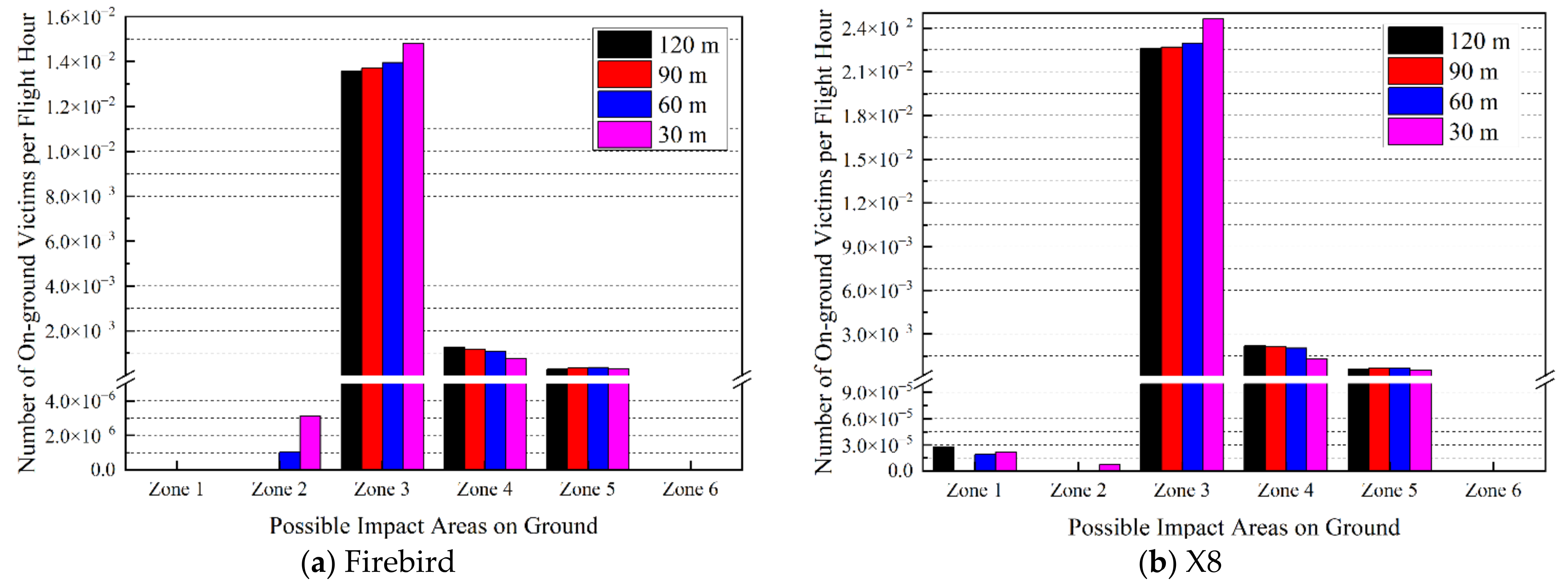
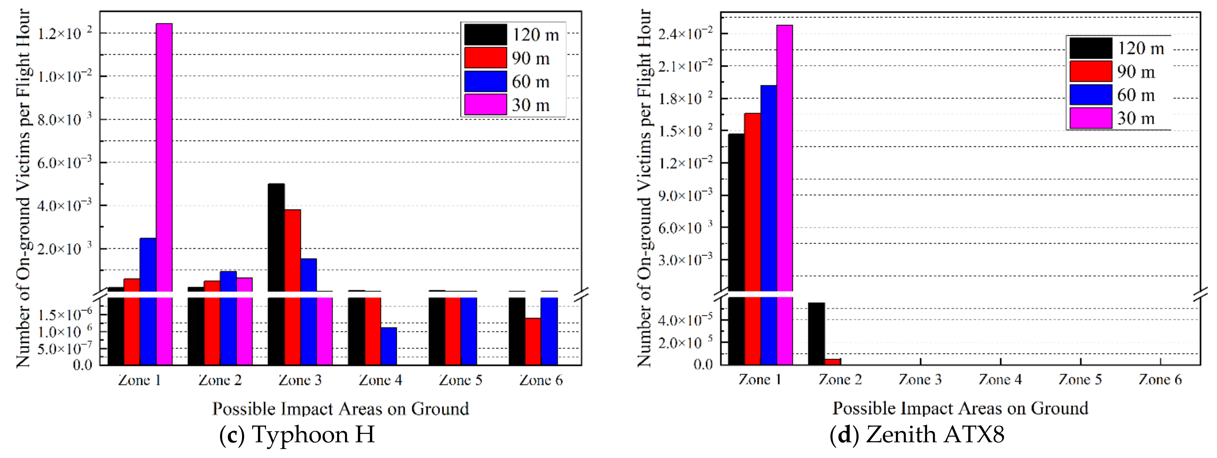
4.5.4. Casualties on the Ground with Different Flying Heights

In this subsection, we mainly consider the effects of flying height on the number of ground victims during the operation of UAVs.

Table 10. Parameters for different flying heights.

Variables	Values
Flying heights	120 m	90 m	60 m	30 m
Wind direction	N (π/2, π/10)
Wind speed	N (3.4, 0.5)
Flight direction	−π/4

gives all the parameters needed for the simulation. It is assumed that all UAVs fail at 120 m, 90 m, 60 m, and 30 m when flying along the same direction of -π/4. Wind effects including speed and direction are also set as stochastic processes with normal distributions of N (3.4, 0.5) and N (π/2, π/10). The detailed results are shown in Figure 13.

In Figure 13a, it can be seen that four zones are affected by Firebird. Out of these, three zones, Zone 3, Zone 4, and Zone 5, are especially notable as each zone shares similar values. The differences in different heights are limited. However, Zone 3 becomes the most dangerous, with 1.48 × 10⁻² ground victims per flight hour. This value is much larger than that in Zone 4 with 1.26 × 10⁻³ and Zone 5 with 3.71 × 10⁻⁴. Zone 2 is safer than the other two. Only when Firebird flies at 60 m and 30 m will Zone 2 be affected by the ground impacts. It is similar for X8 in Zone 3, Zone 4, and Zone 5, as shown in Figure 13b. However, in Zone 2, only the flying height at 30 m leads to ground fatalities for X8. Furthermore, Zone 1 in Figure 13b is affected by X8 when it flies at 120 m, 60 m, and 30 m, with the number of victims being 2.77 × 10⁻⁵, 1.91 × 10⁻⁵, and 2.22 × 10⁻⁵.

In Figure 13c, Typhoon H could crash into every zone with the current flying height settings. The biggest number of victims per flight hour appears in Zone 1 with an altitude of 30 m, which is 1.24 × 10⁻². The smallest is in Zone 4, which is 1.11 × 10⁻⁶ at the height of 60 m. In Figure 13c, Zone 4, Zone 5, and Zone 6 are safe enough that no crash would happen when the flying height is set as 30 m. Zenith ATX8 can only crash into Zone 1 and Zone 2, as given in Figure 13d. Zone 1 is the most dangerous at all flying heights. The corresponding numbers of victims per flight hour are 1.47 × 10⁻², 1.66 × 10⁻², 1.92 × 10⁻², and 2.48 × 10⁻², which increases as the flying height becomes lower. In Zone 2, only the altitude is set as 120 m and 90 m, where a crash could happen for Zenith ATX8, whose values are 5.53 × 10⁻⁵ and 5.16 × 10⁻⁶. The other four zones would not be influenced by Zenith ATX8 under the current settings.

5. Conclusions

In this paper, a ground safety assessment algorithm is proposed to consider the failure of a UAV in the air. The probability of impact positions on the ground being associated with a major in-flight incident is estimated using a second-order drag model and by making probabilistic assumptions regarding the least well-known parameters of the flight. Random factors with multi-uncertainties are dealt with, including uncertainty in drag force, uncertainty in the UAV’s velocity when an event happens, and the random effects of local wind. Then, an effective approach for modeling and estimating the ground risks is presented, in which the number of victims per flight hour caused by the UAV crash is set as the safety index to evaluate the hazards and threats. In the designed multi-factor risk estimation model, ground casualty areas covered by the UAV debris can be calculated based on the parameters of the descending process and characteristics of human beings. In the model, the probability of fatal injuries to people is considered, which is derived by addressing the protection effects provided by ground features, the impact energy of the UAV, and the corresponding energy threshold a person can sustain. Four kinds of sheltering effects are defined to quantize the protection provided by ground features. In order to make the quantization more precise, the areas are partitioned into six zones. The density and distribution of the local population are considered in the proposed algorithm. Official territory and population data of the operation airspace are incorporated, as well as UAV self-properties. Simulations are conducted with actual parameter settings for both fixed-wing and rotary-wing UAVs, in addition to other key elements. The risk levels in different zones on the ground are provided and compared with the widely accepted target safety level of manned aircrafts.

References

1. Clothier, R.A.; Williams, B.P.; Hayhurst, K.J. Modelling the risks remotely piloted aircraft pose to people on the ground. Saf. Sci. 2018, 101, 33–47. [Google Scholar] [CrossRef] [PubMed]
2. Yang, J.; Huang, X. Intelligent Planning Modeling and Optimization of UAV Cluster Based on Multi-Objective Optimization Algorithm. Electronics 2022, 11, 4238. [Google Scholar] [CrossRef]
3. Yang, L.; Zhang, X.; Zhang, Y.; Xiangmin, G. Collision Free 4D Path Planning for Multiple UAVs Based on Spatial Refined Voting Mechanism and PSO Approach. Chin. J. Aeronaut. 2019, 32, 1504–1519. [Google Scholar]
4. Zhang, R.; Dou, L.; Wang, Q.; Xin, B.; Ding, Y. Ability-Restricted Indoor Reconnaissance Task Planning for Multiple UAVs. Electronics 2022, 11, 4227. [Google Scholar] [CrossRef]
5. Clothier, R.A.; Palmer, J.L.; Walker, R.A.; Fulton, N.L. Definition of an airworthiness certification framework for civil unmanned aircraft systems. Saf. Sci. 2011, 49, 871–885. [Google Scholar] [CrossRef]
6. Liu, Y.; Zhang, X.; Guan, X.; Delahaye, D. Potential Odor Intensity Grid Based UAV Path Planning Algorithm with Particle Swarm Optimization Approach. Math. Probl. Eng. 2016, 2016, 7802798. [Google Scholar] [CrossRef]
7. Washington, A.; Clothier, R.A.; Silva, J. A review of unmanned aircraft system ground risk models. Prog. Aerosp. Sci. 2017, 95, 24–44. [Google Scholar] [CrossRef]
8. EASA. Concept of Operations for Drones A Risk Based Approach to Regulation of Unmanned Aircraft; EASA Brochure: Cologne, Germany, 2015. [Google Scholar]
9. Lazatin, J. A Method for Risk Estimation Analysis for Unmanned Aerial System Operation over Populated Areas. In Proceedings of the 14th AIAA Aviation Technology, Integration, and Operations (ATIO) Conference, American Institute of Aeronautics and Astronautics, Atlanta, GA, USA, 16–20 June 2014. [Google Scholar]
10. Lum, C.; Waggoner, B. A Risk Based Paradigm and Model for Unmanned Aerial Systems in the National Airspace. In Proceedings of the Infotech@Aerospace Conferences, American Institute of Aeronautics and Astronautics, Louis, MO, USA, 29–31 March 2011. [Google Scholar]
11. Aalmoes, R.; Cheung, Y.S.; Sunil, E.; Hoekstra, J.M.; Bussink, F. A Conceptual Third Party Risk Model for Personal and Unmanned Aerial Vehicles. In Proceedings of the 2015 International Conference on Unmanned Aircraft Systems (ICUAS), Denver, CO, USA, 9–12 June 2015; pp. 1301–1309. [Google Scholar]
12. Clothier, R.A.; Palmer, J.L.; Walker, R.A.; Fulton, N.L. Definition of Airworthiness Categories for Civil Unmanned Aircraft Systems (UAS). In Proceedings of the 27th International Congress of the Aeronautical Sciences, ICAS, Nice, France, 19–24 September 2010. [Google Scholar]
13. Lum, C.; Gauksheim, K.; Deseure, C.; Vagners, J.; McGeer, T. Assessing and Estimating Risk of Operating Unmanned Aerial Systems in Populated Areas. In Proceedings of the 11th Aviation Technology, Integration, and Operations (ATIO) Conference, American Institute of Aeronautics and Astronautics, Virginia Beach, VA, USA, 20–22 September 2011. [Google Scholar]
14. Ford, A.; McEntee, K. Assessment of the Risk to Ground Population Due to an Unmanned Aircraft In-Flight Failure. In Proceedings of the 10th AIAA Aviation Technology, Integration, and Operations (ATIO) Conference, American Institute of Aeronautics and Astronautics, Fort Worth, TX, USA, 13–15 September 2010. [Google Scholar]
15. Weibel, R.; Hansman, R.J. Safety Considerations for Operation of Different Classes of UAVs in the NAS. In Proceedings of the 4th Aviation Technology, Integration and Operations (ATIO) Conference, American Institute of Aeronautics and Astronautics, Chicago, IL, USA, 20–22 September 2004. [Google Scholar]
16. Burke, D.A.; Hall, C.E.; Cook, S.P. System-Level Airworthiness Tool. J. Aircr. 2011, 48, 777–785. [Google Scholar] [CrossRef]
17. Melnyk, R.; Schrage, D.; Volovoi, V.; Jimenez, H. A Third-Party Casualty Risk Model for Unmanned Aircraft System Operations. Reliab. Eng. Syst. Saf. 2014, 124, 105–116. [Google Scholar] [CrossRef]
18. Courharbo, A.L. Ground impact probability distribution for small unmanned aircraft in ballistic descent. In In Proceedings of the 2020 International Conference on Unmanned Aircraft Systems (ICUAS), Athens, Greece, 1–4 September 2020. [Google Scholar]
19. Courharbo, A.L. Quantifying risk of ground impact fatalities of power line inspection BVLOS flight with small unmanned aircraft. In Proceedings of the 2017 International Conference on Unmanned Aircraft Systems (ICUAS), Miami, FL, USA, 13–16 June 2017; pp. 1352–1360. [Google Scholar]
20. Zhang, X.; Liu, Y.; Zhang, Y.; Guan, X.; Delahaye, D.; Tang, L. Safety Assessment and Risk Estimation for Unmanned Aerial Vehicles Operating in National Airspace System. J. Adv. Transp. 2018, 2018, 4731585. [Google Scholar] [CrossRef]
21. Smith, P.G. Expected Casualty Calculations For Commercial Space Launch and Reentry Missions-Advisory Circular; Technical Report; Federal Aviation Administration: Washington, DC, USA, 2000. [Google Scholar]
22. Dalamagkidis, K.; Valavanis, K.P.; Piegl, L.A. On Integrating Unmanned Aircraft Systems into the National Airspace System: Issues, Challenges, Operational Restrictions, Certification, and Recommendations; Springer Science & Business Media: Berlin/Heidelberg, Germany, 2011. [Google Scholar]
23. Wilde, P. Common Risk Criteria Standards for National Test Ranges; Technical Report; Range Commanders Council: White Sands Missile Range, NM, USA, 2017. [Google Scholar]
24. Guglieri, G.; Quagliotti, F.; Ristorto, G. Operational issues and assessment of risk for light UAVs. J. Unmanned Veh. Syst. 2014, 2, 119–129. [Google Scholar] [CrossRef]
25. Scott, D.W. Kernel Density Estimation. Wiley StatsRef: Statistics Reference Online. 15 February 2018. Available online: https://doi.org/10.1002/9781118445112.stat07186.pub2 (accessed on 18 December 2022). [CrossRef]
26. Botev, Z.I.; Grotowski, J.F.; Kroese, D.P. Kernel Density Estimation via Diffusion. Ann. Stat. 2010, 38, 2916–2957. [Google Scholar] [CrossRef]
27. Chen, Y.C. A Tutorial on Kernel Density Estimation and Recent Advances. Biostat. Epidemiol. 2017, 1, 161–187. [Google Scholar] [CrossRef]
28. Gramacki, A. Nonparametric Kernel Density Estimation and Its Computational Aspects; Springer International Publishing: Cham, Switzerland, 2018. [Google Scholar]
Figure 1. Problem description.
Electronics 12 00829 g001
Figure 2. Casualty area caused by vertical impact.
Electronics 12 00829 g002
Figure 3. Casualty area caused by horizontal impact.
Electronics 12 00829 g003
Figure 4. Simulation scenario.
Electronics 12 00829 g004
Figure 5. Partition of operation area.
Electronics 12 00829 g005
Figure 6. Images of four UAVs used in proposed method.
Electronics 12 00829 g006
Figure 7. Probability estimation of travelled horizontal distance.
Electronics 12 00829 g007aElectronics 12 00829 g007b
Figure 8. Possible ground impact positions with heavy wind.
Electronics 12 00829 g008
Figure 9. Possible ground impact positions with light wind.
Electronics 12 00829 g009
Figure 10. Ground fatalities with different flight directions.
Electronics 12 00829 g010
Figure 11. Ground fatalities with different wind speeds.
Electronics 12 00829 g011
Figure 12. Ground fatalities with different wind directions.
Electronics 12 00829 g012
Figure 13. Ground fatalities with different flying heights.
Electronics 12 00829 g013aElectronics 12 00829 g013b