Optimal Configuration and Scheduling Model of a Multi-Park Integrated Energy System Based on Sustainable Development

Abstract

To maximize the utilization of renewable energy (RE) as much as possible in cold areas while reducing traditional energy use and carbon dioxide emissions, a three-layer configuration optimization and scheduling model considering a multi-park integrated energy system (MPIES), a shared energy storage power station (SESPS), and a hydrogen refueling station (HRS) cooperation based on the Wasserstein generative adversarial networks, the simultaneous backward reduction technique, and the Quantity-Contour (WGAN-SBR_QC) method is proposed. Firstly, the WGAN-SBR_QC method is used to generate typical scenarios of RE output. Secondly, a three-layer configuration and schedule optimization model is constructed using MPIES, SESPS, and HRS. Finally, the model’s validity is investigated by selecting a multi-park in Eastern Mongolia. The results show that: (1) the typical scenario of RE output improved the overall robustness of the system. (2) The profits of the MPIES and HRS increased by 1.84% and 52.68%, respectively, and the SESPS profit increased considerably. (3) The proposed approach increased RE utilization to 99.47% while reducing carbon emissions by 32.67%. Thus, this model is a reference for complex energy system configuration and scheduling, as well as a means of encouraging RE use.

1. Introduction

The collaboration of renewable energy (RE) with energy storage (ES) allows us to accomplish the “dual carbon” target sooner [1]. For some locations rich in RE, collaboration might translate environmental benefits into economic gains. However, RE volatility and the high cost of ES investment are significant variables influencing their development [2]. The emergence of shared energy storage power stations (SESPS) and new energy vehicles, particularly electric vehicles (EV), allows for the suppression of RE instability and the reduction of ES investment costs [3]. However, in cold regions, the usage of EVs is uneconomical [4], and hydrogen fuel vehicles (HFVs) have replaced EVs as the primary equipment. In the 14th Five-year Hydrogen Energy Development Plan of Inner Mongolia Autonomous Region released by the Energy Bureau of Inner Mongolia Autonomous Region in February 2022, 60 hydrogenation stations will be built, and 5000 fuel cell vehicles will be promoted by 2025 [5]. It is clear that the use of HFVs in cold climates has become unavoidable. The cooperation of a multi-park integrated energy system (MPIES), SESPS, and hydrogen refueling station (HRS) in the eastern section of Inner Mongolia is based on plentiful RE. The collaboration of all three will surely alter the output of some units, causing the income of the corresponding main body to decrease or increase. An acceptable and equitable income distribution model is required to boost each participant’s cooperative excitement [6]. Therefore, how to plan equipment, optimize production from the three, and set up an acceptable method of income sharing is critical.

Describing the uncertainty of RE is a prerequisite for developing an optimum allocation and scheduling model. Domestic and foreign scholars have conducted extensive research on the uncertainty of renewable energy, yielding some results. Arman et al. [7], Mei et al. [8], Sneh et al. [9], Liu et al. [10], and Zhao et al. [11] simulated the uncertainties of wind power (WP) and photovoltaic (PV) from the probability distribution curve using Monte Carlo sampling, Latin hypercube sampling, Weibull distribution, Beta distribution, and normal distribution, respectively. Furthermore, Kong et al. [12] and Dahraie et al. [13] adopted the robust random method and the conditional value at risk method, respectively, to represent uncertainty based on uncertainty measurement methodologies. However, the former of these research necessitates precise probability distribution curves, whereas the latter is mathematically too complex. Deep learning algorithms, when compared to existing methods for describing the uncertainty of RE output, can mine the inherent distribution of uncertain variables, address modeling difficulties, and perform unsupervised scene production [14]. In sources [15] and [16], generative adversarial networks (GAN) and Wasserstein generative adversarial networks (WGAN) were used to develop RE production scenarios, and the k-means approach was used to reduce the generated scenarios. However, k-means [17], fuzzy C-means [18], and other clustering algorithms are susceptible to the influence of the initial clustering center and tend to fall into local optimal solutions in the iterative process, and the number of extracted scenes is difficult to determine, therefore the final extracted results are not representative [19]. Yu et al. [20] used a simultaneous backward reduction technique (SBR) based on Quantity-Contour (QC) distance improvement to overcome the clustering challenges above. The WP scenarios created by Yu et al. [20], however, have not been used for planning or dispatching. Hence, the WGAN approach is used in this paper to generate RE scenarios, and the SBR_QC method is used to decrease the scenarios.

In addition, the construction capacity of ES is an essential factor influencing RE usage. However, the high investment cost of ES prevents it from being widely used. Thus, many scholars have researched shared energy storage (SES). Liu et al. [21] presented cloud energy storage as a new SES model and designed operation techniques that considered the interests of cloud energy storage operators and consumers. Wu et al. [22] proposed the SESPS service mode and applied it to MPIES. Based on the literature [22], the capacity and maximum charge–discharge power of SESPS were established as unknown in the literature [23], which were applied to MPIES to drastically minimize SESPS investment, construction, operation, and maintenance expenses. However, the ES investment costs in these studies remain significant. To address this issue, Gao et al. [3] used EV charging stations to help SESPS in serving multiple parks, significantly reducing SESPS capacity. The Gao et al. study, however, does not apply to all scenarios, particularly EVs in cold locations. Furthermore, the construction of HRS offers a novel approach to absorbing more RE [3]. In references [24,25,26], the scheduling of HRS and RE, HRS and microgrid, and HRS and microgrid demand response, and ES were all optimized. All of these studies suggest that HRS play an important role in absorbing RE, but there are few studies on how SESPS and HRS collaborate to serve MPIES, and how their collaboration affects their respective equipment capacity and specific scheduling. Therefore, this paper developed a three-layer configuration optimization and scheduling model of MPIES while considering the collaborative service of SESPS and HRS.

When the studies above are combined, it is discovered that there are still some issues in the configuration and scheduling optimization process of MPIES: (1) the existing scenario generation methods for RE output either require accurate probability distribution curves or are overly complex. None of this is conducive to characterizing renewable energy output. Furthermore, existing RE scene reduction methods are susceptible to the influence of the initial cluster center, and the number of the extracted scenes is difficult to determine, as are the final extracted results. Hence, accurately generating realistic RE output scenarios is an urgent problem. (2) Although ES is thought to be an effective device for absorbing RE, its high investment cost limits its widespread application. The construction of HRS can reduce the capacity construction of ES, but the potential for collaboration between ES, HRS, and multi-park has not been fully realized. In light of the aforementioned issues, this paper proposes a three-layer configuration optimization and scheduling model of the MPIES based on the Wasserstein generative adversarial networks, the simultaneous backward reduction technique, and the Quantity-Contour (WGAN-SBR_QC) method, considering the collaborative service of the SESPS and HRS.

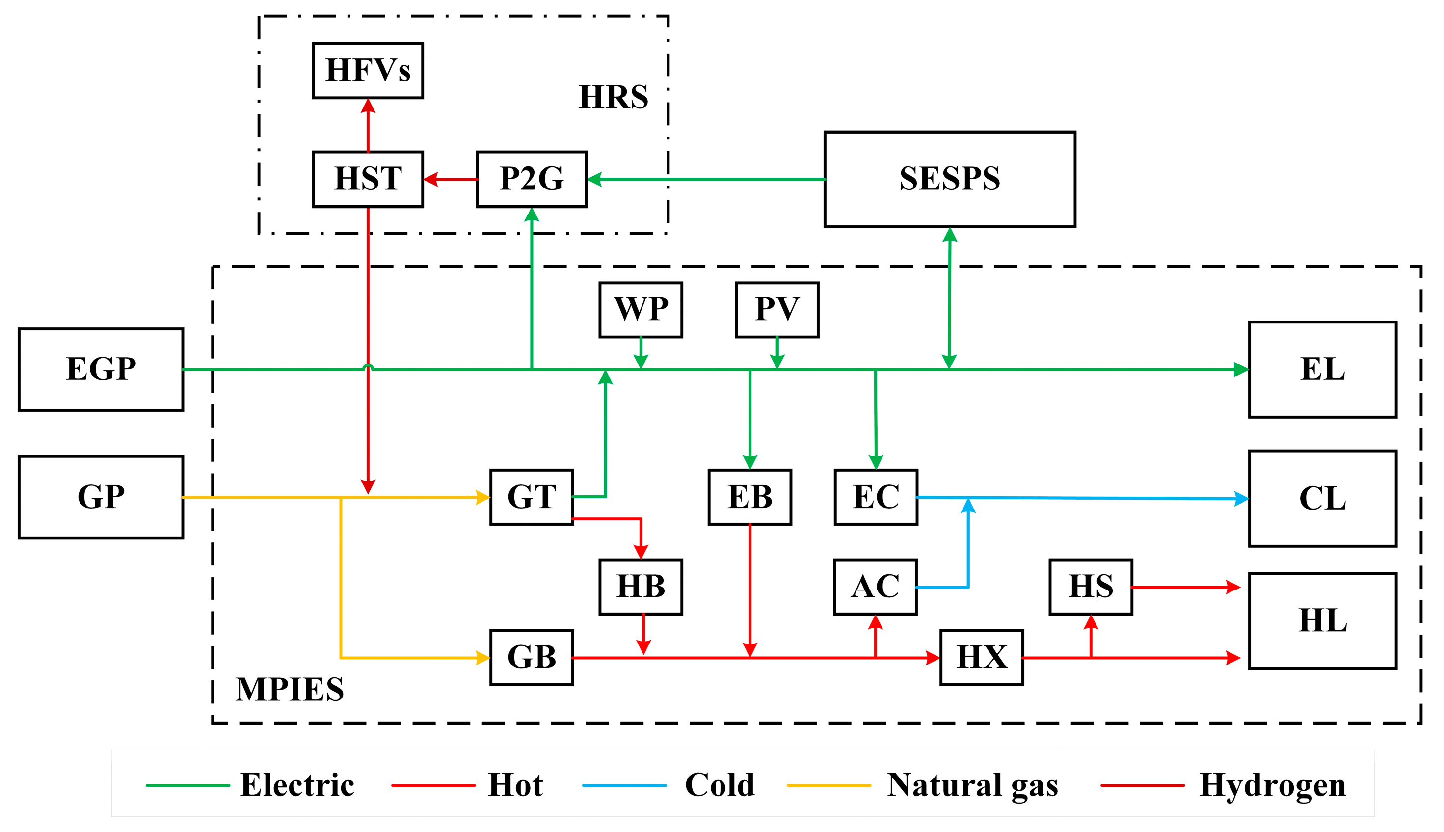
2. The Framework of SESPS and HRS Service

The uncertainty of RE output poses many risks to energy dispatching, and the introduction of ES offers a solution to this challenge. The optimal configuration of SESPS explored in this paper is based on MPIES analysis, and the HRS is applied to it in a novel way. HRS can assist SESPS to absorb a portion of RE while simultaneously providing clean hydrogen (H₂) resources for multi-park and lowering carbon dioxide (CO₂) emissions. Figure 1 depicts the specific structure.

2.1. Service Model

The service mode of SESPS means that the operators of select SESPS locations designed to invest and create large SESPS in MPIES user groups provide ES charging and discharging services for the user groups, operate and manage SESPS, and charge service fees to users. The SESPS service fee is defined as the fee paid by users for charging and discharging per kilowatt-hour of electric energy used with SESPS, expressed in yuan/kWh. Assume the SESPS has no interaction with the grid.

HRS service mode means that HRS operators provide charging and deflating services to HFV and MPIES users, respectively, and are responsible for the operation and management of the HRS, as well as charging consumers related fees, such as fees for charging and servicing for HFV users. The operator also charges MPIES users for a service fee as well as for hydrogen. The corresponding units are $\mathrm{yuan}/\mathrm{kWh}$ and ${\mathrm{yuan}/\mathrm{m}}^3$. To be clear, HRS have their own PV and are recharged by SESPS and MPIES, and surplus hydrogen is acquired from hydrogen-producing plants (suppose a factory produces hydrogen in a conventional way, with CO₂).

The MPIES consumers have three sorts of loads: a cold load (CL), a hot load (HL), and an electric load (EL), all of which are supplied by integrated energy suppliers. The gas turbine (GT), gas boiler (GB), waste heat boiler (WHB), electric boiler (EB), heat exchanger (HX), heat storage (HS), absorption chiller (AC), electric chiller (EC), WP, and PV are the key components of the system. The users’ cooling load demands are met by EC and AC. The HL requirement is met by GB, WHB, EB, HX, and HS. AC is used as heat consumption equipment. PV, WP, and GT power generation in the system prioritizes the power load needs. The EC and EB act as power consumption equipment and insufficient power demand can be obtained from the power grid or SESPS to discharge and supply to consumers. GT and GB are gas consumption devices that are primarily supplied by the external network’s gas plant (GP), with HRS serving as an auxiliary energy supply. The MPIES also buy power from the external grid plant (EGP). The MPIES connected to SESPS and HRS are not allowed to sell electricity to the grid in this paper [23]. If there is excess electric energy in the system, the SESPS or HRS will absorb it through charging or the user will give up the power.

2.2. Operation Mode and Profit Model

SESPS and HRS should follow a priority when providing services to users: the SESPS gives priority to charging and discharging. In the case of overcharging, the HRS provides corresponding charging services to convert electric energy into hydrogen for storage, as described below.

2.2.1. SESPS

Figure 2 depicts an SESPS and HRS diagram. The SESPS establishes an ES control center, and it uses user information, such as the history of grid electricity purchases; cold, hot, and electric load curves; RE output curves; HRS information; and so on, to calculate the SESPS capacity and maximum charge and discharge power based on the user’s needs. The user signs an SESPS service agreement with the SESPS operator based on the calculation findings, which specifies the maximum charge and discharge power, SESPS capacity, charge and discharge power plan required by the user, and charges the service fee to the user. Reference [3] contains specific SESPS and MPIES transactions.

The benefits of SESPS operators stem mostly from three parts: (1) the difference in settlement prices between the user who stores the electric energy in the SESPS and the user who retrieves the electric energy from the SESPS. (2) The SESPS charges users a service fee based on the amount of electric energy transmitted between users and the SESPS. (3) The SESPS charges fees for charging services provided to the HRS.

2.2.2. HRS

The HRS’s operation model and profit model are the same as those of the SESPS, except the discharge service should be converted to a hydrogen discharge service. The priority should be followed. The HRS control center schedules the HFVs depending on the vehicle’s charging status, SESPS supplied information, and other relevant data from the user. The hydrogen storage tank (HST) ensures vehicle inflatable demand. Furthermore, the HRS assists in sharing the configuration of the SESPS to reduce capacity, hence lowering the SESPS investment cost.

3. RE Output Scenarios

3.1. RE Scenarios Generation Based on WGAN

Goodfellow et al. [27] presented GAN as a deep learning model in 2014. It is made up of a generator ($G$) and a discriminator ($D$). Figure 3 depicts the network structure formed by GAN for the scene output.

On the input side of the GAN generator, noise $z$ is the quantity of generator $G$ that generates sample $x^{\prime }=G(z)$. The GAN’s discriminator $D$ must assess the similarity between the produced sample distribution $p(x^{\prime })$ and the actual sample distribution $p(x)$. Thus, (1) and (2) show the loss function of the generator and discriminator in GAN.

$$L_G=-E_{x^{\prime }\sim p(x^{\prime })}\left[D\left(x^{\prime }\right)\right],$$

(1)

$$L_D=-E_{x\sim p(x)}\left[D\left(x\right)\right]+E_{x^{\prime }\sim p(x^{\prime })}\left[D\left(x^{\prime }\right)\right],$$

(2)

where $E$ denotes the expected value of the corresponding distribution. The discriminator function is represented by $D(\sim )$. The real sample is $x$ and the generated sample is $x^{\prime }$.

We need to create another game value function $V(G,D)$ to build the game between the generator $G$ and discriminator $D$ so that they can be educated simultaneously. A minimization game model of value function $V(G,D)$ can be created using (1) and (2), as illustrated in (3):

$$\underset{G}{\min } \underset{D}{\max } V(D,G)=E_{x\sim p(x)}\left[D(x)\right]-E_{x^{\prime }\sim p(x^{\prime })}\left[D(x^{\prime })\right].$$

(3)

Because the loss function of discriminator D in the original GAN is comparable to Jensen–Shannon (JS) divergence [28], it is prone to training issues and mode collapse in training. The JS divergence will be constant if the generated sample does not overlap with the real sample distribution. For RE day-ahead scene creation, the generator must first learn the mapping relationship of the day-ahead scene distribution. If the discriminator employs the JS divergence as the loss function, it will be unable to reliably calculate the distance between the sample distributions, and the gradient will vanish in the reverse transfer. The issue of difficulty in the network training affects the correctness of the generated scene set. Wasserstein distance may efficiently measure and quantify the distance between two probability distributions, even when they do not overlap [29]. The Wasserstein distance is defined as:

$$W(p(x),p(x^{\prime }))=\underset{\pi (x,x^{\prime })}{\inf }{\displaystyle \int d(x,x^{\prime })\pi (dx,d{x}^{\prime })},$$

(4)

where $\pi (x,x^{\prime })$ is the joint probability density distribution meeting the edge distribution of $p(x)$ and $p(x^{\prime })$. $d(x,x^{\prime })$ represents the distance between scenes. Using Wasserstein distance as the discriminator loss function instead of JS divergence can successfully alleviate the problems of training difficulties and mode collapse, while also better fitting the probability distribution [30]. However, the Wasserstein distance is difficult to compute directly, which is similar to solving an optimal transmission issue.

Therefore, in GAN, the Kantorovich–Rubinstein dual form is commonly employed to describe the distance between the generated and real samples. When applied to GAN, it can be written as follows:

$$W_{\left(p_{(x)},p_{(x^{\prime })}\right)}=\underset{{‖f_D‖}_L\le 1}{\sup }{E}_{p(x)}\left[D(x)\right]-E_{p(x^{\prime })}\left[D(x^{\prime })\right],$$

(5)

where ${‖f_D‖}_L\le 1$ is the $1-\mathrm{Lipschitz}$ continuity that the discriminator loss function should meet and the absolute value of its derivative’s upper bound is 1.

To ensure that the discriminator function roughly fulfills the $1-\mathrm{Lipschitz}$ continuity, the gradient penalty function of function $D$ in the domain can be inserted into (3), such that the discriminator loss function can properly describe the Wasserstein distance. Hence, the GAN objective function may be transformed into [31]:

$$\underset{G}{\min } \underset{D}{\max } V(D,G)=E_{x\sim p(x)}\left[D(x)\right]-E_{x^{\prime }\sim p(x^{\prime })}\left[D(x^{\prime })\right]-\lambda E{\left[‖\nabla D(\sim )‖-1\right]}^2,$$

(6)

where $\lambda E{\left[‖\nabla D(\sim )‖-1\right]}^2$ is the penalty function of the discriminator $D$’s loss function gradient and $\lambda$ is the penalty coefficient.

3.2. RE’s Scene Cuts

The trained WGAN is used to generate $N$ windspeed and $N$ solar radiation intensity situations, yielding a set of $N^2$ scenarios in total. The scenario set grows exponentially as $N$ increases, resulting in significant computing complexity. As a result, the number of scenarios must be lowered in order to reduce the quantity of calculation. To lower the output of RE, the simultaneous backward reduction algorithm based on quantity-contour distance (SBR_QC) in reference [20] is utilized (using the WP output as an example).

The initial scene set of $N$ days windspeed is $X={\left[X_1,X_2,\cdots ,X_N\right]}^{\prime }$, with the $i(i=1,2,\cdots ,N)$ scene being $X_i=\left[x_{i1},x_{i2},\cdots ,x_{iT}\right]$, the sampling time node being $t(t=1,2,\cdots ,T)$, the corresponding probability of the initial scene being $X_i=\left[x_{i1},x_{i2},\cdots ,x_{iT}\right]$, the extracted scene number being $M$, the deleted scene set being $Y$, the scene number contained in $Y$ being $(N-M)$, and the final scene set being $(X-Y)$. Set $X_i,X_j\in X$, initially delete scene set $Y^0=\varphi$, and then proceed as follows:

(1)

Calculate the QC distance between each two scenes in the initial scene set using (7).

$$d\left(X_i,X_j\right)={\displaystyle \sum _{t=1}^T\left|x_{it}-x_{jt}\right|}\times {\displaystyle \sum _{t=1}^T\left|{\theta }_{it}-{\theta }_{jt}\right|}+\left[\left(\max X_i-\min X_i\right)-\left(\max X_j-\min X_j\right)\right],$$

(7)

where $\max X_i$, $\min X_i$, $\max X_j$, and $\min X_j$ represent the maximum and minimum windspeeds in scenes $X_i$ and $X_j$. ${\theta }_{it}$ reflects the shape dimension fluctuation of the WP output scenario $i$ at $t$. The scenario probability can be found in reference [20].

(2)

The $k(k=1,2,\cdots ,(N-M))$ reduction results in:

$$\left\{\begin{array}{l}{d}_{lj}^k=\underset{X_j\notin Y^{k-1}\cup \left\{X_l^k\right\}}{\min }d\left(X_l,X_j\right)\\ D_{lj}^k=P_l\times d_{lj}^k\end{array}\right. X_l\notin Y^{k-1} .$$

(8)

To obtain $Y^k=Y^{k-1}\cup \left\{X_l^k\right\}$, the scene $X_l^k$ corresponding to the smallest $D_{lj}^k$ is eliminated from the scene set $\left(X-Y^{k-1}\right)$ and integrated into the deleted scene $Y^{k-1}$. The probability relating to scene $X_l^k$ is added to the probability $P_j^{k-1}$ corresponding to scene $X_j^{k-1}$ closest to scene $X_l^k$ in scene set $\left(X-Y^{k-1}\right)$. In the updated scene set $\left(X-Y^k\right)$, the distance between each two scene combinations is determined afresh.

(3)

The more similar the two scenarios are, the more likely they are to be categorized in the same category. The intra-class similarity $S(M)$ is defined to quantify the intra-class similarity of various sorts of situations. $(N-M)$ is determined based on the number of deleted scenes, including the usual scene set $X^C$ of $M$ class situations and the likelihood of typical scene occurrence $P^C$. Meanwhile, $Z^{(m)}$ focused on $X_m^C(m=1,2,\cdots ,M)$ is recorded, where:

$$X^C={\left[X_1^C,X_2^C,\cdots X_M^C\right]}^{\prime }=\left(\begin{array}{cccc}{x}_{1,1}^C& x_{1,2}^C& \cdots & x_{1,T}^C\\ x_{2,1}^C& x_{2,2}^C& \cdots & x_{2,T}^C\\ ⋮& ⋮& ⋮& ⋮\\ x_{M,1}^C& x_{M,2}^C& \cdots & x_{M,T}^C\end{array}\right),$$

(9)

$$P^C={\left[P_1^C,P_2^C,\cdots ,P_M^C\right]}^{\prime },$$

(10)

$$Z^{(m)}={\left[X_1^{(m)},X_2^{(m)},\cdots ,X_{N_m}^{(m)}\right]}^{\prime }=\left(\begin{array}{cccc}{x}_{1,1}^{(m)}& x_{1,2}^{(m)}& \cdots & x_{1,T}^{(m)}\\ ⋮& ⋮& ⋮& ⋮\\ x_{N_m-1,1}^{(m)}& x_{N_m-1,2}^{(m)}& \cdots & x_{N_m-1,T}^{(m)}\\ x_{N_m,1}^{(m)}& x_{N_m,2}^{(m)}& \cdots & x_{N_m,T}^{(m)}\end{array}\right),$$

(11)

where $X_m^C$ represents the $m$ class scene in the typical scene set. $P_m^C$ represents the probability of occurrence of a type $m$ scene in the typical scene set, $P_1^C+P_2^C+\cdots +P_M^C=1$. $N_m$ represents the number of scenarios in category $m$ except $X_m^C$, ${\displaystyle \sum _{m=1}^M{N}_m}=N-M$; $X_{N_m}^{(m)}$ represents the $N_m$th scenario to be incorporated into scenario $X_m^C$.

Calculate the intra-class similarity $S(M)$:

$$S(M)={\displaystyle \sum _{m=1}^M\frac{P_m^{C}d\left(X_m^C,Z^{(m)}\right)}{N_m}},$$

(12)

where $d\left(X_m^C,Z^{(m)}\right)$ denotes the distance between all scenes in scene sets $Z^{(m)}$ and $X_m^C$. The mean probability distance between each scene in $Z^{(m)}$ and $X_m^C$ is represented by $\frac{P_m^{C}d\left(X_m^C,Z^{(m)}\right)}{N_m}$. $S(M)$ is the probability average intra-class distance of $M$ scenarios, which fully captures the intra-class similarity of $M$ scenarios. The lower the $S(M)$, the higher the intra-class similarity of $M$ scenarios and the more ideal the scene reduction impact.

(4)

The greater the contrast between the two scenes, the easier it is to categorize them. The difference degree $D(M)$ between classes is defined to assess the difference between different sorts of scenarios. Two scenes, $X_u^C$ and $X_v^C$$\left(u,v=1,2,\cdots ,M\right)$, are chosen at random from scene set $X^C$ for a total of $n\left(C_M^2\right)$ combination modes. Any two scenes’ similarity distance is calculated as follows:

$$d\left(X_u^C,X_v^C\right)=\left\{\begin{array}{ll}d\left(X_u^C,X_v^C\right), & u\ne v\\ 0,& u=v\end{array}\right..$$

(13)

Calculate the inter-class difference degree $D(M)$ between class $M$ scenarios:

$$D(M)=\frac{{\displaystyle \sum _{u=1}^M{\displaystyle \sum _{v=1}^{M}d\left(X_u^C,X_v^C\right)}}}{2\times n\left(C_M^2\right)}.$$

(14)

As the scenes reduce further, similar sequences are repeatedly merged, and the variations between the remaining scenes become increasingly pronounced. To quantify the differences between the remaining scenarios, the inter-class difference degree $D(M)$ is used. The bigger the similarity gap between the remaining scenes, the greater the disparity between the various scenarios in the reduced scene set $X^C$.

(5)

Calculate the scenario reduction validity index.

Scenario reduction ($SD$) is composed of intra-class similarity and inter-class difference, with the following calculation formula:

$$SD\left(M\right)=\frac{S(M)}{D(M)}.$$

(15)

The number of distinct scenes $M$ correlates to various $SD$ index values. The smaller the intra-class similarity $S(M)$, the larger the inter-class difference $D(M)$, and the smaller the $SD$ index value, the greater the degree of difference across $M$ scenes achieved. The $SD$ index reduction is greatest when the corresponding number of scenarios is considered to be the best scenario for the $M$. However, when the number of scenarios is larger, if the scenarios are set in scenarios with an extraction probability less than 5% (that is, scenarios with low probability), the probability of various scenarios is smaller, indicating that the scenarios are not conducive to actual analysis. Assuming no low-probability scenario exists, the number of scenes corresponding to the first fall in the $SD$ index value or the first inflection point can be regarded as the final extraction number of scenes.

(6)

Because it is a large time scale configuration problem, typical WP and PV scenarios from different seasons are mixed, as illustrated in (16).

$$\left\{\begin{array}{l}{v}_{\mathrm{WT}}={\displaystyle \sum _{m=1}^M{X}_{\mathrm{WT},m}^C\cdot P_{\mathrm{WT},m}^C}\\ f_{\mathrm{PV}}={\displaystyle \sum _{m=1}^M{X}_{\mathrm{PV},m}^C\cdot P_{\mathrm{PV},m}^C}\end{array}\right..$$

(16)

3.3. RE Output

The output of RE is calculated using (17)–(18) [3].

$$P_{\mathrm{WT}}(t)=\left\{\begin{array}{ll}0& v_{\mathrm{WT}}(t)\le v_{\mathrm{in}}\\ \frac{v_{\mathrm{WT}}(t)-v_{\mathrm{in}}}{v_{\mathrm{R}}-v_{\mathrm{in}}}\cdot P_{\mathrm{WT},\mathrm{R}}& v_{\mathrm{in}}<v_{\mathrm{WT}}(t)\le v_{\mathrm{R}}\\ P_{\mathrm{WT},\mathrm{R}}& v_{\mathrm{R}}<v_{\mathrm{WT}}(t)\le v_{\mathrm{out}}\\ 0& v_{\mathrm{WT}}(t)>v_{\mathrm{out}}\end{array}\right.,$$

(17)

$$P_{\mathrm{PV}}(t)={\eta }_{\mathrm{PV}}\cdot S_{\mathrm{PV}}\cdot f_{\mathrm{PV}}(t).$$

(18)

4. Three-Layer Configuration Optimization Model

The MPIESs layer, SESPS layer, and HRS layer comprise the three-layer configuration optimization model. Figure 4 depicts the specifics.

4.1. MPIESs Layer: Equipment Planning and Optimization Operation

The MPIESs layer is primarily used to solve equipment planning and output issues.

4.1.1. Objective Function

The MPIESs layer’s objective function is to maximize the annual net profit, as shown below:

$$\max F_{\mathrm{mp}}={\displaystyle \sum _{w=1}^W{D}_w\cdot \left(\begin{array}{l}\tau R_{\mathrm{mp-sesps},\mathrm{s}}^w+\theta R_{\mathrm{mp-hrs},\mathrm{s}}^w-C_{\mathrm{mp-grid}}^w-C_{\mathrm{mp}\_\mathrm{fuel}}^w-\tau C_{\mathrm{mp-sesps},\mathrm{b}}^w\\ -\theta C_{\mathrm{mp-hrs},\mathrm{b}}^w-\tau C_{\mathrm{mp-sesps}\_\mathrm{serve}}^w-\theta C_{\mathrm{mp-hrs}\_\mathrm{serve}}^w-C_{\mathrm{mp}\_\mathrm{inv}}^w\end{array}\right)}.$$

(19)

(1)

Revenue from electricity sales to SESPS:

$$R_{\mathrm{mp-sesps},\mathrm{s}}^w={\displaystyle \sum _{i=1}^I{\displaystyle \sum _{t=1}^T{p}_{\mathrm{mp-sesps},\mathrm{s}}(t)\cdot P_{\mathrm{mp-sesps},\mathrm{s}}^{w,i}(t)\cdot \Delta t\cdot U_{\mathrm{mp-sesps},\mathrm{s}}^{w,i}(t)}}$$

(20)

(2)

Revenue from electricity sales to HRS:

$$R_{\mathrm{mp-hrs},\mathrm{s}}^w={\displaystyle \sum _{i=1}^I{\displaystyle \sum _{t=1}^T{p}_{\mathrm{mp-hrs},\mathrm{s}}(t)\cdot P_{\mathrm{mp-hrs},\mathrm{s}}^{w,i}(t)\cdot \Delta t\cdot U_{\mathrm{mp-hrs},\mathrm{s}}^{w,i}(t)}}$$

(21)

(3)

The cost of buying electricity from the grid:

$$C_{\mathrm{mp-grid}}^w={\displaystyle \sum _{i=1}^I{\displaystyle \sum _{t=1}^T{p}_{\mathrm{mp-grid}}(t)\cdot P_{\mathrm{mp-grid}}^{w,i}(t)\cdot \Delta t}}$$

(22)

(4)

The cost of buying gas from the external grid:

$$C_{\mathrm{mp}\_\mathrm{fuel}}^w={\displaystyle \sum _{i=1}^I{\displaystyle \sum _{t=1}^T{c}_{\mathrm{gas}}\left(\frac{P_{\mathrm{GT}}^{w,i}(t)}{{\eta }_{\mathrm{GT}}H{n}_{\mathrm{NG}}}+\frac{H_{\mathrm{GB}}^{w,i}(t)}{{\eta }_{\mathrm{GB}}H{n}_{\mathrm{NG}}}-V_{\mathrm{mp-hrs},\mathrm{cq}}^{w,i}(t)\cdot {\eta }_{{\mathrm{h}}_2}\right)}}$$

(23)

(5)

The cost of buying electricity from SESPS:

$$C_{\mathrm{mp-sesps},\mathrm{b}}^w={\displaystyle \sum _{i=1}^I{\displaystyle \sum _{t=1}^T{p}_{\mathrm{mp-sesps},\mathrm{b}}(t)\cdot P_{\mathrm{mp-sesps},\mathrm{b}}^{w,i}(t)\cdot \Delta t\cdot U_{\mathrm{mp-sesps},\mathrm{b}}^w(t)}}$$

(24)

(6)

The cost of buying hydrogen from HRS:

$$C_{\mathrm{mp-hrs},\mathrm{b}}^w={\displaystyle \sum _{i=1}^I{\displaystyle \sum _{t=1}^T{p}_{\mathrm{mp-hrs},\mathrm{b}}(t)\cdot V_{\mathrm{mp-hrs},\mathrm{b}}^{w,i}(t)\cdot U_{\mathrm{mp-hrs},\mathrm{b}}^w(t)}}$$

(25)

(7)

The cost of service fees from SESPS:

$$C_{\mathrm{mp-sesps}\_\mathrm{serve}}^w={\displaystyle \sum _{i=1}^I{\displaystyle \sum _{t=1}^T{p}_{\mathrm{mp-sesps}\_\mathrm{serve}}(t)\cdot \left(\begin{array}{l}{P}_{\mathrm{mp-sesps},\mathrm{b}}^{w,i}(t)\cdot U_{\mathrm{mp-sesps},\mathrm{b}}^w(t)\\ +P_{\mathrm{mp-sesps},\mathrm{s}}^{w,i}(t)\cdot U_{\mathrm{mp-sesps},\mathrm{s}}^w(t)\end{array}\right)\cdot \Delta t}}$$

(26)

(8)

The cost of service fees from HRS:

$$C_{\mathrm{mp-hrs}\_\mathrm{serve}}^w={\displaystyle \sum _{i=1}^I{\displaystyle \sum _{t=1}^T\left(\begin{array}{l}{p}_{\mathrm{mp-hrs}\_\mathrm{ch}\_\mathrm{serve}}(t)\cdot P_{\mathrm{mp-hrs},\mathrm{s}}^{w,i}(t)\cdot \Delta t\cdot U_{\mathrm{mp-hrs},\mathrm{s}}^w(t)\\ +p_{\mathrm{mp-hrs}\_\mathrm{fq}\_\mathrm{serve}}(t)\cdot V_{\mathrm{mp-hrs},\mathrm{b}}^{w,i}(t)\cdot U_{\mathrm{mp-hrs},\mathrm{b}}^w(t)\end{array}\right)}}$$

(27)

(9)

The cost of the MPIES’s average daily investment and maintenance:

$$C_{\mathrm{mp}\_\mathrm{inv}}^w={\displaystyle \sum _{j=1}^J\left(\frac{C_{\mathrm{equ}\_\mathrm{inv}}^j}{D_{\mathrm{equ}}^j}+C_{\mathrm{equ}\_\mathrm{main}}^j\right)}$$

(28)

4.1.2. Constraints of the MPIES

The MPIES’ constraints for a typical day are as follows.

(1)

Electrical power balance:

$$\begin{array}{l}{P}_{\mathrm{GT}}^{w,i}(t)+P_{\mathrm{WT}}^{w,i}(t)+P_{\mathrm{PV}}^{w,i}(t)+P_{\mathrm{mp-grid}}^{w,i}(t)+\tau P_{\mathrm{mp-sesps},\mathrm{b}}^{w,i}(t)-\tau P_{\mathrm{mp-sesps},\mathrm{s}}^{w,i}(t)\\ -\theta P_{\mathrm{mp-hrs},\mathrm{s}}^{w,i}(t)-P_{\mathrm{EC}}^{w,i}(t)-P_{\mathrm{EB}}^{w,i}(t)-P_{\mathrm{load}}^{w,i}(t)=0\end{array}$$

(29)

(2)

Cold power balance:

$$P_{\mathrm{EC}}^{w,i}(t)\cdot CO{P}_{\mathrm{EC}}+Q_{\mathrm{AC}}^{w,i}(t)-Q_{\mathrm{load}}^{w,i}(t)=0$$

(30)

(3)

Hot power balance:

$$H_{\mathrm{HX}}^{w,i}(t)+H_{\mathrm{EB}}^{w,i}(t)+H_{\mathrm{HS},\mathrm{dis}}^{w,i}(t)-H_{\mathrm{HS},\mathrm{ch}}^{w,i}(t)-H_{\mathrm{load}}^{w,i}(t)=0$$

(31)

(4)

Hydrogen balance:

$$0\le V_{\mathrm{mp-hrs},\mathrm{cq}}^{w,i}(t)\le V_{\mathrm{mp-hrs},\mathrm{cq}}^{\max }$$

(32)

(5)

HB’s waste heat balance:

$$\left\{\begin{array}{l}\frac{H_{\mathrm{HX}}^{w,i}(t)}{{\eta }_{\mathrm{HX}}}+\frac{Q_{\mathrm{AC}}^{w,i}(t)}{CO{P}_{\mathrm{AC}}}-H_{\mathrm{HB}}^{w,i}(t)-H_{\mathrm{GB}}^{w,i}(t)-H_{\mathrm{EB}}^{w,i}(t)=0\\ H_{\mathrm{HB}}^{w,i}(t)=P_{\mathrm{GT}}^{w,i}(t){\gamma }_{GT}{\eta }_{\mathrm{HB}}\end{array}\right.$$

(33)

(6)

HS balance:

$$S_{\mathrm{hs}}^{w,i}(t)=(1-{\eta }_{\mathrm{hs},\mathrm{loss}})S_{\mathrm{hs}}^{w,i}(t-1)+\left({\eta }_{\mathrm{hs},\mathrm{ch}}{H}_{\mathrm{hs},\mathrm{ch}}^{w,i}(t)\cdot U_{\mathrm{sesps-mp},\mathrm{ch}}^w(t)-\frac{H_{\mathrm{hs},\mathrm{dis}}^{w,i}(t)\cdot U_{\mathrm{hs},\mathrm{dis}}^{w,i}(t)}{{\eta }_{\mathrm{hs},\mathrm{dis}}}\right)\Delta t/S_{\mathrm{hs}},$$

(34)

$$\left\{\begin{array}{l}{S}_{\mathrm{hs}}^{w,i}(0)=S_{\mathrm{hs}}^{w,i}(24)=0.5(S_{\mathrm{hs}}^{\max }+S_{\mathrm{hs}}^{\min })\\ S_{\mathrm{hs}}^{\min }\le S_{\mathrm{hs}}^{w,i}(t)\le S_{\mathrm{hs}}^{\max }\\ 0\le H_{\mathrm{hs},\mathrm{ch}}^{w,i}(t)\le H_{\mathrm{hs},\mathrm{ch}}^{\max }\\ 0\le H_{\mathrm{hs},\mathrm{dis}}^{w,i}(t)\le H_{\mathrm{hs},\mathrm{dis}}^{\max }\\ U_{\mathrm{hs},\mathrm{ch}}^{w,i}(t)+U_{\mathrm{hs},\mathrm{dis}}^{w,i}(t)\le 1\\ U_{\mathrm{hs},\mathrm{ch}}^{w,i}(t)\in \left\{0,1\right\},U_{\mathrm{hs},\mathrm{dis}}^{w,i}(t)\in \left\{0,1\right\}\end{array}\right..$$

(35)

(7)

SESPS’s charging and discharging power balance.

The SESPS charge and discharge power is the sum of the power purchased and sold by the MPIES and the SESPS.

$${\displaystyle \sum _{i=1}^I\left(P_{\mathrm{mp-sesps},\mathrm{s}}^{w,i}(t)-P_{\mathrm{mp-sesps},\mathrm{b}}^{w,i}(t)\right)}=P_{\mathrm{sesps-mp},\mathrm{ch}}^w(t)-P_{\mathrm{sesps-mp},\mathrm{dis}}^w(t)$$

(36)

(8)

Equipment output:

$$\left\{\begin{array}{l}{P}_{\mathrm{equ}}^{\min }{U}_{\mathrm{equ}}^{\mathrm{inv},i}\le P_{\mathrm{equ}}^{w,i}(t)\le P_{\mathrm{equ}}^{\max }{U}_{\mathrm{equ}}^{\mathrm{inv},i}\\ U_{\mathrm{equ}}^{\mathrm{inv},i}\in \left\{0,1\right\}\end{array}\right.$$

(37)

(9)

The grid’s power purchase constraint:

$$0\le P_{\mathrm{mp-grid}}^{w,i}(t)\le P_{\mathrm{mp-grid}}^{\max }$$

(38)

(10)

Power constraints between MPIES and SESPS:

$$\left\{\begin{array}{l}0\le P_{\mathrm{mp-sesps},\mathrm{s}}^{w,i}(t)\le P_{\mathrm{mp-sesps}}^{\max }\\ 0\le P_{\mathrm{mp-sesps},\mathrm{b}}^{w,i}(t)\le P_{\mathrm{mp-sesps}}^{\max }\\ U_{\mathrm{mp-sesps},\mathrm{s}}^{w,i}(t)+U_{\mathrm{mp-sesps},\mathrm{b}}^{w,i}(t)\le 1\\ U_{\mathrm{mp-sesps},\mathrm{s}}^{w,i}(t)\in \left\{0,1\right\},U_{\mathrm{mp-sesps},\mathrm{b}}^{w,i}(t)\in \left\{0,1\right\}\end{array}\right.$$

(39)

(11)

Power constraints between MPIES and HRS:

$$\left\{\begin{array}{l}0\le P_{\mathrm{mp-hrs},\mathrm{s}}^{w,i}(t)\le P_{\mathrm{mp-hrs}}^{\max }\\ 0\le V_{\mathrm{mp-hrs},\mathrm{b}}^{w,i}(t)\le V_{\mathrm{mp-hrs}}^{\max }\\ U_{\mathrm{mp-hrs},\mathrm{s}}^{w,i}(t)+U_{\mathrm{mp-hrs},\mathrm{b}}^{w,i}(t)\le 1\\ U_{\mathrm{mp-hrs},\mathrm{s}}^{w,i}(t)\in \left\{0,1\right\},U_{\mathrm{mp-hrs},\mathrm{b}}^{w,i}(t)\in \left\{0,1\right\}\end{array}\right.$$

(40)

(12)

Constraints of RE:

$$\left\{\begin{array}{l}0\le P_{\mathrm{WT}}^{w,i}(t)\le P_{\mathrm{WT-G}}^{w,i}(t)\\ 0\le P_{\mathrm{PV}}^{w,i}(t)\le P_{\mathrm{PV-G}}^{w,i}(t)\end{array}\right.$$

(41)

4.2. SESPS Layer: Planning Optimization

The decision variables for determining the optimal annual profit of the SESPS during the planning period include capacity allocation and the SESPS’s maximum charge and discharge power.

4.2.1. Objective Function

As the objective function, the maximum annual SESPS profit is shown in (42):

$$\max F_{\mathrm{sesps}}={\displaystyle \sum _{w=1}^W{D}_w\left(\begin{array}{l}\tau R_{\mathrm{sesps-mp},\mathrm{dis}}^w+\delta R_{\mathrm{sesps-hrs},\mathrm{dis}}^w+\tau R_{\mathrm{sesps-mp}\_\mathrm{serve}}^w+\delta R_{\mathrm{sesps-hrs}\_\mathrm{serve}}^w\\ -C_{\mathrm{inv}}^w-\tau C_{\mathrm{sesps-mp},\mathrm{ch}}^w-\delta C_{\mathrm{sesps-hrs},\mathrm{ch}}^w\end{array}\right)}$$

(42)

(1)

Revenue from selling electricity to MPIES:

$$R_{\mathrm{sesps-mp},\mathrm{dis}}^w={\displaystyle \sum _{i=1}^I{\displaystyle \sum _{t=1}^T{p}_{\mathrm{sesps-mp},\mathrm{dis}}(t)\cdot P_{\mathrm{sesps-mp},\mathrm{dis}}^{w,i}(t)\cdot \Delta t\cdot U_{\mathrm{sesps-mp},\mathrm{dis}}^w(t)}}$$

(43)

(2)

Revenue from selling electricity to HRS:

$$R_{\mathrm{sesps-hrs},\mathrm{dis}}^w={\displaystyle \sum _{j=1}^J{\displaystyle \sum _{t=1}^T{p}_{\mathrm{sesps-hrs},\mathrm{dis}}(t)\cdot P_{\mathrm{sesps-hrs},\mathrm{dis}}^{w,j}(t)\cdot \Delta t\cdot U_{\mathrm{sesps-hrs},\mathrm{dis}}^w(t)}}$$

(44)

(3)

Revenue of service charge from MPIES:

$$R_{\mathrm{sesps-mp}\_\mathrm{serve}}^w={\displaystyle \sum _{i=1}^I{\displaystyle \sum _{t=1}^T{p}_{\mathrm{sesps-mp}\_\mathrm{serve}}(t)\cdot \left(\begin{array}{l}{P}_{\mathrm{sesps-mp},\mathrm{dis}}^{w,i}(t)\cdot U_{\mathrm{sesps-mp},\mathrm{dis}}^w(t)\\ +P_{\mathrm{sesps-mp},\mathrm{ch}}^{w,i}(t)\cdot U_{\mathrm{sesps-mp},\mathrm{ch}}^w(t)\end{array}\right)\cdot \Delta t}}$$

(45)

(4)

Revenue of service charge from HRS:

$$R_{\mathrm{sesps-hrs}\_\mathrm{serve}}^w={\displaystyle \sum _{i=1}^I{\displaystyle \sum _{t=1}^T{p}_{\mathrm{sesps-hrs}\_\mathrm{serve}}(t)\cdot \left(\begin{array}{l}{P}_{\mathrm{sesps-hrs},\mathrm{dis}}^{w,i}(t)\cdot U_{\mathrm{sesps-hrs},\mathrm{dis}}^w(t)\\ +P_{\mathrm{sesps-hrs},\mathrm{ch}}^{w,i}(t)\cdot U_{\mathrm{sesps-hrs},\mathrm{ch}}^w(t)\end{array}\right)\cdot \Delta t}}$$

(46)

(5)

The cost of SESPS average daily investment and maintenance [23]:

$$C_{\mathrm{inv}}^w=\frac{p_{P_{\mathrm{sesps}}}\cdot P_{\mathrm{sesps}}^{\max }+p_{S_{\mathrm{sesps}}}\cdot S_{\mathrm{sesps}}^{\max }}{D_{\mathrm{sesps}}}+C_{\mathrm{sesps-main}}$$

(47)

(6)

The cost of purchasing electricity from MPIES:

$$C_{\mathrm{sesps-mp},\mathrm{ch}}^w={\displaystyle \sum _{i=1}^I{\displaystyle \sum _{t=1}^T{p}_{\mathrm{sesps-mp},\mathrm{ch}}(t)\cdot P_{\mathrm{sesps-mp},\mathrm{ch}}^{w,i}(t)\cdot \Delta t\cdot U_{\mathrm{sesps-mp},\mathrm{ch}}^w(t)}}$$

(48)

(7)

The cost of purchasing electricity from HRS:

$$C_{\mathrm{sesps-hrs},\mathrm{ch}}^w={\displaystyle \sum _{i=1}^I{\displaystyle \sum _{t=1}^T{p}_{\mathrm{sesps-hrs},\mathrm{ch}}(t)\cdot P_{\mathrm{sesps-hrs},\mathrm{ch}}^{w,i}(t)\cdot \Delta t\cdot U_{\mathrm{sesps-hrs},\mathrm{ch}}^w(t)}}$$

(49)

4.2.2. Constraints of the SESPS

(1)

Scaling constraints of SESPS.

The SESPS capacity is proportional to the rated power [23], as shown below:

$$S_{\mathrm{sesps}}^{\max }=\beta \cdot P_{\mathrm{sesps}}^{\max }\cdot \Delta t$$

(50)

(2)

SESPS’s charge and discharge power constraints:

$$S_{\mathrm{sesps}}^w(t)=(1-{\eta }_{\mathrm{sesps},\mathrm{loss}})S_{\mathrm{sesps}}^w(t-1)+\left(\begin{array}{l}{\eta }_{\mathrm{sesps},\mathrm{ch}}\tau P_{\mathrm{sesps-mp},\mathrm{ch}}^w(t)\cdot U_{\mathrm{sesps-mp},\mathrm{ch}}^w(t)\\ -\frac{\tau P_{\mathrm{sesps-mp},\mathrm{dis}}^w(t)\cdot U_{\mathrm{sesps-mp},\mathrm{dis}}^w(t)+\theta P_{\mathrm{sesps-hrs},\mathrm{dis}}^w(t)\cdot U_{\mathrm{sesps-hrs},\mathrm{dis}}^w(t)}{{\eta }_{\mathrm{sesps},\mathrm{dis}}}\end{array}\right)\Delta t/S_{\mathrm{sesps}}^{},$$

(51)

$$\left\{\begin{array}{l}{S}_{\mathrm{sesps}}^w(0)=S_{\mathrm{sesps}}^w(24)=0.4S_{\mathrm{sesps}}^{\max }\\ 0.1S_{\mathrm{sesps}}^{\max }\le S_{\mathrm{sesps}}^w(t)\le 0.9S_{\mathrm{sesps}}^{\max }\\ 0\le P_{\mathrm{sesps-mp},\mathrm{ch}}^w(t)\le P_{\mathrm{sesps-mp}}^{\max }\\ 0\le P_{\mathrm{sesps-mp},\mathrm{dis}}^w(t)\le P_{\mathrm{sesps-mp}}^{\max }\\ 0\le P_{\mathrm{sesps-hrs},\mathrm{ch}}^w(t)\le P_{\mathrm{sesps-hrs}}^{\max }\\ 0\le P_{\mathrm{sesps-hrs},\mathrm{dis}}^w(t)\le P_{\mathrm{sesps-hrs}}^{\max }\\ U_{\mathrm{sesps-mp},\mathrm{ch}}^w(t)+U_{\mathrm{sesps-mp},\mathrm{dis}}^w(t)\le 1\\ U_{\mathrm{sesps-hrs},\mathrm{ch}}^w(t)+U_{\mathrm{sesps-hrs},\mathrm{dis}}^w(t)\le 1\\ U_{\mathrm{sesps-mp},\mathrm{ch}}^w(t)\in \left\{0,1\right\},U_{\mathrm{sesps-mp},\mathrm{dis}}^w(t)\in \left\{0,1\right\}\\ U_{\mathrm{sesps-hrs},\mathrm{ch}}^w(t)\in \left\{0,1\right\},U_{\mathrm{sesps-hrs},\mathrm{dis}}^w(t)\in \left\{0,1\right\}\end{array}\right..$$

(52)

4.3. HRS Layer: Optimization Operation

The HRS is a device that works in tandem with the SESPS. After entering the HRS, HFVs use the charging and exit strategy.

4.3.1. Uncertainty about HFVs

The fuel state (FS) of HFVs is a significant factor influencing the energy supply. The initial FS of HFVs entering the HRS is distributed normally [32].

$$f(FS)=\frac{1}{\sqrt{2\pi }{\sigma }_{FS}}\exp \left(-\frac{{(FS-{\mu }_{FS})}^2}{2{\sigma }_{FS}^2}\right)$$

(53)

4.3.2. Objective Function

The HRS’s objective function is maximum annual net profit, as shown below:

$$\max F_{\mathrm{hrs-np}}={\displaystyle \sum _{w=1}^W{D}_w\cdot \left\{\begin{array}{l}{R}_{\mathrm{hfs},\mathrm{self}}^w+R_{\mathrm{hrs},\mathrm{self}\_\mathrm{serve}}^w+\theta R_{\mathrm{hrs-mp}\_\mathrm{serve}}^w+\theta R_{\mathrm{hrs-mp},\mathrm{fq}}^w+\delta R_{\mathrm{hrs-sesps},\mathrm{dis}}^w\\ -\theta C_{\mathrm{hrs-mp},\mathrm{ch}}^w-\delta C_{\mathrm{hrs-sesps},\mathrm{ch}}^w-\delta C_{\mathrm{hrs-sesps}\_\mathrm{serve}}^w-C_{\mathrm{hrs-hp},\mathrm{cq}}^w-C_{\mathrm{hrs},\mathrm{main}}^w\end{array}\right\}}$$

(54)

(1)

Revenue from charging HFV owners for hydrogen:

$$R_{\mathrm{hrs},\mathrm{self}}^w={\displaystyle \sum _{j=1}^J{\displaystyle \sum _{t=1}^T{p}_{\mathrm{hrs},\mathrm{self}}(t)\cdot V_{\mathrm{hrs},\mathrm{cq}}^{w,j}(t)}}$$

(55)

(2)

Revenue of service charge from HFV owners:

$$R_{\mathrm{hrs},\mathrm{self}\_\mathrm{serve}}^w={\displaystyle \sum _{j=1}^J{\displaystyle \sum _{t=1}^T{p}_{\mathrm{hrs},\mathrm{self}\_\mathrm{serve}}(t)\cdot V_{\mathrm{hrs},\mathrm{cq}}^{w,j}(t)}}$$

(56)

(3)

Revenue of service charge from MPIES:

$$R_{\mathrm{hrs-mp}\_\mathrm{serve}}^w={\displaystyle \sum _{i=1}^I{\displaystyle \sum _{t=1}^T\left(\begin{array}{l}{p}_{\mathrm{hrs-mp}\_\mathrm{ch}\_\mathrm{serve}}(t)\cdot P_{\mathrm{hrs-mp},\mathrm{ch}}^{w,i}(t)\cdot \Delta t\cdot U_{\mathrm{hrs-mp},\mathrm{ch}}^w(t)\\ +p_{\mathrm{hrs-mp}\_\mathrm{fq}\_\mathrm{serve}}(t)\cdot V_{\mathrm{hrs-mp},\mathrm{fq}}^{w,i}(t)\cdot U_{\mathrm{hrs-mp},\mathrm{fq}}^w(t)\end{array}\right)}}$$

(57)

(4)

Revenue of supply hydrogen to MPIES:

$$R_{\mathrm{hrs-mp},\mathrm{fq}}^w={\displaystyle \sum _{i=1}^I{\displaystyle \sum _{t=1}^T{p}_{\mathrm{hrs-mp},\mathrm{fq}}(t)\cdot V_{\mathrm{hrs-mp},\mathrm{fq}}^{w,i}(t)\cdot U_{\mathrm{hrs-mp},\mathrm{fq}}^w(t)}}.$$

(58)

(5)

Revenue from electricity sales to SESPS:

$$R_{\mathrm{hrs-sesps},\mathrm{dis}}^w={\displaystyle \sum _{t=1}^T{p}_{\mathrm{hrs-sesps},\mathrm{dis}}(t)\cdot P_{\mathrm{hrs-sesps},\mathrm{dis}}^w(t)\cdot U_{\mathrm{hrs-sesps},\mathrm{dis}}^w(t)}$$

(59)

(6)

The cost of buying electricity from MPIES:

$$C_{\mathrm{frs-mp},\mathrm{ch}}^w={\displaystyle \sum _{i=1}^I{\displaystyle \sum _{t=1}^T{p}_{\mathrm{hrs-mp},\mathrm{ch}}(t)\cdot P_{\mathrm{frs-mp},\mathrm{ch}}^{w,i}(t)\cdot \Delta t\cdot U_{\mathrm{hrs-mp},\mathrm{ch}}^w(t)}}$$

(60)

(7)

The cost of buying electricity from SESPS:

$$C_{\mathrm{hrs-sesps},\mathrm{ch}}^w={\displaystyle \sum _{t=1}^T{p}_{\mathrm{hrs-sesps},\mathrm{ch}}(t)\cdot P_{\mathrm{hrs-sesps},\mathrm{ch}}^w(t)\cdot \Delta t\cdot U_{\mathrm{hrs-sesps},\mathrm{ch}}^w(t)}$$

(61)

(8)

Pay the cost of service to the SESPS:

$$C_{\mathrm{hrs-sesps}\_\mathrm{serve}}^w={\displaystyle \sum _{i=1}^I{\displaystyle \sum _{t=1}^T{p}_{\mathrm{hrs-sesps}\_\mathrm{serve}}(t)\cdot \left(P_{\mathrm{hrs-sesps},\mathrm{ch}}^{w,i}(t)\cdot U_{\mathrm{hrs-sesps},\mathrm{ch}}^w(t)+P_{\mathrm{hrs-sesps},\mathrm{dis}}^{w,i}(t)\cdot U_{\mathrm{hrs-sesps},\mathrm{dis}}^w(t)\right)\cdot \Delta t}}$$

(62)

(9)

The cost of buying hydrogen from hydrogen plant:

$$C_{\mathrm{hrs-hp},\mathrm{cq}}^w=p_{\mathrm{hp}}\cdot V_{\mathrm{hrs-hp},\mathrm{cq}}^w$$

(63)

(10)

The cost of operation and maintenance:

$$\left\{\begin{array}{l}{C}_{\mathrm{hrs},\mathrm{main}}^w={\displaystyle \sum _{t=1}^T{p}_{\mathrm{hrs},\mathrm{e}\_\mathrm{main}}\cdot P_{\mathrm{hrs},\mathrm{main}}^w(t)\cdot \Delta t+p_{\mathrm{hrs},\mathrm{q}\_\mathrm{main}}\cdot V_{\mathrm{hrs},\mathrm{main}}^w(t)}\\ P_{\mathrm{hrs},\mathrm{main}}^w(t)=P_{\mathrm{hrs-PV}}^w(t)+P_{\mathrm{hrs-mp},\mathrm{ch}}^w(t)\cdot U_{\mathrm{hrs-mp},\mathrm{ch}}^w(t)+P_{\mathrm{hrs-sesps},\mathrm{ch}}^w(t)\cdot U_{\mathrm{hrs-sesps},\mathrm{ch}}^w(t)+P_{\mathrm{hrs-sesps},\mathrm{dis}}^w(t)\cdot U_{\mathrm{hrs-sesps},\mathrm{dis}}^w(t)\\ V_{\mathrm{hrs},\mathrm{main}}^w(t)=V_{\mathrm{hrs-h}2}^w(t)+{\displaystyle \sum _{i=1}^I{V}_{\mathrm{hrs-mp},\mathrm{fq}}^{w,i}(t)\cdot U_{\mathrm{hrs-mp},\mathrm{fq}}^w(t)}\end{array}\right.$$

(64)

4.3.3. Constraints of the HRS

(1)

HRS’s charging and discharging power:

$$\left\{\begin{array}{l}0\le P_{\mathrm{hrs-mp},\mathrm{ch}}^w(t)\le P_{\mathrm{hrs-mp},\mathrm{ch}}^{\max }\\ 0\le P_{\mathrm{hrs-sesps},\mathrm{ch}}^w(t)\le P_{\mathrm{hrs-sesps},\mathrm{ch}}^{\max }\\ 0\le P_{\mathrm{hrs-sesps},\mathrm{dis}}^w(t)\le P_{\mathrm{hrs-sesps},\mathrm{dis}}^{\max }\end{array}\right.$$

(65)

(2)

HRS’s hydrogen charging and discharging:

$$\left\{\begin{array}{l}0\le V_{\mathrm{hrs-hp},\mathrm{cq}}^w\le V_{\mathrm{hrs-hp},\mathrm{cq}}^{\max }\\ 0\le V_{\mathrm{hrs-mp},\mathrm{fq}}^{w,i}(t)\le V_{\mathrm{hrs-mp},\mathrm{fq}}^{\max }\end{array}\right.$$

(66)

(3)

Capacity constraints:

$$S_{\mathrm{hrs}}^w(t)=(1-{\eta }_{\mathrm{hrs},\mathrm{loss}})S_{\mathrm{hrs}}^w(t-1)+\left(\begin{array}{l}{\eta }_{\mathrm{hrs},\mathrm{cq}}\left(V_{\mathrm{hrs-mp-sesps},\mathrm{p}2\mathrm{g}}^w(t)+V_{\mathrm{hrs-hp},\mathrm{cq}}^w(t)\right)\\ -\frac{{\displaystyle \sum _{j=1}^J{V}_{\mathrm{hrs},\mathrm{cq}}^{w,j}(t)}+{\displaystyle \sum _{i=1}^I{V}_{\mathrm{hrs-mp},\mathrm{fq}}^{w,i}(t)\cdot U_{\mathrm{hrs-mp},\mathrm{fq}}^w(t)}}{{\eta }_{\mathrm{hrs},\mathrm{fq}}}\end{array}\right)/S_{\mathrm{hrs}}^{}$$

(67)

$$\left\{\begin{array}{l}{V}_{\mathrm{hrs-mp-sesps},\mathrm{p}2\mathrm{g}}^w(t)=(P_{\mathrm{hrs-mp},\mathrm{ch}}^w(t)\cdot U_{\mathrm{hrs-mp},\mathrm{ch}}^w(t)+P_{\mathrm{hrs-sesps},\mathrm{ch}}^w(t)\cdot U_{\mathrm{hrs-sesps},\mathrm{ch}}^w(t)+P_{\mathrm{hrs-PV}}^w(t))\cdot {\eta }_{\mathrm{p}2\mathrm{g}}\\ S_{\mathrm{hrs}}^w(0)=S_{\mathrm{hrs}}^w(24)=0.4S_{\mathrm{hrs}}^{\max }\\ 0.1S_{\mathrm{hrs}}^{\max }\le S_{\mathrm{hrs}}^w(t)\le 0.9S_{\mathrm{hrs}}^{\max }\end{array}\right.$$

(68)

(4)

Constraints on charging and discharging periods:

$$\left\{\begin{array}{l}{U}_{\mathrm{hrs-mp},\mathrm{ch}}^w(t)+U_{\mathrm{hrs-mp},\mathrm{fq}}^w(t)\le 1\\ U_{\mathrm{hrs-sesps},\mathrm{ch}}^w(t)+U_{\mathrm{hrs-sesps},\mathrm{dis}}^w(t)\le 1\\ U_{\mathrm{hrs-mp},\mathrm{ch}}^w(t)\in \left\{0,1\right\},U_{\mathrm{hrs-mp},\mathrm{fq}}^w(t)\in \left\{0,1\right\}\\ U_{\mathrm{hrs-sesps},\mathrm{ch}}^w(t)\in \left\{0,1\right\},U_{\mathrm{hrs-sesps},\mathrm{dis}}^w(t)\in \left\{0,1\right\}\\ U_{\mathrm{hrs-sesps},\mathrm{ch}}^w(t)+U_{\mathrm{hrs-mp},\mathrm{fq}}^w(t)\le 1\end{array}\right.$$

(69)

(5)

Constraints of RE:

$$\left\{\begin{array}{l}0\le P_{\mathrm{hrs-PV}}^w(t)\le P_{\mathrm{hrs-PV-G}}^w(t)\\ P_{\mathrm{hrs-sesps},\mathrm{dis}}^w(t)+P_{\mathrm{hrs-PV}}^w(t)=P_{\mathrm{hrs-PV-G}}^w(t)\end{array}\right.$$

(70)

5. Solving Method

This paper’s model includes integer variables, continuous variables, linear constraints, nonlinear constraints, and mixed integer nonlinear programming problems. As a result of the coupling relationship between the three-layer models, the listed objective function is difficult to solve directly. The solution method used in the literature [3,33,34] has good applicability for solving the model in this paper, and the specific steps are as follows.

(1)

Firstly, the MPIESs layer and HRS layer models’ Lagrange functions are constructed, and the KKT complementary relaxation conditions of the two layers are transformed into constraints of the SESPS layer model to obtain a single-layer nonlinear model.

(2)

Secondly, using the big M method, linearize the nonlinear terms in the transformed single-layer nonlinear model to form a single-layer mixed integer linear programming problem.

(3)

Then, Matlab’s commercial solvers CPLEX and YALMIP toolbox are invoked to solve the mixed integer linear programming problem.

6. Case Study

6.1. Basic Data

MPIESs are divided by three parks: MP1, MP2, and MP3. Users in each park have direct access to SESPS and HRS, but the park is not linked. Figure A2 depicts the H₂ demand of HFVs in HRS. Each season has 91 typical days with a typical scheduling period of 24 h. The energy prices can be found in reference [35].

Table A1. Device parameters.

Equipment	Capacity Allocation/(kW)	Effectiveness	Operating Costs/(¥/kW)	Investment Costs/(104 ¥/Unit)	Service Life/(Year)
GT	5000	electricity: 0.4; hot: 0.45	0.025	300	15
GB	5000	0.9	0.020	200	10
EB	5000	0.9	0.020	240	10
HB	5000	0.85	0.010	180	20
EC	5000	3	0.020	100	10
AC	5000	1.33	0.010	100	10
HX	8000	0.9	0.010	100	10
HS	10,000	0.9 (charge/discharge) self-loss rate: 0.01 Capacity state change: 0.15–0.85	0.010	200	20

and

Table A2. HRS parameters.

Item	Value
Daily maintenance cost of electricity	¥0.05/kWh
Daily gas maintenance cost	¥0.05/m3
Electricity to gas efficiency	0.8
Capacity of electric to gas equipment	3000 m3
Electricity to gas equipment cost	¥100 * 104
Life of electric to gas equipment	10 years
Charging and discharging efficiency of hydrogen storage tank	0.9
Hydrogen storage tank capacity	2000 m3
Variation range of hydrogen storage tank capacity state	0.1–0.9
Hydrogen storage tank cost	¥200 * 104
Hydrogen storage tank life	10 years
Charging efficiency	0.9
Efficiency of inflating the car	0.95
Hydrogen stations sell gas to hydrogen vehicles	¥1.5/m3
Carbon emission coefficient of plant hydrogen (conventional method)	0.893 kg/m3

display the equipment parameters and HRS data, respectively. The service fee is ¥0.05/kWh or ¥0.1/m³, and the interactive power between the multi-park and the grid is 5000 kWh. The dataset consisted of the measured WP and PV data from 2012 to 2017 in Eastern Mongolia, with a sampling period of 1 h. A total of 75% of the dataset was chosen as the training set, and 25% as the test set. See references [3,35] for more information on the additional parameters.

6.2. Scenario Setting

Table 1. Scenarios setting.

Scenarios	MPIES	ES		HRS
		Self-Built ES	SESPS
1	*	-	-	*
2	√	√	-	*
3	√	-	√	*
4	√	-	-	√
5	*	√	-	√
6	*	-	√	√
7	√	-	√	√

Note: “*” means to run alone and not to participate in cooperation. “-” indicates that it does not run separately or participate in cooperation. “√” indicates participation in cooperation.

depicts seven scenarios based on whether the three cooperate or not.

6.3. Analysis of Optimization Results

6.3.1. RE Scenario Generation

Figure A3 and Figure A4 show the measured WP and PV statistics from Eastern Mongolia. After sampling WP and PV scenes with WGAN, the SD index values are calculated to identify the number of clusters in each season (as shown in Figure 5), and the scenes are trimmed using the SBR_QC method. Figure 6 and Figure 7 depict the scenarios and related probability after decrease in each season, respectively.

As shown in Figure 5, when the number of WP output scenarios $m$ increases from 3 to 4 in spring, the SD index value drops abruptly and significantly, indicating that when the number of scenarios $m$ increases from 3 to 4, the degree of intra-class similarity and inter-class difference increases significantly. Therefore, the number of WP output possibilities in the spring should be set at 4. After using the same analysis method, the output scenarios of WP in summer, autumn, and winter are 3, 3, and 4, respectively. Similarly, after analysis, the PV output scenarios for spring, summer, autumn, and winter are 3, 3, 4, and 4, respectively.

In this paper, situations from different seasons are pooled during configuration optimization, as seen in Figure A1.

6.3.2. MPIES’s Planning and Scheduling Results Analysis

Device configurations in a multi-park vary depending on the scenario, as indicated in

Table 2. Scenarios setting.

Scenarios	Item	GT	HB	GB	EB	AC	EC	HX	HS
1	MP1	-	-	-	√	-	√	√	√
	MP2	√	√	√	√	-	√	√	√
	MP3	√	√	-	√	-	√	√	√
2	MP1	-	-	-	√	√	√	√	√
	MP2	√	√	√	√	√	√	√	√
	MP3	√	√	-	√	√	√	√	√
3	MP1	-	-	-	√	√	√	√	√
	MP2	√	√	√	√	√	√	√	√
	MP3	√	√	-	√	√	√	√	√
4	MP1	√	√	-	√	√	√	√	√
	MP2	√	√	√	√	√	√	√	√
	MP3	√	√	-	√	√	√	√	√
5	MP1	-	-	-	√	-	√	√	√
	MP2	√	√	√	√	-	√	√	√
	MP3	√	√	-	√	-	√	√	√
6	MP1	-	-	-	√	-	√	√	√
	MP2	√	√	√	√	-	√	√	√
	MP3	√	√	-	√	-	√	√	√
7	MP1	√	√	-	√	√	-	√	√
	MP2	√	√	-	√	√	-	√	√
	MP3	√	√	-	√	√	-	√	√

“√” indicates that a type of device is selected in this scenario.

and Figure 8.

High RE output can not only meet the EL demand, but also the HL and CL requirement after conversion equipment. Therefore, in Scenario 1, EB and EC are chosen as electrical conversion equipment for MP1, whereas HX and HS are chosen to address long-term HL demand. It offers low RE output and high load characteristics for MP2. Other equipment, aside from AC, is chosen to satisfy the needs of varied loads. The reason AC was not chosen is that the GT and PV output not only fulfill the demand for EL, but EC equipment can also fully meet the demand for CL in Eastern Mongolia, where the overall demand for CL is lower. AC is no longer chosen to reduce equipment investment costs. To meet the electrical demand of electric conversion equipment as much as possible, MP3 has more GT and HB than MP1. A multi-park operates independently in scenarios 5 and 6, which is the same as scenario 1’s configuration and scheduling.

When a multi-park collaborates with SESPS and HRS, to the greatest extent possible, all three employ RE to meet the load demand. Thus, instead of GB, all parks choose GT, HB, EB, HX, and HS. Due to the operation of these units, there is a large amount of surplus heat, in which case AC absorbs the heat to satisfy CL, therefore EC is not used.

6.3.3. SESPS’s Planning and Operation Results Analysis

Because Scenario 1 excludes any ES device, the other scenarios are analyzed.

Table 3. Storage capacity planning.

Scenarios	2			3	4	5	6	7
	MP1	MP2	MP3
Capacity (kWh)	35,133	268	641	11,000	0	0	0	7100
Maximum charge and discharge capacity (kW)	13,351	102	244	4180	0	0	0	2698
Investment cost (106 ¥)	79.9978	0.6102	1.4596	25.0470	0	0	0	16.1667

and Figure 9 illustrate the optimal ES capacity and charge–discharge behavior for each scenario.

The SESPS capacity configuration in Scenario 3 is lowered by 69.48% when compared to a self−built ES. In Scenario 4, although the ES capacity remains unchanged, the utilization rate of RE rises as the HRS acquires electric energy from the multi-park, as shown in Section 6.3.6. As shown in Table 3, the optimal result is that no ES is constructed following optimization in Scenarios 5 and 6. This is because both a self-built ES and collaboration with SESPS are more expensive than acquiring H₂ from factories. Service providers will eliminate excessive waste to reap greater rewards. In Scenario 7, when compared to Scenarios 2 and 3, the ES capacity is lowered by 80.30% and 35.45%, respectively, as is the investment cost. The decline in storage capacity is due to the involvement of the HRS, which absorb electricity to generate H₂. This reduces the SESPS’s capacity, allowing it to fully leverage its scale impact and benefit all three parties.

Figure 9 depicts the charge and discharge behavior of SESPS in Scenarios 3 and 7, with positive values representing discharge and negative values indicating charge. As demonstrated in Figure 9, the addition of HRS causes SESPS to charge and discharge more frequently and use more electricity, showing that RE is more completely utilized and, hence, reduces the consumption of conventional energy. This shows that the model established in this paper provides a premise for sustainable development.

6.3.4. Analysis of HRS Running Results

Figure 10 and Figure 11 depict the power source, H₂ variation, and HST capacity variation of power to gas (P2G) equipment during HRS operation (Corresponding to (a), (b) and (c) in Figure 10 and Figure 11 respectively). When HRS operates alone, it primarily provides H₂ for HFVs, with H₂ produced by the absorption of the self-built PV output by P2G and H₂ acquired from the factory.

Figure 10 and Figure 11 show that HRS first use their own PV production, then absorb electric energy from MPIES and SPIES, indicating that the model developed in this paper is more rational in terms of HRS profit. When HRS collaborates with MPIES, HRS sells a portion of H₂ to MPIES (a negative number in Figure 10b signifies H₂ is sold, and a positive number means H₂ is purchased from the plant) to reduce the MPIES’ purchase of gas from the external grid. When the three collaborate, HRS will not supply H₂ to MPIES because MPIES will strive to save costs by using electricity instead of gas. The model’s logic and validity are further elucidated.

It is uneconomical to utilize EVs in cold areas since low temperatures increase electric vehicle consumption, which HFVs do not have. Furthermore, the model developed in this paper not only boosts HRS revenues, but also promotes the use of RE while decreasing the use of fossil fuels, providing theoretical justification for the use of new energy vehicles in cold climates.

6.3.5. Results of Economic Benefit Analysis

Table 4. Annual profit results.

Scenarios	MPIES Profits (106 ¥)	SESPS Profits (106 ¥)	HRS Profits (106 ¥)
1	1551.1023	0	14.7112
2	1349.7005	0	14.7112
3	1575.1110	8.0812	14.7112
4	1561.2102	0	17.3241
5	1551.1023	0	14.7112
6	1551.1023	0	14.7112
7	1599.6011	9.6161	19.3314

shows how the annual revenue of MPIES, SESPS, and HRS fluctuates under different optimization scenarios.

When the park builds its own ES, the annual investment cost and maintenance cost account for 27.36% of the annual operating cost, and the profit of scenario 1 is 1.15 times that of Scenario 2. Therefore, the cost of a self-built ES is an important factor affecting profits. Meanwhile, any collaboration with SESPS, HRS, or all three will increase revenues due to SESPS and HRS’s RE storage and consumption. SESPS stores excess RE and releases it when needed. SESPS minimizes expenses while increasing revenue by purchasing less power and gas from sources outside the grid. HRS will store surplus RE consumption, directly increasing the park’s revenues.

SESPS, for its part, cannot operate independently. It must collaborate with other services. HRS will not enhance profits by cooperating with SESPS alone due to the high cost of investment. Profits increase directly when SESPS collaborates with MPIES. When the three collaborated, the profit increased by 15.96% over Scenario 3. This is due to the fact that in Scenario 7, the HRS consumes a portion of the RE, reducing the SESPS configuration capacity, lowering investment and maintenance costs, and improving profitability.

HRS buys power and converts it to H₂ at a lower cost than buying it from a plant, and when HRS works with MPIES and SESPS, the cost of buying power is lower than buying it from an external network, therefore its margins increase. Profit rose by 17.76% and 31.41% when compared to running alone.

The above analysis demonstrates that ES can achieve the features of energy transfer in time and space. Furthermore, the static payback period in Scenario 3 is 3.10 years and is 1.68 years in Scenario 7, showing that SESPS service providers have a high profit margin. The SESPS’s model is thus theoretically feasible.

6.3.6. Environmental Factor Analysis

This paper examines environmental variables from two perspectives: RE utilization rate and CO₂ emissions.

Table 5. RE utilization and CO₂ emissions.

Scenarios	1	2	3	4	5	6	7
RE efficiency	82.38%	99.47%	99.47%	86.15%	82.38%	82.38%	99.47%
CO2 emissions (104 kg/year)	18.0360	17.9145	16.9157	16.0433	18.0360	18.0360	12.1430

shows the specific outcomes. From the data in Table 3, it can be seen that the regression results of the LM lag test and LM error test show that they pass the test at the 10% significance level. It is indicated that the spatial econometric model can be used for analysis.

Table 5 shows that Scenarios 1, 5, and 6 have the lowest RE utilization due to the huge quantity of RE discarded in MPIES and a portion of PV in HRS. Scenarios 2, 3, and 7 have the highest RE utilization rate, mainly because ES is used to store extra RE in MPIES. However, due to the high investment and construction costs of ES, storing the PV output in HRS will not provide profits, hence the surplus PV output in HRS will be abandoned. This keeps the RE from reaching 100%. In Scenario 4, HRS absorb a portion of the extra RE output in MPIES, increasing RE consumption by 4.58% over Scenario 1.

CO₂ emissions are continuously high in all seven scenarios as compared to RE consumption, owing primarily to HRS purchasing H₂ from the plant. Because the electric energy connection between HRS and SESPS is limited, CO₂ emissions are likewise substantial when HRS collaborates with MPIES and SESPS. Therefore, H₂ with insufficient HRS must still be obtained from the plant, increasing CO₂ emissions. Additionally, cooperation can help to cut CO₂ emissions. The CO₂ emissions in Scenario 7 are lowered by 32.67%, 32.22%, 28.21%, 24.31%, 32.67%, and 32.67%, respectively, compared to the first six scenarios. The participation of the ES enables MPIES to buy less energy and gas from the external grid, and HRS to buy less H₂ from the plant. MPIES’ self-built ES emits more CO₂ than SESPS. This is due to the lack of electricity contact between the parks, and SESPS can transfer RE, allowing parks with low RE consumption to purchase less electricity and natural gas from the external grid. Therefore, Scenario 3 produces less CO₂ than Scenario 2. The reduction in CO₂ emissions demonstrates another advantage of ES in terms of RE consumption.

7. Conclusions

This paper first establishes an RE output model that uses the WGAN method to generate a large number of scenarios and the SBR_QC method to reduce the scenarios. Second, a three-layer planning–scheduling model based on MPIES, SESPS, and HRS is established. To improve the basic Shapley value method, a profit redistribution model based on the Nash negotiation model is established. Finally, a multi-zone case in a cold region is chosen to test the model’s effectiveness. The conclusions are as follows:

(1)

The typical RE output scenarios generated by the WGAN-SBR_QC model fit the actual situation in Eastern Mongolia and improve the system’s overall robustness.

(2)

All participants benefit from collaboration between MPIES, SESPS, and HRS.

Among them, MPIES’ profit increased by 1.84%. When compared to MPIES and SESPS, the proposed model reduces the SESPS capacity by 35.45% while increasing profits by 8.45%. The profits at the HRS increased by 52.68%.

(3)

The use of RE and carbon emissions have an impact not only on the environment, but also on the long-term development of society. The proposed model utilizes 99.47% RE and reduces carbon emissions by 32.67%. Among these, the use of HFVs has reduced the use of traditional cars, thereby reducing the use of fossil fuels even further. Therefore, the model proposed in this paper not only fully utilizes clean energy in Eastern Mongolia, but also promotes the region’s economic and environmental sustainability. It offers theoretical support for achieving the “double carbon target” as soon as possible in Eastern Mongolia.

In short, under the “dual carbon target”, the model established in this paper will serve as a reference for multi-park service providers in Eastern Mongolia seeking to increase profits, improve RE use, and reduce carbon emissions.

Further research can be performed on profit distribution across multiple parks in the future. Consideration should be given to the volatility, uncertainty, and impact of equipment investment costs on the profits of each entity.

References

1. Aragón, G.; Pandian, V.; Krauß, V.; Werner-Kytölä, O.; Thybo, G.; Pautasso, E. Feasibility and economical analysis of energy storage systems as enabler of higher renewable energy sources penetration in an existing grid. Energy 2022, 251, 123889. [Google Scholar] [CrossRef]
2. Mi, K.; Zhuang, R. Producer Services Agglomeration and Carbon Emission Reduction—An Empirical Test Based on Panel Data from China. Sustainability 2022, 14, 3618. [Google Scholar] [CrossRef]
3. Jianwei, G.; Fangjie, G.; Yu, Y.; Haoyu, W.; Yi, Z.; Pengcheng, L. Configuration optimization and benefit allocation model of multi-park integrated energy systems considering electric vehicle charging station to assist services of shared energy storage power station. J. Clean. Prod. 2022, 336, 130381. [Google Scholar] [CrossRef]
4. The Fatal Drawback of Electric Cars in Cold Regions [OL]. 2021. Available online: https://baijiahao.baidu.com/s?id=1688931608526046871&wfr=spider&for=pc (accessed on 7 June 2022).
5. Inner Mongolia Energy Bureau. The 14th Five-Year Plan of Hydrogen Energy Development in Inner Mongolia Autonomous Region [EB/OL]. Available online: http://nyj.nmg.gov.cn/zwgk/zfxxgkzl/fdzdgknr/tzgg_16482/tz_16483/202202/t20220228_2010712.html (accessed on 7 June 2022).
6. Fang, F.; Yu, S.; Liu, M. An improved Shapley value-based profit allocation method for CHP-VPP. Energy 2020, 213, 118805. [Google Scholar] [CrossRef]
7. Zhou, Y.; Cao, S. Quantification of energy flexibility of residential net-zero-energy buildings involved with dynamic operations of hybrid energy storages and diversified energy conversion strategies. Sustain. Energy Grids Netw. 2020, 21, 100304. [Google Scholar] [CrossRef]
8. Mei, F.; Zhang, J.; Lu, J.; Lu, J.; Jiang, Y.; Gu, J.; Yu, K.; Gan, L. Stochastic optimal operation model for a distributed integrated energy system based on multiple-scenario simulations. Energy 2021, 219, 119629. [Google Scholar] [CrossRef]
9. Deep, S.; Sarkar, A.; Ghawat, M.; Rajak, M.K. Estimation of the wind energy potential for coastal locations in India using the Weibull model. Renew. Energy 2020, 161, 319–339. [Google Scholar] [CrossRef]
10. Liu, L.; Peng, C.; Wen, Z.; Sun, H. Distributed photovoltaic consumption strategy based on dynamic re-configuration of distribution network. Electr. Power Autom. Equip. 2019, 39, 56–62. [Google Scholar] [CrossRef]
11. Zhao, S.; Jin, T.; Li, Z.; Liu, J.; Li, Y. Wind Power Scenario Generation for Multiple Wind Farms Considering Tem-poral and Spatial Correlations. Power Syst. Technol. 2019, 43, 3997–4004. [Google Scholar] [CrossRef]
12. Nosratabadi, S.M.; Hooshmand, R.-A.; Gholipour, E. Stochastic profit-based scheduling of industrial virtual power plant using the best demand response strategy. Appl. Energy 2016, 164, 590–606. [Google Scholar] [CrossRef]
13. Vahedipour-Dahraie, M.; Rashidizadeh-Kermani, H.; Anvari-Moghaddam, A.; Siano, P. Risk-averse probabilistic framework for scheduling of virtual power plants considering demand response and uncertainties. Int. J. Electr. Power Energy Syst. 2020, 121, 106126. [Google Scholar] [CrossRef]
14. Li, Y.; Wang, B.; Yang, Z.; Li, J.; Chen, C. Hierarchical stochastic scheduling of multi-community integrated energy systems in uncertain environments via Stackelberg game. Appl. Energy 2022, 308, 118392. [Google Scholar] [CrossRef]
15. Chen, Y.; Wang, Y.; Kirschen, D.S.; Zhang, B. Model-Free Renewable Scenario Generation Using Generative Adversarial Networks. IEEE Trans. Power Syst. 2018, 33, 3265–3275. [Google Scholar] [CrossRef] [Green Version]
16. Kong, X.; Xiao, J.; Liu, D.; Wu, J.; Wang, C.; Shen, Y. Robust stochastic optimal dispatching method of multi-energy virtual power plant considering multiple uncertainties. Appl. Energy 2020, 279, 115707. [Google Scholar] [CrossRef]
17. Niu, G.; Ji, Y.; Zhang, Z.; Wang, W.; Chen, J.; Yu, P. Clustering analysis of typical scenarios of island power supply system by using cohesive hierarchical clustering based K-Means clustering method. Energy Rep. 2021, 7, 250–256. [Google Scholar] [CrossRef]
18. Song, F.; Wu, Z.; Zhang, Y. Fuzzy scene clustering based grid-energy storage coordinated planning method with large-scale wind power. Electr. Power Autom. Equip. 2018, 38, 74–80. [Google Scholar] [CrossRef]
19. Chen, J.; Ding, J.; Tian, S.; Bu, F.; Zhu, B.; Huang, S.; Zhou, K. An improved density peaks clustering algorithm for power load profiles clustering analysis. Power Syst. Prot. Control 2018, 46, 85–93. [Google Scholar] [CrossRef]
20. Yu, Y.; Mei, Y.; Wang, X.; Zhu, D.; Wu, Z.; Zhang, X. Extraction and analysis of wind power typical scenarios based on the im-proved SBR algorithm. Eng. J. Wuhan Univ. 2021, 54, 346–353. [Google Scholar] [CrossRef]
21. Liu, J.; Zhang, N.; Kang, C.; Kirschen, D.S.; Xia, Q. Decision-Making Models for the Participants in Cloud Energy Storage. IEEE Trans. Smart Grid 2017, 9, 5512–5521. [Google Scholar] [CrossRef]
22. Wu, S.; Liu, J.; Zhou, Q.; Wang, C.; Cheng, Z. Optimal economic scheduling for combined cooling heating and power multi-microgrids considering energy storage station service. Autom. Electr. Power Syst. 2019, 43, 10–18. [Google Scholar] [CrossRef]
23. Wu, S.; Li, Q.; Zhou, Q.; Wang, C. Bi-level optimal configuration for combined cooling heating and power mul-ti-microgrids based on energy storage station service. Power Syst. Technol. 2021, 45, 3822–3832. [Google Scholar] [CrossRef]
24. Xu, X.; Hu, W.; Cao, D.; Huang, Q.; Liu, W.; Jacobson, M.Z.; Chen, Z. Optimal operational strategy for an offgrid hybrid hydrogen/electricity refueling station powered by solar photovoltaics. J. Power Source 2020, 451, 227810. [Google Scholar] [CrossRef]
25. Shams, M.H.; Niaz, H.; Liu, J.J. Energy management of hydrogen refueling stations in a distribution system: A bilevel chance-constrained approach. J. Power Source 2022, 533, 231400. [Google Scholar] [CrossRef]
26. Wu, X.; Qi, S.; Wang, Z.; Duan, C.; Wang, X.; Li, F. Optimal scheduling for microgrids with hydrogen fueling stations considering uncertainty using data-driven approach. Appl. Energy 2019, 253, 113568. [Google Scholar] [CrossRef]
27. Dong, X.; Sun, Y.; Pu, T. Day-ahead Scenario Generation of Renewable Energy Based on Conditional GAN. Proc. CSEE 2020, 40, 5527–5535. [Google Scholar] [CrossRef]
28. Arjovsky, M.; Bottou, L. Towards principled methods for training generative adversarial networks. arXiv 2017, arXiv:1701.04862. [Google Scholar]
29. Hochreiter, R.; Pflug, G.C. Financial scenario generation for stochastic multi-stage decision processes as facility location problems. Ann. Oper. Res. 2007, 152, 257–272. [Google Scholar] [CrossRef]
30. Arjovsky, M.; Chintala, S.; Bottou, L. Wasserstein GAN. arXiv 2017, arXiv:1701.07875. [Google Scholar]
31. Li, K.P.; Zhang, Z.Y.; Wang, F.; Jiang, L.; Zhang, J.; Yu, Y.; Mi, Z. Stochastic Optimization Model of Capacity Configuration for Stand-alone Microgrid Based on Scenario Simulation Using GAN and Conditional Value at Risk. Power Syst. Technol. 2019, 43, 1717–1725. [Google Scholar] [CrossRef]
32. Lu, X.; Liu, Z.; Ma, L.; Wang, L.; Zhou, K.; Feng, N. A robust optimization approach for optimal load dispatch of community energy hub. Appl. Energy 2020, 259, 114195. [Google Scholar] [CrossRef]
33. Fang, X.; Li, F.; Wei, Y.; Cui, H. Strategic scheduling of energy storage for load serving entities in locational marginal pricing market. IET Gener. Transm. Distrib. 2016, 10, 1258–1267. [Google Scholar] [CrossRef]
34. Zhu, Z.; Wang, X.; Jiang, C.; Wang, L.; Gong, K. Multi-objective optimal operation of pumped-hydro-solar hybrid system considering effective load carrying capability using improved NBI method. Int. J. Electr. Power Energy Syst. 2021, 129, 106802. [Google Scholar] [CrossRef]
35. Gao, J.; Gao, F.; Ma, Z.; Huang, N.; Yang, Y. Multi-objective optimization of smart community integrated energy considering the utility of decision makers based on the Lévy flight improved chicken swarm algorithm. Sustain. Cities Soc. 2021, 72, 103075. [Google Scholar] [CrossRef]
Figure 1. The structure of MPIES, SESPS, and HRS.
Electronics 12 01204 g001
Figure 2. Cooperation diagram of SESPS and HRS.
Electronics 12 01204 g002
Figure 3. Structure of GAN.
Electronics 12 01204 g003
Figure 4. The three-layer configuration optimization model.
Electronics 12 01204 g004
Figure 5. SD index value.
Electronics 12 01204 g005
Figure 6. Wind speed (WS) scenario and probability.
Electronics 12 01204 g006
Figure 7. Radiation intensity scenario and probability.
Electronics 12 01204 g007
Figure 8. Output of equipment.
Electronics 12 01204 g008
Figure 9. SESPS charge and discharge in scenarios 3 and 7.
Electronics 12 01204 g009
Figure 10. HRS optimization results—Scenario 4.
Electronics 12 01204 g010
Figure 11. HRS optimization results—Scenario 7.
Electronics 12 01204 g011