
Fabric Defect Detection Algorithm Based on Image Saliency Region and Similarity Location
Abstract
:1. Introduction
2. Materials and Methods
2.1. Image Preprocessing
- Firstly, we convert the input color image from an RGB model to a lab space model according to Equations (1)–(5). The variable is used to represent the input color fabric image. R, g, and b are the red, green, and blue components of the input image , and their range is . R, G, and B represent the normalized values of r, g, and b, and their range is . The variable represents the image of the converted lab color space model. L, a, and b represent the three channels of .
- Equation (2) is used to perform nonlinear tone editing on the image in order to improve the image contrast. The default values of variables , and are 95.047, 100.0, and 108.883, respectively. Figure 3 shows the results of color conversion space.
- The method proposed in this paper selects a Gaussian filter operator to filter . The size of the filter operator is 3 × 3, . represents the filtered image, and in Equation (6) represents the convolution operation, and the value range of and in Equation (7) is . Figure 4 shows the filtering results.
- In order to weaken the influence of periodic texture on defect detection, this paper uses an FT saliency detection algorithm [23] to estimate a saliency map corresponding to . We use to represent this saliency map. can significantly improve the gray value of the defect and further improve the contrast between the defect and the background. Its calculation method is shown in Equation (8), where represents the mean value of the ith component in , and represents the ith component in .
- Considering that the pixel gray value of exceeds the value range of , we need to compress the gray value of to obtain . The calculation process is as follows: First, calculate the maximum gray value of all pixels in as and the minimum gray value as , and then stretch the contrast according to Equation (9). The final saliency map is shown in Figure 5.
2.2. Defect Location Method in Fabric Image
- (1)
- The variance and mean values of all image sub-blocks are detected using the sliding window method. In this paper, the size of the sliding window is 24, and the moving step size is 12. We determine the size of the sliding window based on the experience of many experiments. In practice, it can be determined experimentally according to the resolution of the fabric image collected.
- (2)
- Screen out all outliers in the mean and variance values in step (1). Outliers specifically mean that the data values in the sample are abnormally large or small, and their distributions deviate significantly from the rest of the observed values. In this paper, the IQR (inter-quartile range) method of statistics is used to analyze outliers. Interquartile range (IQR) is a method in mathematical statistics to determine the difference between the third quartile and the first quartile. Quartile difference is a kind of robust statistics. Figure 6 is the schematic diagram of the IQR method, and Equations (10) and (11) detail the calculation process of the IQR method.
- (3)
- The adaptive threshold binarization operation is performed on the sub-block where the defect is located. The results obtained are represented by , as shown in Figure 9.
- (4)
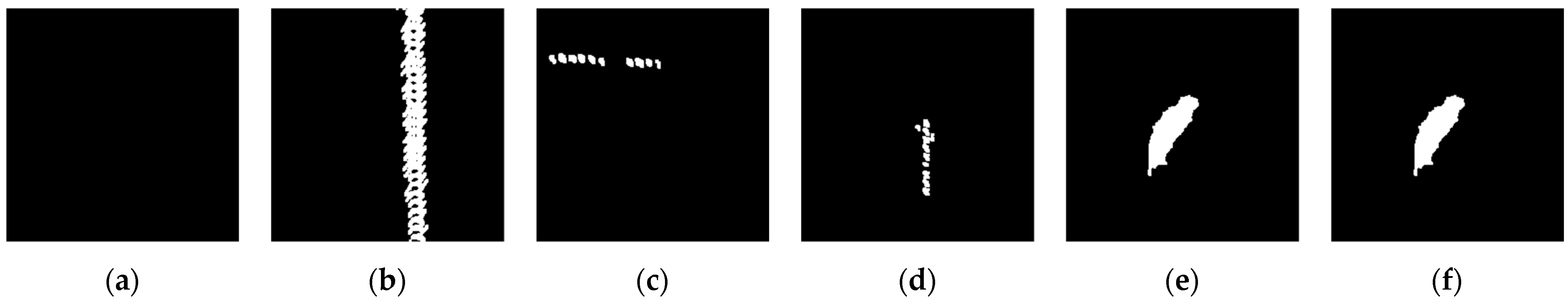
- By searching the outline in and combining , we finally locate the final position of the defect, as shown in Figure 10. In this paper, some small noise points are filtered out according to the contour area of the target.
3. Results and Discussion
- (1)
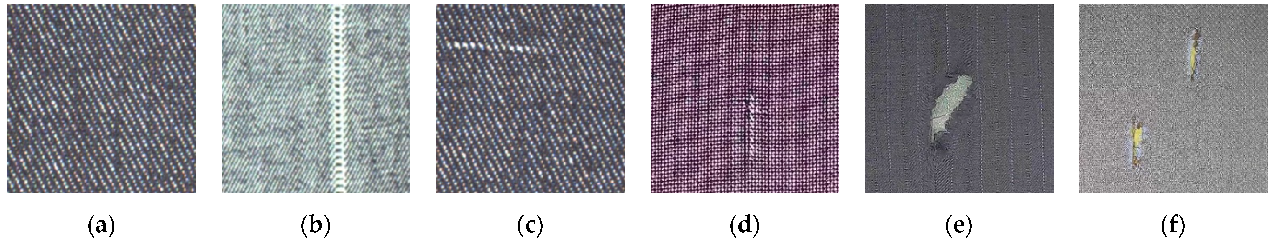
- From the direct visual comparison in Figure 11, it can be seen that the three comparison methods had good detection effects on the relatively obvious defect areas in the fabric image, but the detection effects on the complex-texture fabric image or the fabric image with no obvious defects were general, so its sensitivity was slightly lower than that of the method proposed in this paper.
- (2)
- The test set selected in this paper contained 100 fabric images with defects and 100 fabric images without defects. It can be seen from the parameter performance comparison in Table 2 that the three comparison methods easily misjudged the fabric images without defects as fabric images with defects, so the detection accuracy was reduced.
4. Conclusions
Author Contributions
Funding
Data Availability Statement
Conflicts of Interest
References
- Kumar, A. Computer-Vision-Based Fabric Defect Detection: A Survey. IEEE Trans. Ind. Electron. 2008, 55, 348–363. [Google Scholar] [CrossRef]
- Li, W.; Cheng, L. New progress of fabric defect detection based on computer vision and image processing. J. Text. Res. 2014, 35, 158–164. [Google Scholar]
- Cho, C.S.; Chung, B.M.; Park, M.J. Development of Real-Time Vision-Based Fabric Inspection System. IEEE Trans. Ind. Electron. 2005, 52, 1073–1079. [Google Scholar] [CrossRef]
- Jeyaraj, P.R.; Nadar, E.R.S. Effective textile quality processing and an accurate inspection system using the advanced deep learning technique. Text. Res. J. 2020, 90, 971–980. [Google Scholar] [CrossRef]
- Li, W.; Xue, W.; Cheng, L. Intelligent detection of defects of yarn-dyed fabrics by energy-based local binary patterns. Text. Res. J. 2012, 82, 1960–1972. [Google Scholar] [CrossRef]
- Wang, M.; Bai, R.; He, W.; Ji, F. Machine vision detection method of pattern fabric flaws. Opto-Electron. Eng. 2014, 41, 19–26. [Google Scholar]
- Hu, K.; Luo, S.; Hu, H. Improved algorithm of fabric defect detection using Canny operator. J. Text. Res. 2019, 40, 153–158. [Google Scholar]
- Sun, W.; Li, Q.; Shao, T.; Wu, H. Crack Detection Algorithm of Protective Wall for Piles Based on Machine Vision. Comput. Eng. Appl. 2019, 55, 260–265. [Google Scholar]
- Karimi, M.H.; Asemani, D. Surface defect detection in tiling industries using digital image processing methods: Analysis and evaluation. ISA Trans. 2014, 53, 834–844. [Google Scholar] [CrossRef]
- Hu, H.; Li, J.F.; Shen, J.M. Detection methods for surface micro defection on small magnetic tile based on machine vision. Mech. Electr. Eng. Mag. 2019, 36, 117–123. [Google Scholar]
- Zhang, E.H.; Chen, Y.J.; Gao, M.; Duan, J.; Jing, C. Automatic defect detection for web offset printing based on machine vision. Mach. Vis. 2020, 2020, 3598. [Google Scholar] [CrossRef] [Green Version]
- Li, C.; Li, C.; Wu, X.J.; Palade, V.; Fang, W. Effective method of weld defect detection and classification based on machine vision. Comput. Eng. Appl. 2018, 54, 264–270. [Google Scholar]
- Shojaedini, S.V.; Haghighi, R.K.; Kermani, A. A new method for defect detection in lumber images: Optimising the energy model by an irregular parametric genetic approach. Int. Wood Prod. J. 2017, 8, 26–31. [Google Scholar] [CrossRef]
- Cao, J.; Wang, N.; Zhang, J.; Wen, Z.; Li, B.; Liu, X. Detection of varied defects in diverse fabric images via modified RPCA with noise term and defect prior. Int. J. Cloth. Sci. Technol. 2016, 28, 516–529. [Google Scholar] [CrossRef]
- Zhu, S.; Hao, C. Fabric defect detection method based on texture periodicity analysis. Comput. Eng. Appl. 2012, 48, 163–166. [Google Scholar]
- Zhang, K.; Yan, Y.; Li, P.; Jing, J.; Liu, X.; Wang, Z. Fabric defect detection using salience metric for color dissimilarity and positional aggregation. IEEE Access 2018, 6, 49170–49181. [Google Scholar] [CrossRef]
- Qian, X.L.; Zhang, H.Q.; Zhang, H.L.; He, Z.D.; Yang, C.X. Solar cell surface defect detection based on visual saliency. Chin. J. Sci. Instrum. 2017, 38, 1570–1578. [Google Scholar]
- Essa, E.; Hossain, M.S.; Tolba, A.S.; Raafat, H.M.; Elmogy, S.; Muahmmad, G. Toward cognitive support for automated defect detection. Neural Comput. Appl. 2020, 32, 4325–4333. [Google Scholar] [CrossRef]
- Li, Y.; Luo, H.; Yu, M.; Jiang, G.; Cong, H. Fabric defect detection algorithm using RDPSO-based optimal Gabor filter. J. Text. Inst. Part 3. Technol. A New Century 2019, 110, 487–495. [Google Scholar] [CrossRef]
- Bo, Z.; Tang, C. A Method for Defect Detection of Yarn-Dyed Fabric Based on Frequency Domain Filtering and Similarity Measurement. Autex Res. J. 2019, 19, 257–262. [Google Scholar]
- Wang, L.; Zhong, Y.; Li, Z.; He, Y. Online detection algorithm of fabric defects based on deep learning. J. Comput. Appl. 2019, 39, 2125–2128. [Google Scholar]
- Wu, Z.; Zhuo, Y.; Li, J.; Feng, Y.; Han, B.; Liao, S. Fast detection algorithm of single color fabric defects based on convolution neural network. J. Comput. Aided Des. Comput. Graph. 2018, 30, 2262–2270. [Google Scholar]
- Achanta, R.; Hemami, S.; Estrada, F.; Susstrunk, S. Frequency-tuned Salient Region Detection. In Proceedings of the 2009 IEEE Conference on Computer Vision and Pattern Recognition (CVPR 2009), Miami, FL, USA, 20–25 June 2009; IEEE: New York, NY, USA, 2009; pp. 1597–1604. [Google Scholar]
- Achanta, R.; Estrada, F.; Wils, P.; Süsstrunk, S. Salient Region Detection and Segmentation. In Proceedings of the Computer Vision Systems, ICVS 2008, Santorini, Greece, 12–15 August 2008; pp. 66–75. [Google Scholar]
- Cheng, M.M.; Mitra, N.J.; Huang, X.; Torr, P.H.; Hu, S.M. Global Contrast Based Salient Region Detection. IEEE Trans. Pattern Anal. Mach. Intell. 2015, 37, 569–582. [Google Scholar] [CrossRef] [PubMed] [Green Version]
- Zhai, Y.; Shah, M.; Shah, P. Visual attention detection in video sequences using spatiotemporal cues. In Proceedings of the 14th Annual ACM International Conference on Multimedia, Santa Barbara, CA, USA, 23–27 October 2006; ACM Press: New York, NY, USA, 2006; pp. 815–824. [Google Scholar]


| 1. | The enhancement result obtained in Section 2.1 is represented with enhanceImg. Its size is M × N. M is the height, N is the width, and the size of the sliding window is 24, i.e., size = 24. The result of the preliminary location of defects is represented with locationImg. The result of binarization is represented with binaryImg. Mask results are represented with maskImg. |
| 2. 3. 4. 5. 6. 7. 8. 9. 10. 11. 12. 13. 14. 15. 16. 17. 18. 19. 20. 21. 22. 23. 24. 25. 26. 27. 28. 29. 30. 31. 32. 33. 34. 35. 36. 37. 38. 39. 40. 41. | For i = 0 : M For j = 0 : N subImg = enhanceImg(j, i, min(N − j , size), min(M − i, size)) Calculate the mean value of subImg, represented by m Calculate the variance of subImg, represented by sd Use a structure variable named subInfo to save the i, j, m, and sd, and then save it with a list named infoList infoList.push_back(subInfo) Save m with a list named meanList, and save sd with a list named sdList meanList.push_back(m) sdList.push_back(sd) j = j + size × 0.5 End i = i + size × 0.5 End Next, the outliers are obtained using the IQR method. Sort meanList and sdList from small to large length = meanList.size meanQ1 = meanList [0.25 × length] meanQ3 = meanList [0.75 × length] meanIQR = meanQ3 − meanQ1 meanUpper = meanQ1 − 2.5 × meanIQR meanDown = meanQ3 + 2.5 × meanIQR sdQ1 = sdList [0.25 × length] sdQ3 = sdList [0.75 × length] sdIQR = sdQ3 − sdQ1 sdUpper = sdQ1 − 2.5 × sdIQR sdDown = sdQ3 + 2.5 × sdIQR The defects are initially located according to the outliers of mean and variance For t = 0 : length mTmp = infoList[t].mean mSd = infoList[t].sd If mTmp > meanDown and mSd > sdDown Obtain the position of the current sub-image and save it to Rect r r.x = infoList[t].i, r.y = infoList[t].j r.width = min(N, width − r.x), r.height = min(M, height − r.y) Obtain the mask of the sub-image where the defect is located, maskImg(r) = 255 Copy this sub-image into locationImg, enhanceImg(r).copyto(locationImg(r)) Adaptive threshold binarization for this sub-image threshValue = min(40,infoList[t].mean × 10) Binarize the sub image with threshValue as the threshold and assign it to binaryImg (r) End |
| 42. | End |
| Detection Method | Acc | Precision | Recall | F1 | T (s) | ||||
|---|---|---|---|---|---|---|---|---|---|
| AC | 77 | 64 | 23 | 36 | 0.705 | 0.77 | 0.681 | 0.723 | 0.078 |
| HC | 65 | 68 | 35 | 32 | 0.665 | 0.65 | 0.670 | 0.659 | 0.061 |
| LC | 69 | 71 | 31 | 29 | 0.7 | 0.69 | 0.704 | 0.696 | 0.053 |
| Our method | 97 | 98 | 3 | 2 | 0.975 | 0.97 | 0.979 | 0.974 | 0.067 |
Disclaimer/Publisher’s Note: The statements, opinions and data contained in all publications are solely those of the individual author(s) and contributor(s) and not of MDPI and/or the editor(s). MDPI and/or the editor(s) disclaim responsibility for any injury to people or property resulting from any ideas, methods, instructions or products referred to in the content. |
© 2023 by the authors. Licensee MDPI, Basel, Switzerland. This article is an open access article distributed under the terms and conditions of the Creative Commons Attribution (CC BY) license (https://creativecommons.org/licenses/by/4.0/).
Share and Cite
Li, W.; Zhang, Z.; Wang, M.; Chen, H. Fabric Defect Detection Algorithm Based on Image Saliency Region and Similarity Location. Electronics 2023, 12, 1392. https://doi.org/10.3390/electronics12061392
Li W, Zhang Z, Wang M, Chen H. Fabric Defect Detection Algorithm Based on Image Saliency Region and Similarity Location. Electronics. 2023; 12(6):1392. https://doi.org/10.3390/electronics12061392
Chicago/Turabian StyleLi, Weiwei, Zijing Zhang, Mingyue Wang, and Hang Chen. 2023. "Fabric Defect Detection Algorithm Based on Image Saliency Region and Similarity Location" Electronics 12, no. 6: 1392. https://doi.org/10.3390/electronics12061392