Consensus-Based Distributed Optimal Dispatch of Integrated Energy Microgrid

Abstract

In recent years, the energy form of microgrids is constantly enriching, while the decentralization requirements of microgrids are constantly developing. Considering the economic benefits of an integrated energy microgrid (IEM), this paper focuses on the distributed optimal dispatch of IEM based on a consensus algorithm. The microgrid structure and multi-agent system are combined organically to get the decentralized architecture of IEM. This paper takes the incremental cost rate of each unit in IEM as a consensus variable. Based on the consensus theory, iterative optimization is carried out to achieve the optimal economic operation and power supply-demand balance of IEM. The distributed optimal dispatch is realized, and the convergence of the algorithm is proved. The experiment is carried out with LabVIEW and MATLAB and verifies the effectiveness of the algorithm. The results show that the distributed optimal dispatch algorithm can effectively reduce the power generation cost of the integrated energy system.

1. Introduction

With the intensification of the global energy crisis, and the current social demand for ecological civilization, the traditional centralized architecture of large power grids is beginning to change to the decentralized intelligent microgrid, and the form of energy in a microgrid is also developing towards diversification. The deep integration of power networks and the internet is causing significant changes in the consumption and use of electric energy [1]. The power industry is a basic and necessary industry of the national economy, which is related to all aspects of production and life. How to make the IEM system achieve the balance of power supply and demand, the construction of a well-functioning regulatory structure and economic optimal operation has become an important problem to be handled. These problems can be summed up as the economic dispatch problem (EDP) in the power grid system, and the EDP also exists in the IEM system.

Compared with centralized control, the multi-agent consensus technique has stronger autonomy, robustness and scalability. In addition, it can effectively reduce the consumption of communication resources and computing resources, and improve the operation efficiency of complex network systems. Based on the above advantages, multi-agent technology has been widely applied and researched in different disciplines, such as robot control [2], aerospace engineering [3], traffic control [4], power networks [5], etc.

With the improvement of the utilization rate of renewable energy, the proportion of distributed power generation in the power grid is increasing. It is of great significance and application prospect to use the multi-agent consensus technology to solve the coordinated control of distributed power in the power grid [6,7]. To accommodate current and future developments, the new generation of power systems will integrate communication control and distributed control. In [8] was proposed a method of economic optimal operation of isolated microgrids based on a distributed control algorithm, which has some in-depth research in economic dispatching. Comprehensive research on the grouping form and group-level coordination control of AC and DC microgrid clusters was done in the literature [9], which proposed an intelligent multi-level control approach based on a discrete consistency algorithm. The literature [10] designed a multi-intelligence-based microgrid operation decision support system structure. The mentioned distributed control of microgrids did not find a relevant discussion of IEMs concerning EDPs, and there is no overall experimental implementation of the consistency algorithm in combination with the host computer.

In terms of economic and stability optimization, the literature [11] uses a non-cooperative game method considering coupling constraints to solve the problem of electric vehicle charging scheduling. A new type of non-cooperative control mechanism in the literature [12], combining economic factors as well as physical constraints and grid stability, optimizes the operation of distribution networks equipped with traditional loads, distributed generation and active users. The above papers have verified different goals and effectively improved the dispatching and operation capabilities of new energy in the distribution network, but did not analyze the situation of IEM.

The consensus technique is used in this work to undertake a distributed optimum dispatch analysis for an IEM. The consensus-based distributed algorithm’s convergence is demonstrated, based on the principle of equal incremental cost rate of power system, and the consensus variable of IEM is determined. On the premise that the IEM takes into account the power balance and economic operation, the distributed optimal dispatching of the IEM is realized. Moreover, the human-machine interface (HMI) system with microgrids is constructed, which enriches the distributed architecture. Simulation in MATLAB/Simulink is used to verify the algorithm’s efficacy, while the distributed optimal dispatch is implemented based on LabVIEW platform in cooperation with MATLAB simulation.

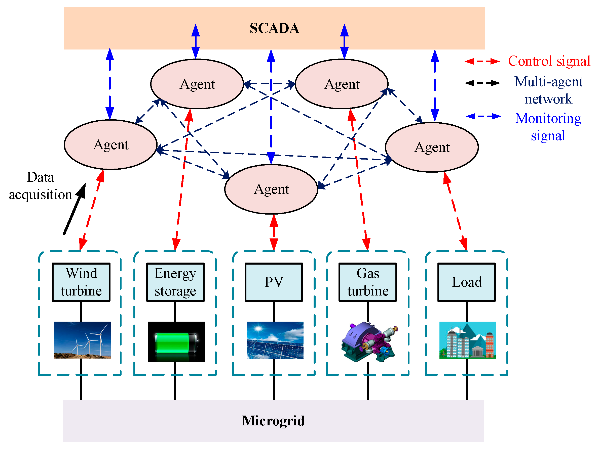
2. Decentralized Architecture for IEM

The deep integration of power grids and communication networks drives the evolution of regional energy systems toward large-scale physical energy systems. Microgrid is then gradually evolving towards an architecture that includes a physical layer including physical systems (e.g., power grids), a communication layer including communication systems (e.g., communication networks), and a data computation and optimization control layer (e.g., distributed algorithms) [13].

Microgrid implementation has considerably increased the amount of solar, wind, and other renewable energy sources, lowering power system costs, pollutant emissions, and environmental contamination. The flexibility of energy storage devices, microgrid system structure and power generation devices improve the utilization rate of electric energy. Appropriate control strategies can significantly improve the power quality and improve the economic indicators of the power grid. Each bus node of the microgrid topology has an associated agent that can communicate with its neighbors over a communication network. At the same time, between the physical and communication layers, there are intermediate units where the acquired data is processed and analyzed in order to perform distributed algorithms. This results in a multi-agent-based distributed architecture for an IEM as shown in Figure 1.

The definition of multi-agent varies among different research fields, and the connections between agents are important considerations in the system network. The communication network is the primary problem to apply a multi-agent algorithm in a microgrid. The system structure is the topology diagram G, the communication network structure diagram of the multi-agent microgrid system is defined as G = (V, E, A), and the set of nodes is denoted as V = {v₁, v₂, ⋯, v_i, ⋯, v_n}, where n represents the number of nodes and the number of micro-generators. The edge set between nodes is denoted by E, and the connectivity between adjacent nodes is expressed by A, that is, the n × n adjacency matrix [14]. Where communication is established between i-th and the j-th nodes, then create edge pair (v_i, v_j), which belongs to E, denotes as (v_i, v_j) ∈ E. N_i = {j|(i, j) ∈ E} denotes the collection of nodes that are linked to node i.

According to graph theory and matrix theory, the adjacency matrix can be solved to obtain the Laplace matrix. For the Laplace matrix elements L_ij between different adjacent nodes, assign corresponding weights W_ij(k), which can improve the convergence speed of the algorithm. Using the Metropolis (MA) algorithm, the weight matrix is:

$$W_{ij}=\left\{\begin{array}{ll}\frac{1}{\underset{i\in V}{\max }\left|L_{ii},L_{jj}\right|+1},\hfill & j\in N_i\\ 1-{\displaystyle \sum _{k\in N_i}\frac{1}{\underset{i\in V}{\max }\left|L_{ii},L_{kk}\right|+1},}\hfill & i=j,\\ 0,\hfill & \mathrm{others}\end{array}\right.$$

(1)

3. Decentralized Architecture for IEM

3.1. First-Order Consensus Theory

A consensus method is a way of describing the interaction behavior of a multi-agent system and thus, is called a consensus protocol [15,16]. The consensus algorithm is useful in a variety of situations, including synchronization phenomena, cluster motion, aggregation problems, and so on. The state of node i is denoted by xi. When all nodes in a network finally attain the same state, it is called consensus, i.e., x₁ = x₂ = ⋯ = x_n. The method of economic operation in microgrids mainly applies first-order discrete consensus algorithms, which are characterized by fast convergence and simple interaction logic. The dynamic equation of node i in a first-order discrete system is

$$x_i[k+1]={\displaystyle \sum _{j\in N_i}{c}_{ij}(x_j[k]-x_i[k])}+x_i[k]={\displaystyle \sum _{j=1}^n{c}_{ij}{x}_j[k]}$$

(2)

where k and c_ij represent the number of iterations and the connectivity of node i and node j, respectively.

3.2. Economic Optimization Control of IEM

The various parts of the IEM can be divided into three broad categories: generating components, energy storage entities, and load components. The penetration of distributed power sources in a microgrid is rising as distributed power sources continue to increase. As a result, modeling of diverse power sources is essential to assure the study’s universality. There are not only dispatchable power sources like photovoltaic power integrated energy storage, diesel generators, and micro gas turbines but also clean energy generation units including solar and wind power among the generators. A range of criteria, including generator efficiencies, prices of fuel, and the need for maintenance, must be considered when modeling the cost of each unit in a microgrid [17]. The modeling of the cost of micro-gas turbines, fuel cells, photovoltaic units with energy storage, flexible loads, etc., can be simplified to a unified model

$$C_i(P_i)={\gamma }_i+{\beta }_i{P}_i+{\alpha }_i{P}_i^2$$

(3)

where C_i is the generation cost of i-th micro source; P_i is the power; α_i, β_i, and γ_i are the cost coefficients.

The objective function of economic optimization is

$$\min C_{\mathrm{total}}={\displaystyle \sum _{i=0}^n{C}_{powe{r}_i}(P_{powe{r}_i})}+{\displaystyle \sum _{i=0}^n{C}_{loa{d}_i}(P_{loa{d}_i})}$$

(4)

where C_total is the total system cost, C_power,i is the cost of each generating unit, C_load,i is the cost of each load. Ultimately, the goal is to reduce the total cost of micro sources in a microgrid.

The constraints are made up of equality constraints and inequality constraints, where equality constraints are power supply and demand balance constraints, power flow constraints, and incremental cost model constraints of controllable micro sources.

$${\displaystyle \sum P_{loa{d}_i}}+{\displaystyle \sum P_{powe{r}_i}}=0$$

(5)

This means that the output power’s algebraic sum of all the generation units in the target system and the total load demand power is zero, regardless of losses.

When the grid operates stably, the system voltage and power must satisfy the power flow equation

$$\left\{\begin{array}{l}{P}_i=U_i{\displaystyle \sum _{j=1}^n{U}_j(G_{ij}\cos {\theta }_{ij}+B_{ij}\sin {\theta }_{ij})}\\ Q_i=U_i{\displaystyle \sum _{j=1}^n{U}_j(G_{ij}\sin {\theta }_{ij}-B_{ij}\cos {\theta }_{ij})}\end{array}\right.$$

(6)

where G_ij and B_ij are the conductance and susceptance between nodes ij respectively, θ_ij is the phase angle difference between nodes i and j. In this paper, the influence of network loss on the power flow calculation of the system is ignored, and only the power balance is considered. In the later research, the power flow calculation constraints will be added.

Each micro source then has an incremental cost rate:

$$d_i=\frac{\partial C_i}{\partial P_i}={\beta }_i+2{\alpha }_i{P}_i$$

(7)

Then the power of the i-th unit is formulated as

$$P_i=2{\alpha }_i^{-1}(d_i-{\beta }_i)$$

(8)

The inequality constraints are summarized at the end as

$$P_i(t)=\left\{\begin{array}{ll}{P}_{i,\min },\hfill & 2{\alpha }_i^{-1}(d_i-{\beta }_i)\le P_{i,\min }\\ 2{\alpha }_i^{-1}{d}_i-\beta ,\hfill & P_{i,\min }\le 2{\alpha }_i^{-1}(d_i-{\beta }_i)\le P_{i,\max }\\ P_{i,\max },\hfill & 2{\alpha }_i^{-1}(d_i-{\beta }_i)\ge P_{i,\max }\end{array}\right.$$

(9)

In the inequality constraint, since the network loss is not considered, node voltage constraints are added for the sake of system stability.

$$U_{i,\min }\le U_i\le U_{i,\max }$$

(10)

where U_i,min and U_i,max are the minimum and maximum values allowed by the node voltage deviation respectively.

The power of each generating unit and load does not exceed the corresponding upper and lower limits during system operation, i.e.,

$$P_{i,\min }\le P_i\le P_{i,\max }$$

(11)

3.3. Equal Incremental Cost Rate Principle of Microgrid

The Lagrange multiplier method is a widely used method for applying the equal incremental rate principle to microgrids, in which each generating unit operates at an equal incremental cost rate, resulting in the lowest total energy consumption and the most cost-effective operation [18]. Lagrange’s equation can be derived using the model, goal function, and restrictions mentioned in Section 3.2.

$$L={\displaystyle \sum _{i=1}^n{C}_i}+d({\displaystyle \sum _{i=1}^n{P}_i}-P_L)+{\displaystyle \sum _{i=1}^n{\underset{¯}{u}}_i}(P_i-P_{i,\min })+{\displaystyle \sum _{i=1}^n{\overline{u}}_i}(P_{i,\max }-P_i)$$

(12)

$$\frac{\partial L}{\partial P_i}=-d_i(P_i)+d-{\overline{u}}_i+{\underset{¯}{u}}_i=0$$

(13)

$$\frac{\partial L}{\partial d}=({\displaystyle \sum _{i=1}^n{P}_i}-P_L)=0$$

(14)

$$\frac{\partial L}{\partial {\overline{u}}_i}=P_{i,\max }-P_i\ge 0,\frac{\partial L}{\partial {\underset{¯}{u}}_i}=P_i-P_{i,\min }\ge 0$$

(15)

$${\overline{u}}_i(P_{i,\max }-P_i)=0,{\underset{¯}{u}}_i(P_i-P_{i,\min })=0$$

(16)

$${\overline{u}}_i\ge 0,{\underset{¯}{u}}_i\ge 0$$

(17)

To satisfy the conditions of Equations (13)–(17), Pi satisfies P_i,min ≤ P_i ≤ P_i,max, ${\overline{u}}_i={\underset{¯}{u}}_i=0$ can be obtained, substituting it into Equation (13) yields the optimal incremental cost rate d* = d_i (P_i). The optimal solution is

$$\left\{\begin{array}{ll}{d}_i=d^{*},\hfill & P_{i,\min }<p_i<P_{i,\max }\hfill \\ d_i\le d^{*},\hfill & p_i=P_{i,\max }\hfill \\ d_i\ge d^{*},\hfill & p_i=P_{i,\min }\hfill \end{array}\right.$$

(18)

As a result, when and only when the incremental cost rates of the controlled distributed micro sources are identical, the economic optimization model reaches an optimal result, resulting in the microgrid’s least generation cost. The reach of the lower or upper limit means the micro source arrives at the maximal or minimal cost rate limit. As a result, the solution of optimal economic dispatch can be derived using the law of equal incremental cost rate.

4. Consensus-Based Optimal Power Dispatch of IEM

4.1. Algorithm Description

A multi-agent consensus-based distributed control strategy for IEM is proposed in this paper. By setting the consensus variables and retrieving the information from the agent, the distributed control law makes the consensus variables of different power sources converge to the same value and finally achieve the control goal.

In order to solve the problem of economic dispatching and the balance of power supply-demand, it is necessary to calculate the optimal solution d* and the optimal output power in the whole system. In this paper, an appropriate incremental cost rate consensus algorithm is designed based on the consensus-based multi-agent system and the incremental rate principle of the power system. The algorithm incorporates the idea of distributed cooperative control without obtaining global information and relies on local interconnection and distributed cooperative control among agents. The ideal incremental cost rate and optimal output power may be reached by progressively bringing the consensus variables to the same value using the control law. The consensus-based distributed cooperative control strategy for hybrid IEM is described in detail as follows:

The initial values need to be calculated according to Equation (19) without participating in the iterations, and the calculation results are used as the known values for the second iteration.

$$\left\{\begin{array}{c}{\lambda }_i(0)=2{\alpha }_i{p}_i(0)+{\beta }_i\\ p_i(0)={\displaystyle \sum _{i=1}^n{p}_i(0)}=P_0\\ y_i(0)=0\end{array}\right.$$

(19)

Description of the iterative process of the algorithm:

$$\left\{\begin{array}{l}{\lambda }_i(k+1)={\epsilon }_i{y}_i(k)+{\displaystyle \sum _{j\in N_i}{\rho }_{ij}}{\lambda }_j(k)\\ p_i(k+1)=0.5{\alpha }_i^{-1}({\lambda }_i(k+1)-{\beta }_i)\\ y_i(k+1)={\displaystyle \sum _{j\in N_i}{\rho }_{ij}{y}_j(k)+p_i(k)-p_i(k+1)}\end{array}\right.$$

(20)

where λ_i is the incremental cost rate of the i-th agent, i.e., i-th micro source, ρ_ij is the state transfer matrix, ε_i is the non-negative feedback gain or control gain affecting the rate of convergence, the i-th micro source’s output power is denoted as p_i, and y_i denotes the local estimate of the imbalance of total demand-generation at each node. ε_i–y_i provides the shortage between generation and demand with ε_i as the feedback factor, and through continuous iterations, the optimal solution is eventually obtained.

The following is the algorithm’s specific implementation steps:

Step 1: To begin, create a cost estimate for each distributed micro source and load that makes up the hybrid IEM. For each micro source, the initial value of incremental cost rate (k = 0) is also preset.

Step 2: Determine the communication topology of the hybrid IEM, and at the same time construct the coefficient matrix of communication, to obtain the state transfer matrix containing weight factors, and build an objective function, as well as constraints based on the microgrid’s distributed cooperative control law.

Step 3: The output powers of the other linked micro sources are gathered by the micro source at the present time (t = k) and are then used to calculate the micro source’s local supply-demand mismatch of power. The consensus variable is then processed and introduced into the equation in order to get the reference power for the micro source at the following time step (t = k + 1).

Step 4: Finally, after several control cycles, all micro sources agree to increase the cost rate, thus reaching the economically optimal state.

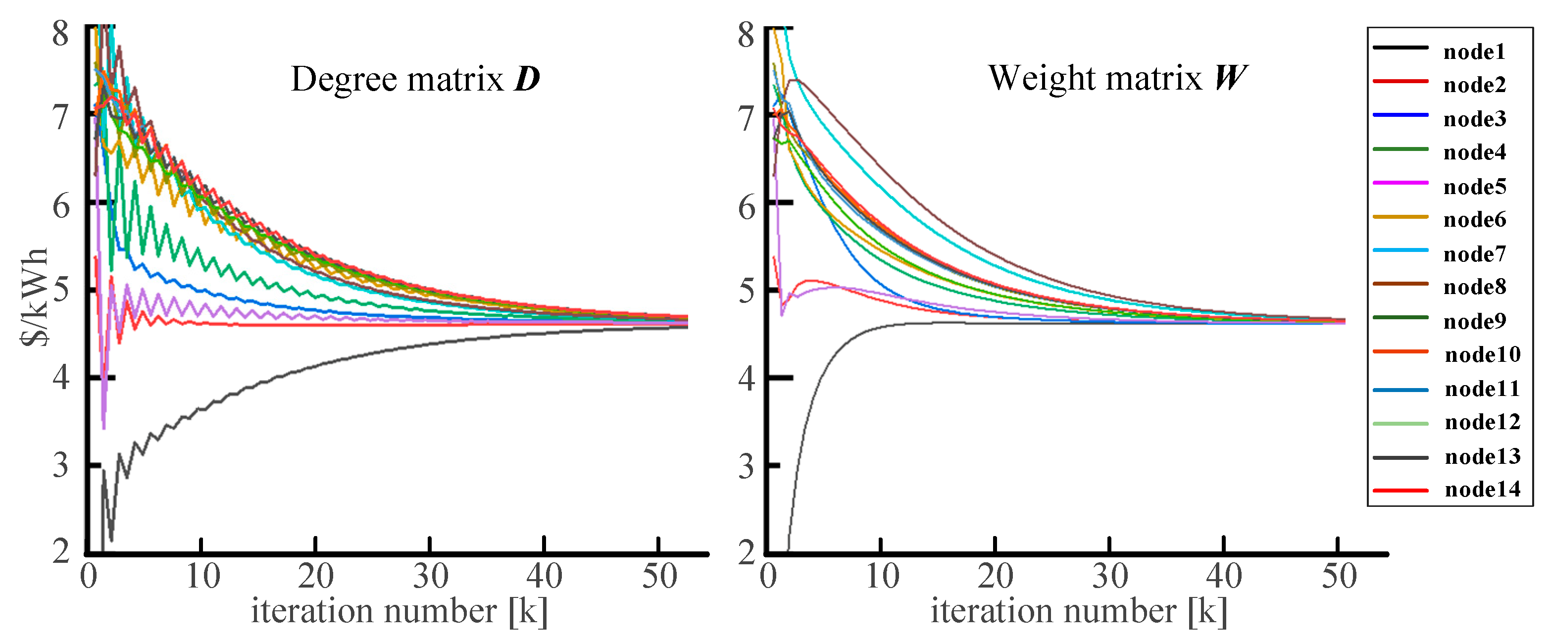
4.2. Convergence Proof

According to the literature [13], Equation (20) is rewritten into matrix form, and the n-dimensional column vectors of p_i, d_i, and y_i are denoted by P, D, and Z, respectively. Other variables have the forms as follows:

$$\begin{array}{l}\mathit{F}=\mathrm{diag}[0.5{\alpha }_1, 0.5{\alpha }_2, \dots , 0.5{\alpha }_n],\\ \mathit{B}=-{[0.5{\alpha }_1^{-1}{\beta }_1, 0.5{\alpha }_1^{-1}{\beta }_2, \dots , 0.5{\alpha }_1^{-1}{\beta }_n]}^{\mathrm{T}}\\ \mathit{E}=\mathrm{diag}[{\epsilon }_1, {\epsilon }_2, \dots , {\epsilon }_n]\end{array}$$

(21)

Thus, Equation (20) can be transformed into the following matrix forms:

$$\left\{\begin{array}{c}\mathit{D}(k+1)=\mathit{E}(k)\mathit{Z}(k)+\mathit{A}\mathit{D}(k)\\ \mathit{P}(k+1)=\mathit{B}+\mathit{F}\mathit{D}(k+1)\\ \mathit{Z}(k+1)=-[\mathit{P}(k+1)-\mathit{P}(k)]+\mathit{A}\mathit{Z}(k)\end{array}\right.$$

(22)

The matrix A is a double random matrix and can be acquired using Equation (22).

$$1^{\mathrm{T}}[\mathit{Z}(k+1)+\mathit{P}(k+1)]=1^{\mathrm{T}}[\mathit{Z}(k)+\mathit{P}(k)]=\cdots =1^{\mathrm{T}}[\mathit{Z}(0)+\mathit{P}(0)]$$

(23)

i.e., regardless of the value of k, ${\sum }_{i=0}^n[z_i(k)+p_i(k)]$ remains the same constant. Therefore, to balance the total power demand and generation, z_i (0) = 0 is chosen for all agents 1, 2, …, n. Let pi (k) be an arbitrary value and ${\sum }_{i=0}^n{p}_i(0)=P_0$. This gives the initial value of the algorithm

$$\left\{\begin{array}{c}{p}_i(0)={\displaystyle \sum _{i=1}^n{p}_i(0)}=P_0\\ d_i(0)={\beta }_i+2p_i(0){\alpha }_i\\ z_i(0)=0\end{array}\right.$$

(24)

This leads to the following results:

At the k-th iteration, the total power demand-supply mismatch is calculated to be ${\sum }_{i=0}^n{z}_i(k)=P_0-{\sum }_{i=0}^n{p}_i(k)$ i.e., z_i(k) represents mismatch values between the local power supply and demand. For all agents i = 1, 2, …, n, the system power supply-demand balance is reached if $z_i(k)\to \infty$ when $k\to \infty$. The optimal solution of the objective function without constraints is then acquired using the initial condition of Equation (24).

The optimal solution is reached when all of the incremental cost rates di converge to the identical state, according to Equation (22), i.e., the optimal value, and the mismatch between local power supply and demand is 0. Therefore, it is only required to prove that $d_i\to d^{\ast }$ and $z_i(k)\to 0$ when $k\to \infty$. To do this it is necessary to construct the matrix for the proof:

$$\mathit{M}=\left[\begin{array}{cc}\mathit{A}& \mathit{E}(k)\\ \mathit{F}(-\mathit{A}+\mathit{I})& -\mathit{F}\mathit{E}(k)+\mathit{A}\end{array}\right]$$

(25)

The negative terms $(-\mathit{A}+\mathit{I})$ are contained in the matrix M, hence the non-negative matrices theory is not to be employed in the analysis of the matrix M directly. Rewriting Equation (22) as

$$\left[\begin{array}{c}\mathit{Z}(k+1)\\ \mathit{D}(k+1)\end{array}\right]=\mathit{M}\left[\begin{array}{c}\mathit{Z}(k)\\ \mathit{D}(k)\end{array}\right]$$

(26)

Since the system matrix M is split into two matrices to make the proof easier:

$$\mathit{W}=\left[\begin{array}{cc}0& \mathit{E}(k)\\ 0& -\mathit{F}\mathit{E}(k)\end{array}\right],{\mathit{M}}_0=\left[\begin{array}{cc}\mathit{A}& 0\\ \mathit{F}(\mathit{I}-\mathit{A})& \mathit{A}\end{array}\right]$$

(27)

It can be seen that M is M₀, which is perturbed by vector $\mathit{q}=\left[{\epsilon }_1(k),{\epsilon }_2(k),\cdots ,{\epsilon }_n(k)\right]$. The theory of eigenvalue perturbations of matrices is applied to prove the convergence of the consistency algorithm [19]. Propositions on eigenvalue perturbations of matrices can be obtained from the literature [20].

When the two conditions, sufficiently small ${\epsilon }_1,{\epsilon }_2,\cdots ,{\epsilon }_n$ and strongly connected G, are satisfied, the optimal solution of the objective function can be solved using the initial value settings in Equation (26), i.e., the asymptotical convergence of $d_i$ and $p_i$ to optimal values $d^{*}$ and $p^{*}$ can be obtained, respectively.

M₀ is a lower triangular matrix, than the spectral radius $\rho ({\mathit{M}}_0)=\rho (\mathit{A})$. Additionally, $\rho (\mathit{A})=\mathbf{1}$ based on the fact that A is a doubly random matrix. The matrix A has a simple eigenvalue of 1 and the other eigenvalues with modulo less than 1 since A is irreducible and at the same time G is strongly connected. Therefore, the matrix M₀ has also a semi-simple eigenvalue of 1 and the remaining with modulo less than 1 [21]. It can be concluded that A has a right n-dimensional vector 1 since the conditions of the Perron–Forbenius theorem are satisfied by A. Thus, A has a left eigenvector $1^{\mathrm{T}}$, which is correlated with 1.

Make

$${\mathit{u}}_1=\left[\begin{array}{c}0\\ n^{-1}1\end{array}\right], {\mathit{u}}_2=\left[\begin{array}{c}1\\ -\alpha n^{-1}1\end{array}\right], {\mathit{v}}_1^{\mathrm{T}}=\left[\begin{array}{cc}{1}^{\mathrm{T}}\mathit{F}& 1^{\mathrm{T}}\end{array}\right],{\mathit{v}}_2^{\mathrm{T}}=\left[\begin{array}{cc}{n}^{-1}{1}^{\mathrm{T}}& 0^{\mathrm{T}}\end{array}\right]$$

(28)

where $\alpha ={\displaystyle {\sum }_{i=1}^{n}0.5{\alpha }_i^{-1}}$ is the column vector with n zero elements, u₁ are u₂ right eigenvector of M₀ and v₁, v₂ are left eigenvectors of M₀, respectively. Then there is ${\left[\begin{array}{cc}{\mathit{v}}_1^{\mathrm{T}}& {\mathit{v}}_2^{\mathrm{T}}\end{array}\right]}^T\left[\begin{array}{cc}{\mathit{u}}_1& {\mathit{u}}_2\end{array}\right]=\mathit{I}$.

The following is calculated according to the matrix eigenvalue perturbation theory

$$\left[\begin{array}{cc}{\displaystyle \sum _{i=1}^n({\mathit{v}}_1^{\mathrm{T}}\frac{\partial \mathit{W}}{\partial {\epsilon }_i}{\mathit{u}}_1)}& {\displaystyle \sum _{i=1}^n({\mathit{v}}_1^{\mathrm{T}}\frac{\partial \mathit{W}}{\partial {\epsilon }_i}{\mathit{u}}_2)}\\ {\displaystyle \sum _{i=1}^n({\mathit{v}}_2^{\mathrm{T}}\frac{\partial \mathit{W}}{\partial {\epsilon }_i}{\mathit{u}}_1)}& {\displaystyle \sum _{i=1}^n({\mathit{v}}_2^{\mathrm{T}}\frac{\partial \mathit{W}}{\partial {\epsilon }_i}{\mathit{u}}_2)}\end{array}\right]$$

(29)

The matrix M has the following Jordan canonical form

$$\mathit{M}=\mathit{Q}\mathit{J}{\mathit{Q}}^{-1}=\left[\begin{array}{ccc}{\mathit{q}}_1& \cdots & {\mathit{q}}_{2n}\end{array}\right]\mathrm{diag}(1,{\mathit{J}}_1){\left[\begin{array}{ccc}{\mathit{r}}_1^{\mathrm{T}}& \cdots & {\mathit{r}}_{2n}^{\mathrm{T}}\end{array}\right]}^T$$

(30)

The left and right eigenvectors of the matrix M have the following form ${\mathit{q}}_1={\alpha }^{-1}{\left[\begin{array}{cc}{1}^{\mathrm{T}}& 0^{\mathrm{T}}\end{array}\right]}^{\mathrm{T}}$, ${\mathit{r}}_1^{\mathrm{T}}={\alpha }^{-1}\left[\begin{array}{cc}{1}^{\mathrm{T}}\mathit{F}& 1^{\mathrm{T}}\end{array}\right]$, which corresponds to eigenvalue 1. When $k\to \infty$ there is

$${\mathit{M}}^k=\mathit{Q}{\mathit{J}}^k{\mathit{Q}}^{-1}=\mathit{Q}\mathrm{diag}(1,{\mathit{J}}_1^k){\mathit{Q}}^{-1}$$

(31)

which leads to

$${\mathit{q}}_1{\mathit{r}}_1^{\mathrm{T}}={\alpha }^{-1}\left[\begin{array}{cccccc}0.5{\alpha }_1^{-1}& \cdots & 0.5{\alpha }_n^{-1}& 1& \cdots & 1\\ ⋮& & ⋮& ⋮& & ⋮\\ 0.5{\alpha }_1^{-1}& \cdots & 0.5{\alpha }_n^{-1}& 1& \cdots & 1\\ 0& \cdots & 0& 0& \cdots & 0\\ ⋮& & ⋮& ⋮& & ⋮\\ 0& \cdots & 0& 0& \cdots & 0\end{array}\right]$$

(32)

From the initial values $d_i(0)=2{\alpha }_i{p}_i(0)+{\beta }_i$ and $z_i(0)=0$, we have ${\left[\begin{array}{cc}{\mathit{D}}^{\mathrm{T}}(k)& {\mathit{Z}}^{\mathrm{T}}(k)\end{array}\right]}^{\mathrm{T}}={\mathit{M}}^k{\left[\begin{array}{cc}{\mathit{D}}^{\mathrm{T}}(0)& {\mathit{Z}}^{\mathrm{T}}(0)\end{array}\right]}^{\mathrm{T}}$$\to d^{\ast }{\left[\begin{array}{cc}{1}^{\mathrm{T}}& 0^{\mathrm{T}}\end{array}\right]}^{\mathrm{T}}$, $d^{*}$ represents the optimal incremental rate of cost. The power supply-demand is thus balanced when the incremental cost rates of micro sources reach a consensus at $k\to \infty$.

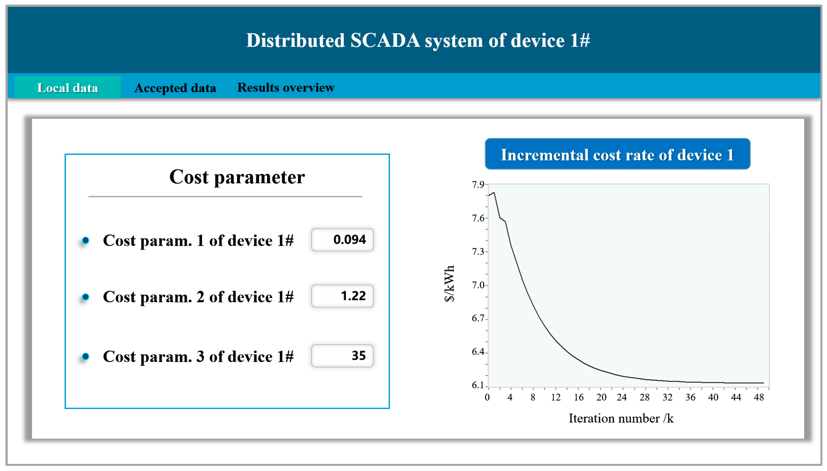
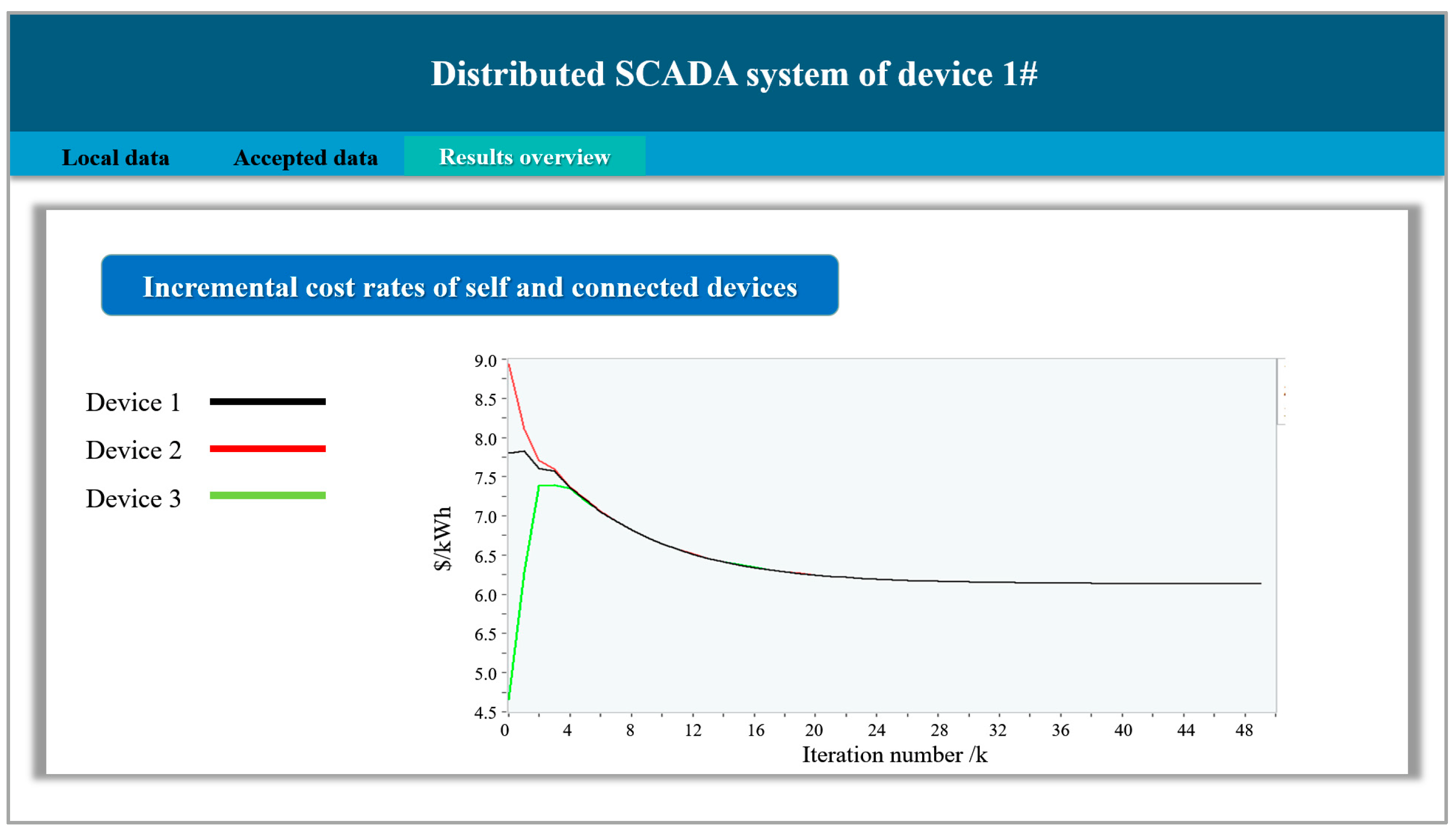
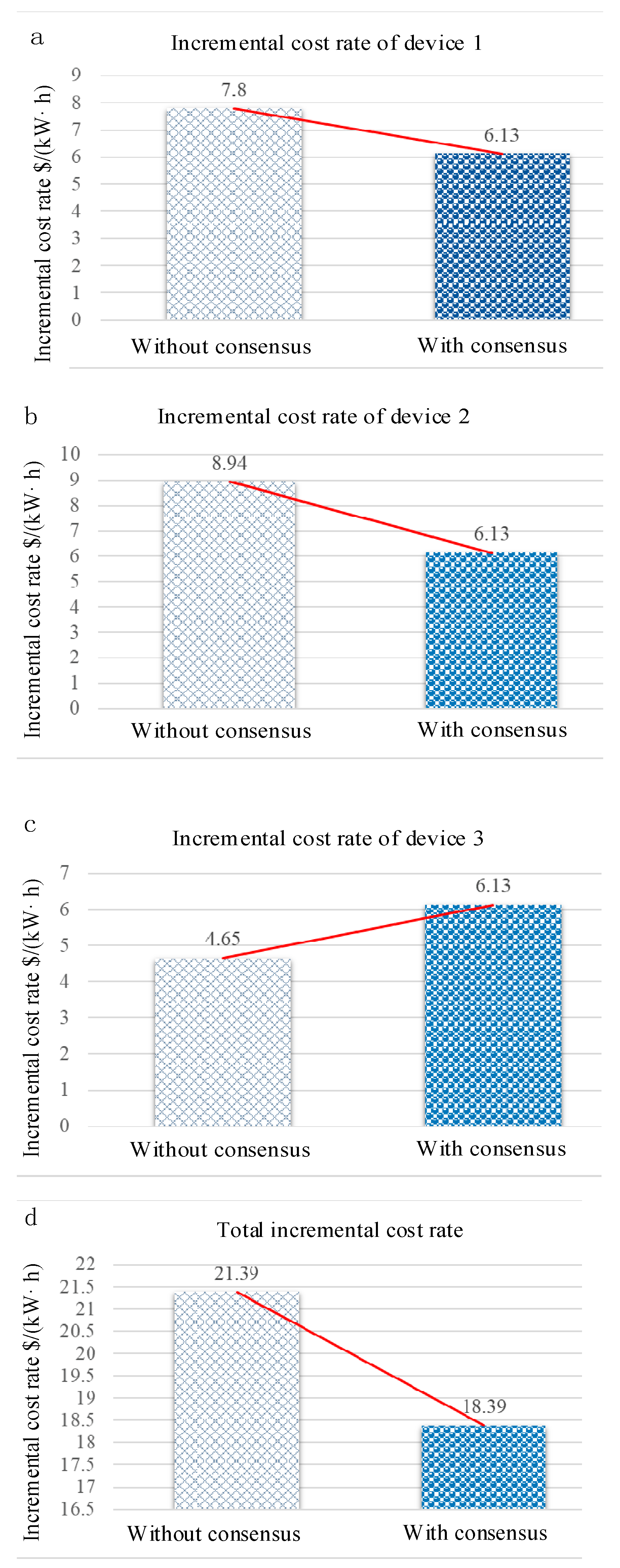
5. Experiment and Simulation Analysis

In this paper, the efficacy of consensus-based distributed optimal power dispatch is verified by simulation experiments with MATLAB software, and further distributed experiments are conducted based on the LabVIEW platform with MATLAB software. The simulation is carried out for an IEEE 14-Bus IEM system. Figure 2 and

Table 1. Cost Parameters of IEEE 14-Bus [22].

Node	Pi	αi	βi
1	0	0.020	0.14
2	0	0.062	4.20
3	0	0.075	3.25
4	0	0.072	8.25
5	0	0.066	7.20
6	0	0.070	4.05
7	0	0.350	0
8	0	0.075	7.80
9	0	0.060	8.05
10	0	0.078	8.45
11	0	0.080	8.75
12	0	0.085	9.00
13	0	0.069	7.05
14	0	0.077	8.15

present the topology and the specific system parameters of the system, respectively.

First, the degree matrix and adjacency matrix of the 14-bus IEM system need to be calculated to obtain the Laplacian matrix L of the system, and the weight matrix W of the system is further calculated according to formula (1) as the state transition matrix of the system. The initial basic parameters of the 14-bus system are shown in Table 1, where α_i and β_i are the cost parameters of each node.

Figure 3 depicts the result of the simulation. From Figure 3a. It can be seen that the 14 nodes achieve the same incremental cost rate of 5.31$/kW·h and satisfy the equal consumption incremental rate principle. Thus, the economically optimal operation is achieved. From Figure 3b,c, it can be seen that the nodes reach the power balance of supply and demand. The algorithm is verified as effective.

According to the comparison shown in Figure 4, the simulation results obtained by selecting the D matrix are more volatile, and the simulation results obtained by the W matrix are relatively smooth.

The distributed experiment based on the LabVIEW platform and MATLAB software aims to realize the consensus-based distributed optimal dispatch of IEM with a communication network. The overall schematic diagram of the experimental platform is shown in Figure 5a. The establishment of the communication network guarantees the information interaction of the agents and combines the high computational power of MATLAB and the user-friendly HMI of LabVIEW, leveraging their respective strengths to achieve distributed optimal dispatch.

The experiment is carried out with three computers equipped with MATLAB and LabVIEW software. Each computer is regarded as a node and a network cable is used to connect the three computers to a communication switch to ensure data interaction between the computers. The distributed optimization dispatch algorithm is based on MATLAB, and the algorithm program in MATLAB is called LabVIEW.

The specific experiment steps as shown in Figure 4b are as follows:

Step 1: Write the main program of the distributed collaborative method on the three computers in MATLAB, which is detailed in Section 4.1.

Step 2: All three devices create a project based on LabVIEW software and create a visual identity (VI).

Step 3: Create databases in the created project based on the distributed collaborative algorithm, add all variables to the databases and set them as shared variables.

Step 4: Integrate the server (1) and client (2) of the transmission control protocol (TCP) multiple-connection program in the VI created and configure the internet protocol (IP) address and port number.

Step 5: Utilize the MATLAB script node to call the program described in Step 1 and configure the inputs and outputs used by the algorithm.

Step 6: Design the HMI on each of the three devices to implement the distributed supervisory control and data acquisition (SCADA) system.

Step 7: Connect the three devices to the communication switch and run the program until a consensus is reached.

The experimental results for one of the devices are shown in Figure 6 and Figure 7.

Based on the cost parameters of each device and the initial power, the incremental cost rate without iteration is calculated and compared with the consensus convergence results of distributed optimal dispatch algorithm, the results are shown in Figure 8a–d.

The incremental cost rates for devices 1, 2 and 3 without the consensus-based dispatch are $7.80/kW·h, $8.94/kW·h, and $4.65/kW·h, respectively. And from the experimental results, it is seen that the three units yield a convergence consensus result of 6.13$/kW·h with the integration of the distributed optimal dispatch algorithm. The incremental cost rate for devices 1 and 2 is reduced by 21.41%, and 31.43%, respectively. The total incremental cost rate reduction for all three devices, as shown in Figure 8d, is 14.03%. It can be concluded that the proposed distributed consensus-based algorithm effectively reduces the power generation cost of the whole IEM system.

6. Conclusions

This work provides a distributed optimum dispatch method for IEMs based on consensus theory. Each node in the system updates its local parameters via information interaction to achieve a consistent incremental cost rate and achieve the most economical operation of the IEM system. The algorithm’s convergence is demonstrated, and the approach’s efficacy is confirmed by simulation experiments conducted on distributed software systems. The results demonstrate that the distributed optimum dispatch method used in this article lowers system generation costs considerably. In order to facilitate the calculation of constraints, this paper ignores the influence of line loss on power flow. Factors such as line losses, charging and discharging costs of energy storage units, such as batteries and algorithm optimization at the power electronics level need to be considered in the further research of the IEM and consensus algorithm. Taking the economy and stability as comprehensive factors, it is necessary to consider the problem of multi-objective optimization.

References

1. Hao, R.; Ai, Q.; Zhu, Y. Cooperative optimal control of energy internet based on multi-agent consistency. Autom. Electr. Power Syst. 2017, 41, 10–17, 57. [Google Scholar]
2. Do, H.; Hong, S.; Kim, J. Robust Loop Closure Method for Multi-Robot Map Fusion by Integration of Consistency and Data Similarity. IEEE Robot. Autom. Lett. 2020, 5, 5701–5708. [Google Scholar] [CrossRef]
3. Han, J.; Shi, H.; Tong, J.; Zhang, Q.; Li, J. Time consistency technique of multi-aircrafts simulation system for cooperative mission. In Proceedings of the 2019 14th IEEE Conference on Industrial Electronics and Applications (ICIEA), Xi’an, China, 19–21 June 2019; pp. 1006–1010. [Google Scholar]
4. Qian, L.; Xu, X.; Zeng, Y.; Huang, J. Deep, Consistent Behavioral Decision Making with Planning Features for Autonomous Vehicles. Electronics 2019, 8, 1492. [Google Scholar] [CrossRef] [Green Version]
5. Mojumdar, M.R.R.; Cano, J.M.; Orcajo, G.A. Estimation of Impedance Ratio Parameters for Consistent Modeling of Tap-Changing Transformers. IEEE Trans. Power Syst. 2021, 36, 3282–3292. [Google Scholar] [CrossRef]
6. Yao, M.; Molzahn, D.K.; Mathieu, J.L. An optimal power-flow approach to improve power system voltage stability using demand response. IEEE Trans. Control. Netw. Syst. 2019, 6, 1015–1025. [Google Scholar] [CrossRef]
7. Mignoni, N.; Scarabaggio, P.; Carli, R.; Dotoli, M. Control frameworks for transactive energy storage services in energy communities. Control. Eng. Pract. 2023, 130. [Google Scholar] [CrossRef]
8. Meiqin, M.; Rui, X. Economic dispatch method for islanding microgrids based on distributed control. J. Electr. Eng. 2018, 13, 8–13. [Google Scholar]
9. Yang, G.; Qian, A.; Jing, W. Consensus cooperative control of AC/DC hybrid microgrids based on multi-agent system. High Volt. Eng. 2018, 44, 2372–2377. [Google Scholar]
10. Yingfeng, X.; Haining, W. Structure of decision support system based on multi-agent for micro-grid operation. J. Electr. Eng. 2016, 11, 30–36, 49. [Google Scholar]
11. Zhang, L.; Li, Y. A game-theoretic approach to optimal scheduling of parking-lot electric vehicle charging. IEEE Trans. Veh. Technol. 2016, 65, 4068–4078. [Google Scholar] [CrossRef]
12. Scarabaggio, P.; Carli, R.; Dotoli, M. Noncooperative equilibrium-seeking in distributed energy systems under AC power flow nonlinear constraints. IEEE Trans. Control. Netw. Syst. 2022, 9, 1731–1742. [Google Scholar] [CrossRef]
13. Wang, R.; Li, Q.; Zhang, B.; Wang, L. Distributed consensus-based algorithm for economic dispatch in a microgrid. IEEE Trans. Smart Grid 2019, 10, 3630–3640. [Google Scholar] [CrossRef]
14. Pu, T.; Liu, W.; Chen, N.; Wang, X.; Dong, L. Distributed optimal dispatching of active distribution network based on consensus algorithm. Proc. CSEE 2017, 37, 1579–1590. [Google Scholar]
15. Olfati-Saber, R.; Murray, R.M. Consensus problems in networks of agents with switching topology and time-delays. IEEE Trans. Autom. Control. 2004, 49, 1520–1533. [Google Scholar] [CrossRef] [Green Version]
16. Olfati-Saber, R.; Fax, J.A.; Murray, R.M. Consensus and cooperation in networked multi-agent systems. Proc. IEEE 2007, 95, 215–233. [Google Scholar] [CrossRef] [Green Version]
17. Rahbari-Asr, N.; Ojha, U.; Zhang, Z.; Chow, M. Incremental welfare consensus algorithm for cooperative distributed generation/demand response in smart grid. IEEE Trans. Smart Grid 2014, 5, 2836–2845. [Google Scholar] [CrossRef]
18. Chen, G.; Ren, J.; Feng, E. Distributed Finite-Time Economic Dispatch of a Network of Energy Resources. IEEE Trans. Smart Grid 2016, 8, 822–832. [Google Scholar] [CrossRef]
19. Cai, K.; Ishii, H. Average consensus on arbitrary strongly connected digraphs with time-varying topologies. IEEE Trans. Autom. Control. 2014, 59, 1066–1071. [Google Scholar] [CrossRef] [Green Version]
20. Chen, W.; Li, X.; Jiao, L. Quantized consensus of second-order continuous-time multi-agent systems with a directed topology via sampled data. Automatica 2013, 49, 2236–2242. [Google Scholar] [CrossRef]
21. Dai, Z.; Xie, H. Condition number of semi-simple eigenvalue of quadratic eigenvalue problem. Numer. Math. A J. Chin. Univ. 2017, 39, 153–167. [Google Scholar]
22. Li, S. Research on Distributed Cooperative Control of AC-DC Hybrid Microgrid; NCUT: Beijing, China, 2018. [Google Scholar]
Figure 1. Decentralized architecture for IEM.
Electronics 12 01468 g001
Figure 2. IEEE 14-Bus IEM system.
Electronics 12 01468 g002
Figure 3. Simulation results of the 14-Bus system (a) incremental cost rates (b) output powers of nodes (c) shortage of power.
Electronics 12 01468 g003
Figure 4. Comparison of D matrix and W matrix simulation results.
Electronics 12 01468 g004
Figure 5. Set up the experimental platform (a) Schematic diagram of the experiment platform (b) Implementation steps of the experiment.
Electronics 12 01468 g005
Figure 6. Local Data of device 1.
Electronics 12 01468 g006
Figure 7. Device 1 shows the consensus of the incremental cost rates.
Electronics 12 01468 g007
Figure 8. Incremental cost rate without and with consensus algorithm of (a) device 1, (b) device 2, (c) device 3, (d) Total incremental cost rate of the 3 devices.
Electronics 12 01468 g008