AoI-Bounded Scheduling for Industrial Wireless Sensor Networks

Abstract

Age of information (AoI) is an emerging network metric that measures information freshness from an application layer perspective. It can evaluate the timeliness of information in industrial wireless sensor networks (IWSNs). Previous research has primarily focused on minimizing the long-term average AoI of the entire system. However, in practical industrial applications, optimizing the average AoI does not guarantee that the peak AoI of each data packet is within a bounded interval. If the AoI of certain packets exceeds the predetermined threshold, it can have a significant impact on the stability of the industrial control system. Therefore, this paper studies the scheduling problem subject to a hard AoI performance requirement in IWSNs. First, we propose a low-complexity AoI-bounded scheduling algorithm for IWSNs that guarantees that the AoI of each packet is within a bounded interval. Then, we analyze the schedulability conditions of the algorithm and propose a method to decrease the peak AoI of nodes with higher AoI requirements. Finally, we present a numerical example that illustrates the proposed algorithm step by step. The results demonstrate the effectiveness of our algorithm, which can guarantee bounded AoI intervals (BAIs) for all nodes.

1. Introduction

Industrial wireless sensor networks (IWSNs) have emerged as a key technology enabling the deployment of Industry 4.0 for their flexibility, lack of wiring, low cost, and easy deployment characteristics [1]. IWSNs are capable of delivering time-sensitive periodic data flows generated by field devices to the gateway timely and reliably [2]. They have been widely deployed in industrial process automation applications, such as digital twin and remote state estimation [3]. These applications typically use data-driven models, and the data inputted into the model should be fresh enough to accurately characterize physical objects [4]. An emerging application layer performance metric, age of information (AoI), has recently been proposed to measure the freshness of data [5]. AoI is defined as the amount of time that has elapsed since the most recent update was generated at the source and successfully received at the destination [6]. Compared with traditional performance indicators (such as delay), AoI not only considers the time spent by data packets in wireless link transmission but also considers the transmission interval specified by the network scheduler. A small AoI implies that there exist fresh data available at the destination. AoI comprehensively characterizes the freshness of data packets, which can be applied to the performance evaluation of IWSNs.

Industrial applications require a high degree of data freshness, as many industrial processes are dynamic and rapidly changing [7]. Timely and accurate information is critical in making decisions that can impact the efficiency, safety, and overall performance of industrial operations [8]. For instance, in industrial process control systems, real-time data from sensors are essential to adjust process parameters, prevent equipment failures, and optimize production. In predictive maintenance, fresh data from sensors can be used to monitor the condition of machinery and predict potential failures before they occur, allowing for proactive maintenance and reducing downtime. If the age of information (AoI) for a certain amount of data falls below its corresponding threshold, it can result in significant damage to industrial production.

Due to the real-time nature of industrial applications, the IWSN standards (e.g., ISA100.11a and WirelessHART [9]) adopt time/frequency division multiple access (TDMA/FDMA) as the medium access method to achieve collision-free transmissions [2]. A network scheduler in the gateway assigns time slots and channels to transmit a flow to the destination, with multiple time slots in a superframe repeating cyclically [10]. Over the past decade, researchers have proposed various IWSN scheduling algorithms [11,12,13,14,15,16], focusing on minimizing transmission latency, energy consumption optimization, avoiding conflicts, etc. Some studies have proposed using AoI as a metric to measure the freshness of data in WSN. For instance, the authors in [4] analyze the long-term average AoI in WSN, and they formulate the AoI minimization problem subject to energy and time constraints. In [17,18], the authors consider minimizing the average AoI in energy constrained scenarios, especially the energy-harvesting WSN. Meanwhile, the authors of [19] derive the worst case average AoI and average peak AoI of data packets in WSN with the MAC layer based on a carrier sense multiple access with collision avoidance (CSMA/CA) method. However, optimizing AoI from the application layer perspective with hard performance requirements in IWSNs has rarely been considered.

Numerous studies have investigated AoI optimization problems in wireless networks [20], mainly focused on optimizing the performance of the whole system, taking into account different types of queue models, packet generation/arrival processes, queue capacities, wireless channel models, etc. For example, the authors in [5] discussed the minimum AoI for various single-service queue models under the first-come-first-served queue discipline. In [21], the authors derived an expression for the long-term average AoI of multi-service queue models. The authors of [22] investigated the problem of minimizing the AoI in a network subjected to various interference constraints and experiencing time-varying channels. The authors of [23] examined the optimal sampling and updating processes for IoT devices in a real-time monitoring system to minimize the long-term average AoI. In summary, most studies on AoI optimization scheduling based on queue theory aim to target a weighted-sum long-term average AoI. There are also some works focused on reducing the violation probability, where the peak AoI exceeds a given age constraint [24,25,26]. However, the reduction of violation probability still cannot meet the deterministic requirements of industrial applications. The authors of [27] proposed a scheduling algorithm with the constraint that each source in the system has a maximum AoI threshold. They assumed that the time is divided into slots and each source node collects a new sample at the beginning of each slot. Nonetheless, it is still challenging for sensor nodes in IWSNs to sample data at each time slot due to computing capability and energy constraints.

In industrial applications, the timely delivery of sampled data from the source to the destination is critical, where there is a hard performance requirement for the AoI metric per data packet. It warrants attention that optimizing the average AoI does not guarantee a bounded peak AoI for each data packet; in industrial control systems, if one or a certain packet’s AoI exceeds the predetermined threshold, it can seriously affect the stability of the industrial control system. In view of this, we propose an AoI-bounded scheduling algorithm for IWSNs that ensures that the AoI of all data packets sent by each node in the network is within a bounded interval, thus ensuring that the peak AoI of all nodes is bounded, which is crucial for ensuring the stability of the system. The main contributions of this work can be summarized as follows.

• We propose a low-complexity AoI scheduling algorithm for IWSNs that ensures that each packet’s AoI is within a bounded interval, instead of optimizing the network’s long-term average AoI. To the best of our knowledge, this is the first work in IWSNs that guarantees that the AoI of each data packet is within a bounded interval, which meets the high real-time demands of industrial applications.
• We analyze the schedulability conditions of the network and propose a method for reducing the peak AoI of nodes with higher AoI requirements by allocating more time slots to those nodes.
• We provide a numerical example to demonstrate the algorithm step by step, and the results show the effectiveness of our algorithm.

The rest of this paper is organized as follows. In Section 2, the system model and problem statement are presented by means of a comparison of the AoI evolution process for data packets at different transmission intervals, and Section 3 presents our AoI-bounded scheduling algorithm and analyzes the bounded AoI intervals (BAIs) of nodes. The performance of the proposed algorithm is evaluated and discussed in Section 4. The conclusions are presented in Section 5.

2. System Model and Problem Statement

We consider a data collection scenario in a time-slotted IWSN consisting of one sink node and $N$ source nodes with a single hop. Each source node $N_i$ collects data periodically according to its own sampling period $T_i$ and sends packets to the sink through the wireless channel. We assume that the wireless channel is error-free, allowing us to ignore the underlying communication channel and simplify the scheduling policy design. The sampling period of nodes in an IWSN usually varies significantly due to differences in sensor type or data update rates required by the industrial application. We assume that each sensor node adopts a single-packet queue model due to the low-power and low-cost characteristics of IWSNs. In this model, the older packet is dropped from the queue when a new packet is generated. Therefore, to ensure the freshness and continuity of sampled data, the data packet in the queue must be transmitted to the sink node before the next new periodic data packet generation. The main notations used throughout this paper are summarized in

Table 1. List of key notations.

Notation	Description
$i$	Index for node
$t$	Time slot number
$X_i\left(t\right)$	Indicator function that is equal to 1 when the node $i$ transmits the packet in time slot $t$, and $X_i\left(t\right)=0$ otherwise
$G_i\left(t\right)$	Data generation time
$A_i\left(t\right)$	The AoI of source node $i$ at time slot $t$
$T_i$	Sampling period of node $i$
${\Delta }_i^p$	Peak AoI of the of node $i$
$I_i$	Transmission interval time of node $i$
$U_{min}$	Minimum transmission units
${\alpha }_i$	Transmission interval coefficient of node $i$
${{\rm P}}_t$	The duration of a superframe

.

The IEEE 802.15.4 is commonly adopted in IWSNs as the physical and MAC layer fundamental techniques [2]. Assuming that the system is synchronized, time is divided into equal-length time slots. Let $X_i\left(t\right)\in \left\{0,1\right\}$ be the indicator function that is equal to 1 when the node $i$ transmits the packet in time slot $t$, and $X_i\left(t\right)=0$ otherwise. It should be noted that interference may arise when multiple nodes transmit packets during the same time slot, and therefore, at most, one packet can be transmitted in the one slot, since we have

$${{\displaystyle \sum }}_{i=1}^N{X}_i\left(t\right)\le 1.$$

(1)

Similar to [27,28], we assume that a node will wait until its send time slot to transmit a data packet that it has generated, instead of sending it immediately. Each source node can send data to the sink node and receive an acknowledgment message within a single time slot. The scheduler cyclically schedules each source node through a superframe with a duration of $P_t$. The packet sent by a source node comprises the data and the data generation time, denoted by $G_i\left(t\right)$. The AoI of source node $i$ at time $t$ is represented by $A_i\left(t\right)$. When the sink successfully receives a new packet, $A_i\left(t\right)$ is updated to the difference between the current time slot $t$ and $G_i\left(t\right)$. In other cases, $A_i\left(t\right)$ increases linearly. The update process of $A_i\left(t\right)$ can be expressed as follows:

$$A_i\left(t\right)=\{\begin{array}{l}t-G_i\left(t\right)+1 \mathrm{if}\mathrm{node}i\mathrm{update}\\ A_i\left(t-1\right)+1 \mathrm{others}\end{array}.$$

(2)

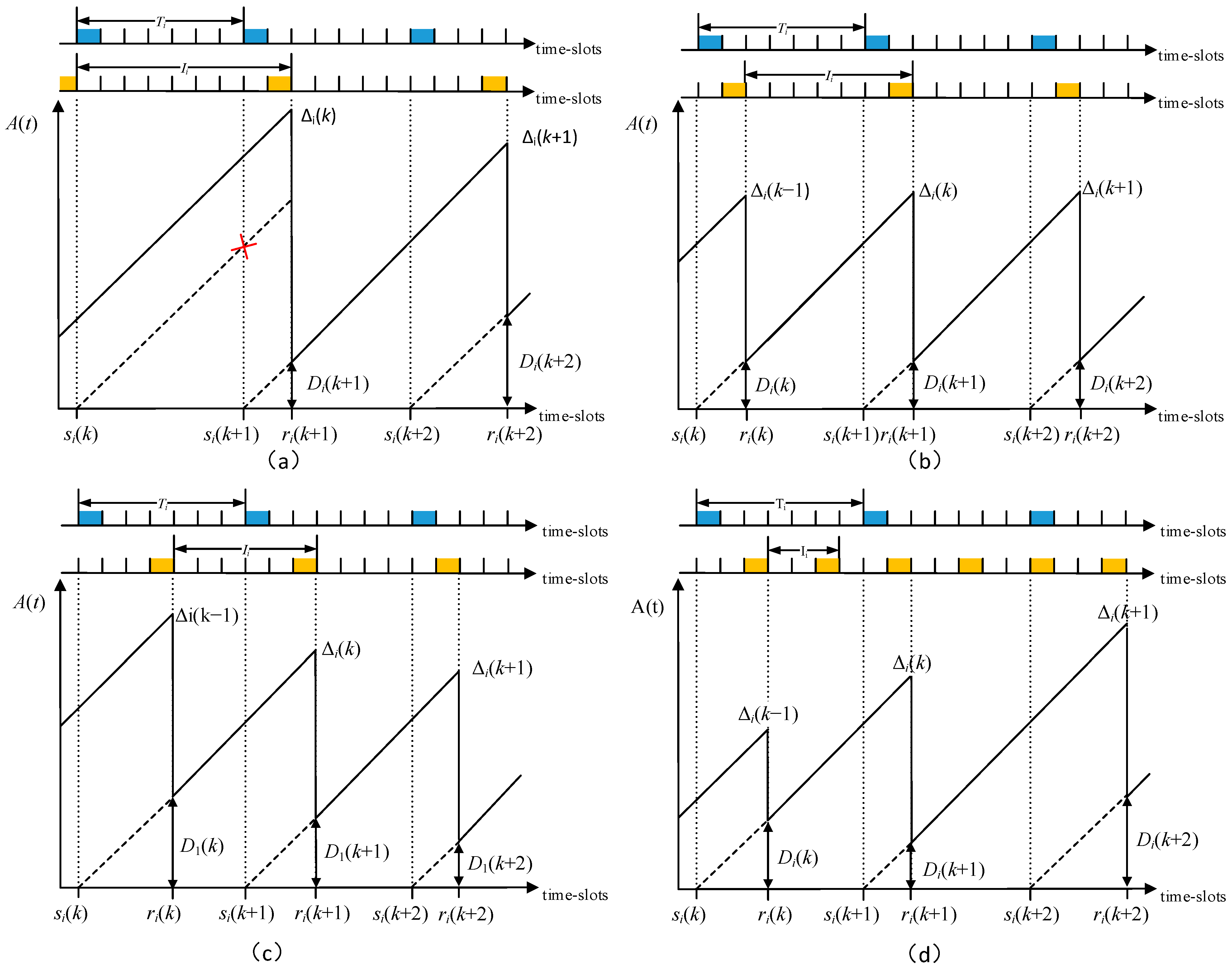
Figure 1 presents a comparison of the AoI evolution process of packets under different transmission intervals with the same sampling period ($T_i=7$) of a node. The upper part of each subgraph illustrates the data sampling events and data packet transmission events in time slots, while the lower part depicts the AoI evolution process according to different generation and delivery sequences of data packets. The sampling event of the source node occurs at time slot $s_i\left(k\right),s_i\left(k+1\right),\cdots$, and the sink node receives the corresponding data packet at time slot $r_i\left(k\right),r_i\left(k+1\right),\cdots$. We define the peak AoI of the k-th packet of node $i$ as ${\Delta }_i^p\left(k\right),\forall k>0$. The time between packet generation and sink reception is referred to as the system time $D_i\left(k\right)$, which is equal to $r\left(k\right)-s\left(k\right)$. We refer to the transmission interval time as $I_i$, which equals $r\left(k+1\right)-r\left(k\right)$.

The source node in our system employs a single packet queue model, which means that any data packet not sent from the queue will be dropped upon the generation of a new data packet. As shown in Figure 1a, where $I_i=9$ is greater than $T_i$, the packet k was not sent to the sink node before packet k + 1 was generated, resulting in the packet k being dropped. The red cross in Figure 1a indicates the moment that the data packet was dropped. To avoid packet drops, it is crucial that $I_i$ must be less than or equal to $T_i$. Ideally, the transmission interval for each source node would be equal to its own sampling period, with the time interval between the packet generation time slot and the transmission time slot kept as short as possible. As shown in Figure 1b, in this scenario, the AoI of the node changes periodically with the peak AoI being equal to $D_i\left(k\right)+I_i$ time slots (i.e., one time slot plus seven time slots equals eight time slots). However, it is impractical to ensure that the transmission interval of each node is equal to its own sampling period in a scheduling since the sampling period of nodes in an IWSN usually varies significantly. In Figure 1c,d, it can be clearly observed that a smaller transmission interval does not necessarily improve AoI performance but can instead cause a waste of time slots.

Based on (2), it can be inferred that in the absence of new message arrivals, the AoI of a node shows a linear growth with a slope of 1. From Figure 1, it can be observed that the peak AoI ${\mathsf{\Delta }}_i^p\left(k\right)$ of the k-th packet of node $i$ is calculated as the sum of the system time of the current data packet and its transmission interval. As such, we can conclude that

$${\mathsf{\Delta }}_i^p\left(k\right)=D_i\left(k\right)+\left[\frac{T_i}{I_i}\right]\times I_i,$$

(3)

where $\left[·\right]$ is the floor function. After the scheduler completes the network scheduling, the network executes the scheduling table repeatedly until the network parameters change. During the execution of the scheduling table, the value of $I_i$ remains fixed. Here, the peak AoI of a node is determined by system time $D_i$. Figure 1 also depicts that ${\Delta }_i\left(k\right)$ is equivalent to the transmission period added to the system time of the subsequent data packet and is expressed as

$${\mathsf{\Delta }}_i^p\left(k\right)=D_i\left(k+1\right)+T_i.$$

(4)

By substituting (4) into (3), we have the update process of $D_i\left(k\right)$ as

$$D_i\left(k+1\right)=\{\begin{array}{l}{D}_i\left(k\right)+\left[\frac{T_i}{I_i}\right]\times I_i-T_i,{\mathrm{if}\mathsf{\Delta }}_i^p\left(k\right)>T_i\\ D_i\left(k\right)+\left[\frac{T_i}{I_i}\right]\times I_i-T_i,\mathrm{others}\end{array}.$$

(5)

The value of $D_i\left(k\right)$ changes periodically, which leads to the value of ${\Delta }_i\left(k\right)$, as stated in (4), being within a specific period. However, it is an intractable problem to determine the transmission interval $I_i$ of nodes. If the value of $I_i$ is less than or equal to $T_i$, it guarantees that there will be at least one time slot between two consecutive sampling slots. On the other hand, if $I_i$ is greater than $T_i$, there will be no send time slot between two consecutive sampling time slots of a node. This consequently results in the node being unable to send the current data before the next sampling data are generated, ultimately leading to discarding the existing data. According to (4) and (5), when $I_i=T_i$, the node’s peak AoI will be a specific value, and the duration of the superframe can be the least common multiple of $T_i$. Therefore, it is challenging to determine the length of the superframe due to the considerable variance in the nodes’ sampling period. However, the value of $\frac{1}{I_i}$ indicates the proportion of the slot occupied by node $i$ in a superframe. Thus, ${\displaystyle \sum }_{i=1}^N\frac{1}{I_i}\le 1$ is necessary for the network to satisfy the scheduling feasibility. Therefore, we must choose an appropriate $I_i$ for the node according to $T_i$.

3. AoI-Bounded Scheduling Algorithm

This section first presents the AoI-bounded scheduling algorithm for IWSNs. Then, we analyze the BAI of nodes with different sampling periods under this algorithm. Finally, we propose a method for improving the BAI in the proposed algorithm for nodes with higher AoI requirements.

3.1. Scheduling Algorithm

The algorithm primarily divides the superframe into multiple minimum transmission units $\left(U_{min}\right)$ with the same length. Each node’s $I_i$ is an integer multiple of $U_{min}$ and less than its $T_i$, guaranteeing that each node sends the current data before the next sampled data are generated and that the network’s schedulability is satisfied.

As $U_{min}$ is the algorithm’s basic scheduling unit in a superframe, it is necessary to ensure that the $U_{min}$ is less than or equal to the minimum sampling period in all nodes to prevent data packets from being dropped. However, since $I_i$ is an integer multiple of $U_{min}$, a larger $U_{min}$ can cause a superframe to have more available time slots. We take the minimum $T_i$ among all nodes as the $U_{min}$, which can be obtained as

$$U_{min}=min\left\{T_i,\forall i\in N\right\}.$$

(6)

$U_{min}$ is taken as the least common factor of the transmission interval $I_i$ for each node. $I_i$ represents the length of the interval between two adjacent transmission time slots of node $i$ within one superframe. The $I_i$ of node $i$ can be obtained as

$$I_i\left(k\right)={\alpha }_i\times U_{min},$$

(7)

and

$${\alpha }_i=2^{\left[{\log }_2\left(\frac{T_i}{U_{min}}\right)\right]}.$$

(8)

${\alpha }_i$ is the transmission interval coefficient (TIC) of node $i$, defined as a power of two, i.e., $2^n$. $\left[·\right]$ is a floor function. According to (8), $I_i<T_i$.

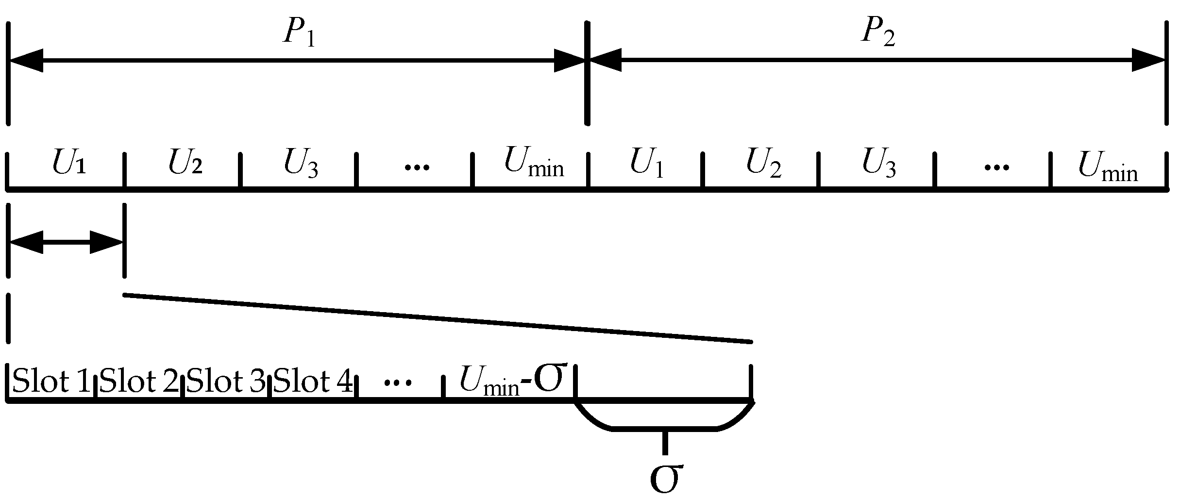
In addition to considering periodic data transmission, aperiodic data cannot be ignored. We reserve $\sigma$ time slots for aperiodic data packets in each $U_{min}$; this means that there are $U_{min}-\sigma$ time slots that can be allocated to periodic data flows in each $U_{min}$. The general structure of the superframe defined by the proposed scheduling algorithm is shown in Figure 2. When considering network scheduling feasibility, it is crucial to ensure that the time slots allocated for periodic nodes as well as the reserved time slots of aperiodic nodes should not exceed the length of $U_{min}$, as constrained by condition (9):

$${{\displaystyle \sum }}_{i=1}^N\frac{1}{{\alpha }_i}+\sigma \le U_{min}.$$

(9)

Under the condition of guaranteeing network scheduling feasibility, by (9), each node’s transmission intervals $I_i$ are multiples of each other. The duration of a superframe $P_t$ is the least common multiple of all nodes $I_i$. Thus, $P_t$ can be obtained as

$$P_t=max\left({\alpha }_i\right)\times U_{min},i\in \left[1,N\right].$$

(10)

Finally, dedicated time slots are assigned to each node. In this step, priority is given to nodes with a smaller $T_i$ to determine their initial scheduling time slot (IST). We allocate the first unused time slot $t$ from 1 to $U_{k_i}$ as the IST of node $N_i$. After determining the IST, the corresponding time slots of $N_i$ in the remaining time slots of the superframe are determined accordingly, i.e., $IST+I_i\times m$, $m=\left[1,\cdots ,\frac{{\alpha }_{max}}{{\alpha }_i}-1\right]$. Take node $i$ with its ${\alpha }_i=2$ and the maximum $\alpha$ of the network (i.e., $k_{max}=8$) as an example. If there exists a time slot $\mathrm{t}\in \left[1,2\times U_{min}\right]$ with ${\displaystyle \sum }_{i=1}^N{X}_i\left(\mathrm{t}\right)=0$, we allocate the time slot $t$ as the IST of node $i$, and the corresponding time slots in the remaining superframe can be determined as $t+m\times I_i,\mathrm{m}\in \left\{1,2,3\right\}$. The key steps of the proposed algorithm are given in Algorithm 1. The time is mainly consumed in Step 5 of Algorithm 1, in which we need to find the first unused time slot for each node as its IST. Therefore, the time complexity of Algorithm 1 is $O\left(n^2\right)$, where $n$ denotes the number of nodes in the networks.

Algorithm 1: AoI-bounded Scheduling
	Input: N, $T_i$
	Output: $U_{min}$, IST, $P_t$, $I_i$
1	Determine the length of $U_{min}$ based on (6)	// step 1
2	for $i$ = 1,2,$\cdots$,$N$ do	// step 2
3	Determine the transmission interval $I_i$ of node $N_i$ based on (7) and (8).
4	end
5	// Validate the scheduability of the network.	// step 3
6	if ${\displaystyle \sum }_{i=1}^N\frac{1}{{\alpha }_i}+\sigma \le U_{min}$ then
7	Network is schedulable, go to Step 4;
8	else
9	Indicates the network configuration is overloaded;
10	Return;
11	end
12	Determine the duration of superframe $P_t$ based on (10);	// step 4
13	for $i$ = 1,2,$\cdots$,$N$ do	// step 5
14	//Assign dedicated time slots to each node
15	Allocate the first unused time slot t from 1 to $U_{k_i}$ as the IST of node $N_i$;
16	end
17	Return

3.2. BAI Analysis

In this section, we analyze the upper and lower bounds of the node AoI under the proposed scheduling algorithm, which in turn shows that the node AoI is in a bounded interval. The BAI of node $i$ can be determined by the interval between the minimum peak AoI and the maximum peak AoI.

The worst-case scenario for scheduling occurs when the send time slot of a node overlaps with a sample time slot, causing the latest sampled value to be delayed until the next send time slot. This delay results in the node’s AoI reaching its maximum value. In the worst-case scenario, the latest sampled data is generated after an elapsed time of $T_i$ from the last packet generation. Therefore, the AoI of the node at this time is $T_i$. The next sending time of the node requires $I_i$ time slots, and given that it takes one time slot to complete the transmission of the message, the maximum peak AoI ${\mathsf{\Delta }}_i{}^{max}$ of the node can be expressed as follows:

$${\mathsf{\Delta }}_i{}^{max}=I_i+T_i+1$$

(11)

Figure 1c depicts the optimal scenario of the scheduling algorithm, wherein a node immediately transmits sampled data in the following time slot. This allows the node to promptly send its data to the sink node and results in the minimum AoI for the node. In this case, with an additional time slot accounting for data packet transmission, the minimum peak AoI ${\mathsf{\Delta }}_i{}^{min}$ is given by

$${\mathsf{\Delta }}_i{}^{min}=1+T_i.$$

(12)

The analysis above indicates that the maximum and minimum peak AoI of a node is associated with its sampling period and transmission interval. Once the network scheduling concludes, both the sampling and transmission intervals remain constant, resulting in the AoI of the node being confined within a bounded interval. The BAI of node $i$ is between the maximum peak AoI ${\mathsf{\Delta }}_i{}^{max}$ and the minimum peak AoI ${\mathsf{\Delta }}_i{}^{min}$, i.e., $A_i\left(t\right)\in \left[I_i+T_i+1,T_i+1\right]$.

3.3. Peak AoI Decrease Method

From (7) and (11), we can determine that the maximum peak AoI is positively correlated with ${\alpha }_i$ and $U_{min}$. Improving the peak AoI by reducing $U_{min}$ will reduce the available time slots and affect network scheduling feasibility. The most effective way to improve BAI is to reduce the peak AoI of node $i$ by reducing ${\alpha }_i$. After reducing ${\alpha }_i$ to $\widetilde{{\alpha }_i}$, the the node’s $I_i\left(k\right)$ reduces accordingly, adding the node’s $\frac{P_t}{U_{min}}\times \left(\frac{1}{\widetilde{{\alpha }_i}}-\frac{1}{{\alpha }_i}\right)$ transmission slot to the superframe. The improved ${\mathsf{\Delta }}_i{}^{max}$ can be obtained as

$${\mathsf{\Delta }}_i{}^{max}=\frac{I_i\times \widetilde{{\alpha }_i}}{{\alpha }_i}+T_i+1.$$

(13)

Due to the addition of time slots for nodes, reducing the value of ${\alpha }_i$ must still satisfy constraint (8), ensuring network scheduling feasibility. Other than that, reducing the maximum peak AoI can also reduce the average AoI. According to [29], the average AoI ${\mathsf{\Delta }}_i$ of source node $i$ can be obtained as

$$\begin{gathered} {\mathsf{\Delta }}_i=\frac{E\left[D_i{T}_i\right]+E\left[T_i{}^2\right]/2}{E\left[T_i\right]} \\ {\mathsf{\Delta }}_i=E\left[D_i\right]+\frac{T_i}{2} \end{gathered}$$

(14)

Considering that the data packet transmission needs one time slot, the exception of $D_i$ can be obtained as

$$E\left[D_i\right]=\frac{1+I_i}{2}+1.$$

(15)

Therefore, a decrease in ${\alpha }_i$ will decrease BAI and the average AoI ${\mathsf{\Delta }}_i$, accordingly.

4. Evaluation and Numerical Results

In this section, we evaluate the performance of the proposed algorithm by providing an example and presenting the results of simulations. We consider a network of 10 sensor nodes that periodically sample data and send them to the sink node, i.e., $N=10$. The sampling period $T_i$ of each sensor node is uniformly distributed at random integers between 2 and 50 time slots, i.e., $T_i\in \left[2,50\right]$, as shown in

Table 2. Parameters setting of the example network.

Node ID	${\mathit{T}}_{\mathit{i}}$	${\mathit{\alpha }}_{\mathit{i}}$	${\mathit{I}}_{\mathit{i}}\left(\mathit{k}\right)$	IST
1	28	4	28	9
2	10	1	7	2
3	15	2	14	4
4	38	4	28	12
5	17	2	14	5
6	20	2	14	6
7	7	1	7	1
8	29	4	28	10
9	35	4	28	11
10	14	2	14	3

. The duration of a time slot is defined as 10 ms. We reserve one time slot for aperiodic data in each $U_{min}$. Following the five key steps of the proposed algorithm in Section 4, we present a detailed example below to illustrate the values obtained from each step of the proposed algorithm.

In step 1, the length of the minimum transmission unit $U_{min}$ is determined according to (6), which involves taking the minimum $T_i$ among all nodes. Since the sampling period of node #7 is the smallest among all nodes, the $U_{min}$ is set to seven time slots.

In step 2, the minimum scheduling unit and the sampling period of all nodes are given. Each node’s $I_i$ and ${\alpha }_i$ are calculated using Equations (7) and (8), respectively. The results are presented in Table 2.

In step 3, the primary task is to examine the schedulability of the network. According to (2), the sum of the reciprocal of coefficients for all nodes, adding the number of reserved time slots for aperiodic data packets, is calculated as ${\displaystyle \sum }_{i=1}^N\frac{1}{{\alpha }_i}+\sigma =6$, less than the $U_{min}$. This indicates that the proposed AoI scheduling algorithm can find a solution that schedules all the nodes under the current network parameters setting.

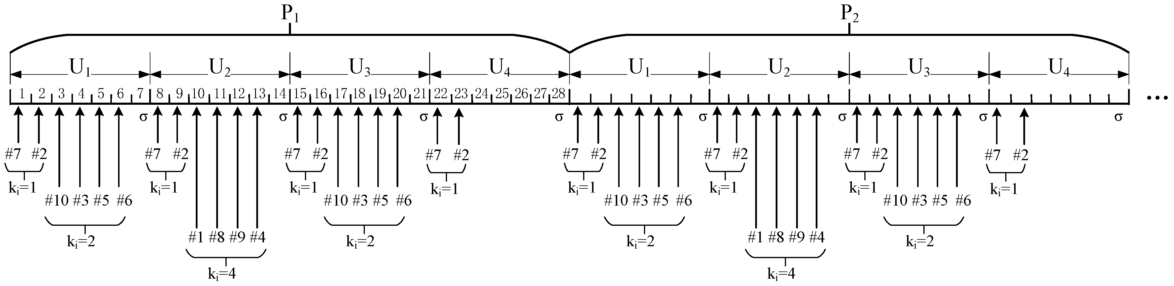
In step 4, the duration of the superframe is determined based on (10), i.e., $P_t=28$. The network will repeat the whole schedule table every 28 time slots.

In step 5, the dedicated time slots for each source node are allocated. Following the allocation process, the lower sampling period nodes are prioritized. For any node, its IST is determined, and then the remaining time slots are allocated according to $I_i\left(k\right)$. Table 2 shows each node’s IST, and Figure 3 shows each source node’s send time slot in a superframe. We take node #2 as an example, where ${\alpha }_2=1$; we need to decide the IST of node #2 in ${\mathrm{U}}_1$. Since time slot 1 is occupied by node #7, the IST of node 2 is set to time slot 2. According to (7), the transmission interval of node 2 is seven time slots. Thus, the time slots of node 2 in the superframe are 2, 9, 16, and 23.

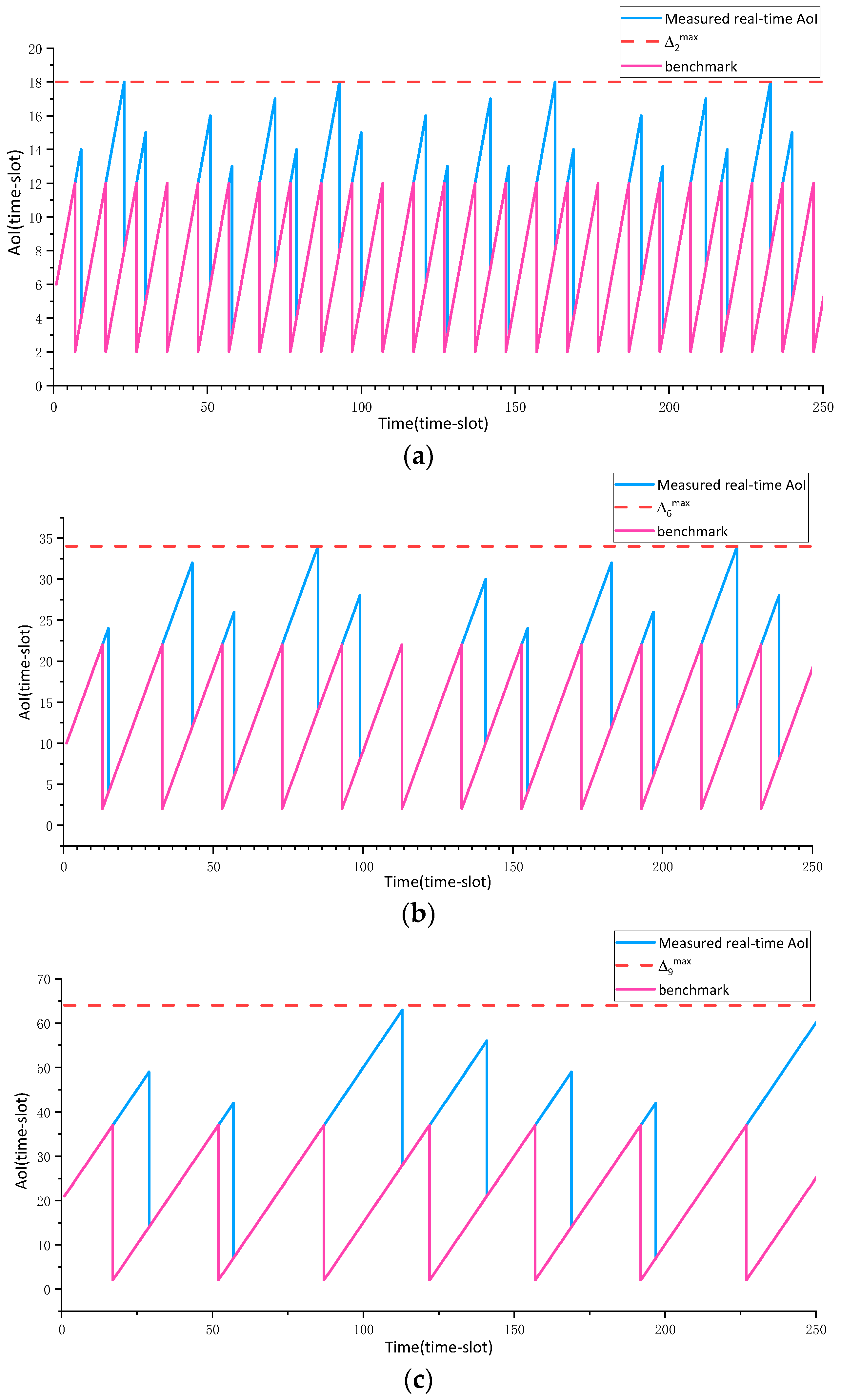
According to the parameters in Table 2, we evaluated the AoI performance of nodes in a discrete-event simulator that we built in a Python environment. To demonstrate the effectiveness of the proposed algorithm in ensuring AoI within a bounded interval, we selected three representative nodes and examined the changes in their AoI. These nodes include node #2 with ${\alpha }_2=1$, node #6 with ${\alpha }_6=2$, and node #9 with ${\alpha }_9=4$. We adopted the optimal greedy scheduling algorithm as a benchmark for comparison, in which each node transmits the data to the sink node in the next time slot after completing the sampling process, thereby obtaining the lower bound value of the peak AoI. It is crucial to note that it is impractical to apply the greedy scheduling strategy on every node in the network, given the large number of nodes and the possibility of significant variations in the sampling period of each node.

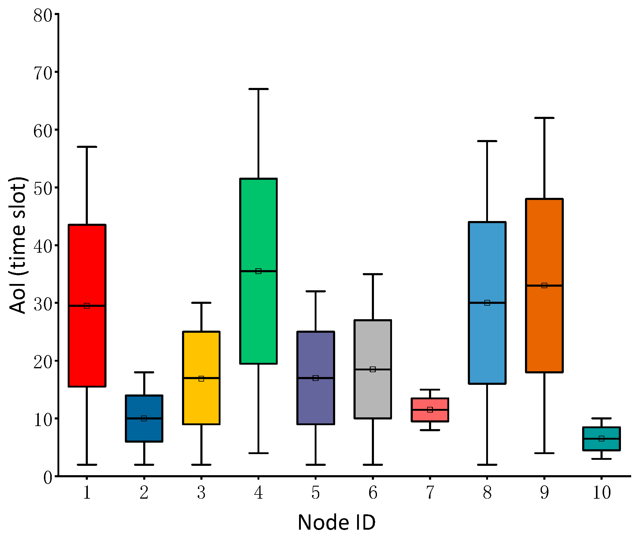
Figure 4 shows the real-time AoI, with the corresponding peak AoI and benchmark of the three representative nodes. Clearly, the AoI of all three nodes is below its corresponding peak AoI. The node’s peak AoI changes periodically, guaranteeing each node’s BAI. Under the proposed algorithm, since the peak AoI is positively correlated with $I_i$, it causes the maximum peak AoI of node 9 to be higher than the rest of the nodes, resulting in a greater BAI. The periodic variation of the AoI of nodes within the BAI interval can be attributed to the utilization of the floor function in determining the transmission interval of nodes in (8). As a result, the transmission period of nodes is shorter than the data generation period. Furthermore, the network employs a superframe-based periodic cycle scheduling method, which leads to the periodic variation of the time interval between node transmission slots and node sampling slots. In addition, we analyzed the AoI of all nodes and confirmed the BAI of all nodes and the peak AoI and average AoI of all ten sensor nodes, as shown in Figure 5.

In Figure 6, the effectiveness of reducing the peak AoI of a node by adjusting its TIC ${\alpha }_i$ is demonstrated, with node #9 used as an example. By adjusting the ${\alpha }_9$ of node #9 from 4 to 2 and 1, a reduction in the peak AoI of the node was observed. Decreasing the TIC can increase the number of transmission slots allocated to nodes. However, the TIC cannot be arbitrary, as a coefficient that is too small would reduce the network’s schedulability; the value of coefficient ${\alpha }_i$ must satisfy the constraint in (9).

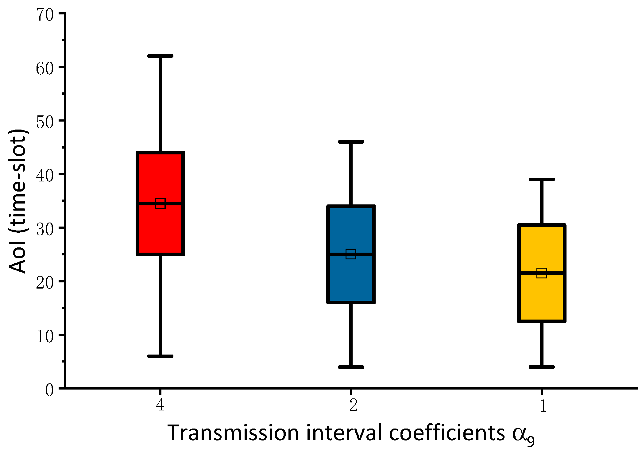
The boxplot of the AoI for node #9 with different ${\alpha }_9$ is shown in Figure 7, which indicates that reducing the TIC ${\alpha }_9$ leads to a decrease in the peak AoI, while the average AoI of the node also decreases accordingly.

To evaluate the schedulability of the proposed algorithm, we conducted experiments to test its scheduling success rate under varying numbers of nodes and average sampling periods, as shown in Figure 8. The scheduling success rate is defined as the percentage of test cases for which the algorithm is able to find a feasible schedule [30]. The scheduling success rate exhibits a decreasing trend with an increase in the number of nodes, which can be attributed to the requirement for additional time slots as the number of nodes increases. Similarly, a decrease in the average time sampling period leads to a reduction in the scheduling success rate. This can be attributed to the fact that a smaller sampling period results in an increased number of packets being sent within a single superframe.

5. Conclusions and Future Works

This paper proposed a scheduling algorithm guaranteeing each node’s AoI within a bounded interval in an IWSN where the sensor nodes’ sampling periods vary significantly, which is crucial for ensuring the stability of industrial systems. We determined the node’s transmission interval and superframe length according to the node’s sampling period to ensure network scheduling feasibility. Furthermore, we proposed a method to decrease the peak AoI by allocating more time slots for the nodes. A numerical example is given to illustrate the proposed algorithm step by step; the numerical results showed that the proposed algorithm could guarantee that the AoI of each node would be below the corresponding peak AoI.

In the future, the proposed algorithm is expected to be implemented in a real IWSN scheduler to test the AoI performance with real industrial data. Moreover, the algorithm can be extended to support multi-hop topology, while also taking into account lossy wireless channel models.