Article

A Robust Fault Diagnosis Scheme for Converter in Wind Turbine Systems

School of Astronautics, Northwestern Polytechnical University, Xi’an 710072, China
*
Authors to whom correspondence should be addressed.
Electronics 2023, 12(7), 1597; https://doi.org/10.3390/electronics12071597
Submission received: 11 March 2023 / Revised: 26 March 2023 / Accepted: 27 March 2023 / Published: 29 March 2023

Abstract

:
Fault diagnosis is a powerful tool to reduce downtime and improve maintenance efficiency; thus, the low management cost of wind turbine systems and effective utilization of wind energy can be obtained. However, the accuracy of fault diagnosis is extremely susceptible to the nonlinearity and noise in the measured signals and the varying operating conditions. This paper proposes a robust fault diagnosis scheme based on ensemble empirical mode decomposition (EEMD), intrinsic mode function (IMF), and permutation entropy (PE) to diagnose faults in the converter in wind turbine systems. Three-phase voltage signals output by the converter are used as the input of the fault diagnosis model and each signal is decomposed into a set of IMFs by EEMD. Then, the PE is calculated to estimate the complexity of the IMFs. Finally, the IMF-PE information is taken as the feature of the classifier. The EEMD addresses nonlinear signal processing and mitigates the effects of mode mixing and noise. The PE increases the robustness against variations in the operating conditions and signal noise. The effectiveness and reliability of the method are verified by simulation. The results show that the accuracy for 22 faults reaches about 98.30% with a standard deviation of approximately 2% under different wind speeds. In addition, the average accuracy of 30 runs for different noises is higher than approximately 76%, and the precision, recall, specificity, and F1-Score all exceed 88% at 10 dB. The standard deviation of all the evaluation indicators is lower than about 1.7%; this proves the stable diagnostic performance. The comparison with different methods demonstrates that this method has outstanding performance in terms of its high accuracy, strong robustness, and computational efficiency.

1. Introduction

The renewability and cleanness of wind energy render wind turbine systems sustainable solutions to meet the growing energy demand and mitigate the effects of greenhouse gas emissions [1]. Additionally, the flexible investment scale and short construction period of wind farms improve the power structure in rural areas and effectively solve agricultural electricity consumption [2]. The wind power system has developed rapidly in the past decade, and the global installed capacity has been increasing [3]. The global wind power accounted for 5% of global electricity production in 2021, which is on par with solar photovoltaic power generation, and is second only to hydropower in renewable energy generation [4], as shown in Figure 1.
Wind turbine systems are usually installed in coastal island, grassland, offshore, or remote areas. The high loads and the harsh environmental conditions, such as salt spray, extreme temperatures, and humidity, make the system more prone to failures. Therefore, reliability and maintenance costs are critical for the large-scale development of wind turbine systems. High reliability is conducive to its good operation, improving the effective utilization of wind energy [5]. The maintenance costs for onshore systems can reach up to 15% of the total cost, while those for offshore systems can reach up to 30% [6]. Fault diagnosis technology is taken as an effective tool to enhance the operation reliability and debase the maintenance costs [7,8].
A power converter is an important component in wind turbine systems. According to the statistics, the annual fault rate of wind power converters is as high as 17.5%, and its downtime percentage reached 14.3% [9]; thus, it is fragile. On the other hand, a non-recurring cost breakdown from the United Kingdom government shows that the replacement cost of a wind power converter is very expensive; the wind turbine system accounts for 33% of the total cost, of which the converter accounts for 8% [10]. Converter faults not only debase the power quality, but also cause damage to other components and endanger the power grid security, in turn increasing the production costs [11]. The high-accuracy fault diagnosis of the converter is essential for efficient fault-tolerant control and improving the converter operation capability under a fault state [12]. Furthermore, it enables operators to find faults as early as possible in order to take measures to avoid catastrophic accidents, and subsequently ensuring the safety of power production [13]. Moreover, it can help maintenance personnel quickly and accurately locate converter faults, improving maintenance efficiency, reducing maintenance costs, and increasing economic revenue [14].
Model-based approaches require the establishment of an accurate analytical model for the converter system using physical knowledge of the system structure and dynamics; then, the fault results are obtained by analyzing the residual between the estimation and the actual measurement. A sliding mode integral observer-based fault diagnosis method was proposed for multilevel converters open-circuit (OC) faults [15]. A nonlinear adaptive observer-based fault diagnosis method for a modular multilevel converter in a wind turbine system was proposed to obtain the online detection and location of OC faults [16]. The real-time fault diagnosis of a single-switch OC and a multi-switch OC of a converter were obtained based on the Kalman filter [17]. However, their diagnostic accuracy significantly relies on the precision of the system model and parameters. Signal-based approaches generate diagnostic variables and thresholds by studying the converter behaviors under different fault states in order to detect and locate faults. Inverter faults were diagnosed by detecting positive and negative sequence components [18]. A current trajectory fault diagnosis strategy was proposed to identify the converter faulty switch, reducing the effects of random wind speed [19]. The absolute normalized current and adaptive threshold were utilized to realize the real-time fault diagnosis of a wind converter [20]. However, they need prior knowledge of converter systems and are susceptible to thresholds.
Data-driven approaches are becoming popular because accurate converter models and prior-knowledge of the system are not necessary. They can diagnose faults only by mathematical analysis of a large number of system data. Fast Fourier transform (FFT) was used to extract the fault features [21], and then principal component analysis (PCA) was applied to obtain the low-dimensional features; finally, fault identification was performed using a relevance vector machine. An FFT-Relative PCA (RPCA)-support vector machine (SVM) scheme was presented for inverter fault diagnosis [22]. The FFT-PCA-Bayes networks (BNs) scheme was proposed to improve the robustness to bias and noise in converter measurement signals [23]. Discrete wavelet transform (DWT) was utilized to extract the detail coefficients of normalized currents as fault features, then the artificial neural network (ANN) was used for fault recognition of the inverter switch [24]. An DWT-approximate coefficient-energy vector was used as the fault feature [25]. DWT-PCA was presented to extract the fault features from the voltage signals of the inverter [26]. Feature analysis and judgment were performed on the signal processed by wavelet transform (WT) [27], then the back propagation neural network (BPNN) was used to identify OC faults in the wind power converter. The principal component energy value and proportional coefficient of the forward current of each phase are used to construct fault features to locate the faulty leg in the inverter [28]. The normalized average currents were used to generate diagnostic variables, then the fuzzy logic system (FLS) was used to identify the inverter faulty switch [29]. Concordia transform and random forests were used to diagnose switch OC faults [30]. Predictive current errors were combined with FLS for power switch fault diagnosis [31].
It should be noted that feature extraction is crucial for data-driven approaches, and effective feature representation can significantly improve the accuracy of the fault diagnosis. In fact, the fault diagnosis performance greatly depends on the feature extraction technique. However, the nonlinearity and instability of the wind power converter signal make FFT and WT unable to guarantee the diagnostic accuracy because FFT produces error information for nonlinear signals and has no time resolution; WT is susceptible to wavelet basis functions and is non-adaptive. In addition, feature representation, such as detail coefficients, approximate coefficient, energy vector, Concordia transform, and predictive current errors, are susceptible to loads, operating conditions, and noise. The application of the signal denoising technique is an effective scheme to improve the diagnostic accuracy [32], but the complexity of the diagnostic method increases accordingly.
The topology and configuration of wind power converters continue to evolve due to the constant emergence of complex high-power machinery. In addition, wind power converters suffer from numerous stresses and operating condition variations. Therefore, it is necessary to develop an intelligent fault diagnosis strategy for wind power converters to meet the requirements of intelligent maintenance and management that does not require accurate system model and prior knowledge of signal patterns. In addition, this method should have high reliability and strong robustness, which is essential for practical engineering applications. The nonlinearity and non-stationarity of wind power converter signals make it significant to develop a fault diagnosis strategy that can deal with the nonlinearity and non-stationarity in the signal.
This paper presents a robust adaptive data-driven intelligent fault diagnosis scheme ensemble empirical mode decomposition (EEMD)-permutation entropy (PE) for power converters in wind turbine systems. EEMD was used to decompose nonlinear and non-stationary three-phase voltage signals of a converter into a set of intrinsic mode functions (IMF). Then, the PE is calculated to estimate the complexity of the IMFs, and the IMF-PE is taken as the feature of the classifier. The reliability and robustness of the method to wind speed and noise are further studied. The main contributions are:
  • EEMD realizes the adaptive processing of nonlinear and non-stationary signals, and its application mitigates mode mixing and the effects of noise interference;
  • The complexity measure of PE enhances the robustness against variations in the operating conditions and signal noise;
  • IMF-PE highlights the signal local characteristics;
  • The effects of the embedding dimension on the fault diagnosis results are studied, and the optimal value is selected;
  • The scheme has high reliability and robustness and low time consumption. It also has a stable diagnostic performance.
The rest of this paper is organized as below: Section 2 describes a back-to-back converter in a doubly fed wind power system, then analyzes its fault modes and the reliability and robustness issues to be considered. Section 3 proposes a robust intelligent fault diagnosis scheme: EEMD-PE. Section 4 establishes the simulation model and gives rigorous comparative analyses. Section 5 concludes with several remarks.

2. Fault Analysis and Diagnostic Requirements for Wind Power Converter

2.1. Fault Analysis

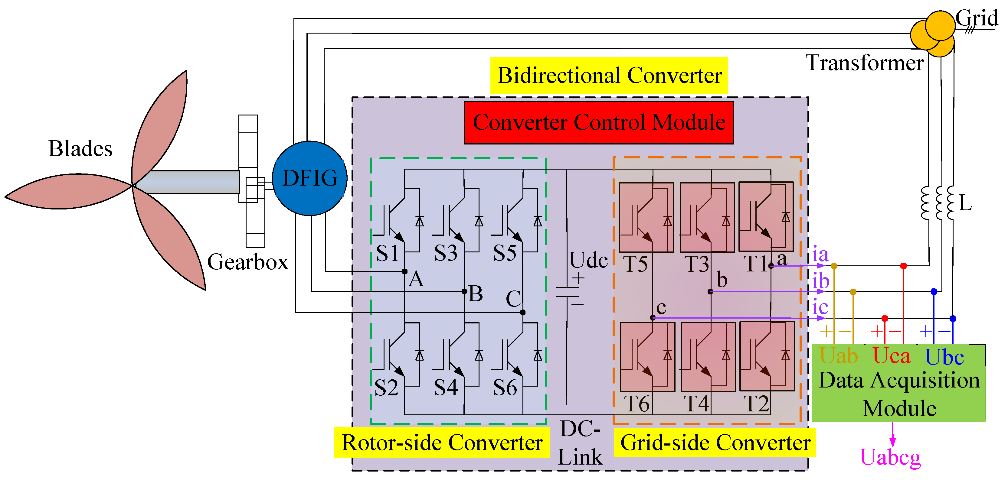
The topology of a doubly fed induction generator (DFIG) wind turbine system is shown in Figure 2. The main components of the system are the blades, gearbox, generator, back-to-back converter, and control system. The back-to-back converter consists of a rotor-side converter and a grid-side converter. The rotor-side converter tracks the maximum wind energy, thus improving the system operation efficiency. The grid-side converter keeps U d c constant and prevents grid-side current harmonics. They have the same structure, and contain three-phase bridge arms with six insulated gate bipolar transistor (IGBT) power switches. Each switch is controlled by a gate signal; it is turned on when the gate signal equal to 1 and turned off when the gate signal equal to 0.
Converter faults can be divided into short-circuit (SC) faults and open-circuit (OC) faults. SC faults are easy to detect because they usually produce an abnormal overcurrent and cause system protection. OC faults respond slowly and do not cause the system to collapse immediately. However, they can cause a high harmonic in the currents, and cause current offset in the healthy phase and the faulty phase, resulting in generator torque oscillation and grid power factor reduction. Moreover, long-term OC fault operation can damage the generators and capacitors. In addition, SC faults will eventually turn into OC faults due to the action of the circuit breakers and fuses. Thus, when an OC fault occurs in the power converter, the operational safety of the wind turbine system can be significantly affected, and the power production is reduced. Therefore, OC fault diagnosis is necessary for earlier faults decision and risk reduction.
The internal fault mechanisms of the IGBT open circuit mainly include gate drive faults and thermal stresses. The external fault mechanisms of the IGBT open circuit mainly include bond wire lift-off, bond wire rupture, cracking of solder layers, and the drive board open circuit. These fault mechanisms will ultimately manifest as IGBT OC faults. Different IGBT OC faults constitute different fault modes. For a grid-side converter, there are 22 fault modes: when six switches are healthy, that is the normal state; when only one switch is faulty, six fault modes are formed, namely T1, T2, T3, T4, T5, T6; when the upper and lower switches of the same bridge arm fail at the same time, three fault modes are formed, namely T1 and T2, T3 and T4, T5 and T6; when two switches of the same half-bridge are faulty, six fault modes are formed, namely T1 and T3, T1 and T5, T3 and T5, T2 and T4, T2 and T6, T4 and T6; when the simultaneous fault of two switches of different half-bridges occurs, six fault modes are formed, namely T1 and T4, T1 and T6, T3 and T2, T3 and T6, T5 and T2, T5 and T4. The fault diagnosis of single and dual-IGBT OC faults is studied as it is rare for three or more IGBTs to fail simultaneously. The input signal selection of the fault diagnosis model directly affects the diagnostic accuracy. In the wind turbine system, the output voltage signals Uab, Ubc, and Uca are constant with the load variation, while the current signals ia, ib, and ic are easily affected. Therefore, the three-phase voltage signals are selected as the input to the diagnosis method.

2.2. Diagnostic Requirements

The mass configuration of nonlinear power switches and the complex working conditions make the output signals of the wind power converter nonlinear and non-stationary; thus, the reliability of the fault diagnosis method for the converter requires superior processing capability for nonlinear and non-stationary signals. The wind turbine system involves high dynamics, rapid changes in the wind speed and frequent changes in the grid load cause abrupt changes in the torque, so the fault diagnosis method for the power converter should have strong robustness to wind speed and load. Additionally, the signals measured by the sensors contain noise, which has a serious impact on the diagnostic accuracy; thus, the proposed fault diagnosis method should be robust to noise.

3. Fault Diagnosis Method

3.1. The Proposed Fault Diagnosis Method

This section describes in detail the presented fault diagnosis method EEMD-PE to diagnose OC faults of wind power converters. The diagnosis steps are as follows:
  • Acquiring three-phase line-to-line voltages Uabcg (Uab, Ubc, Uca) from simulation under both healthy and faulty operating condition, then using them as fault signals to train and test the proposed fault diagnosis method;
  • Decomposing each fault signal into a group of IMFs using EEMD;
  • Obtain the minimum number of all IMFs of all fault signals and noted as ;
  • Calculating the PE of each IMF as a fault feature to reflect the complexity of the signal. The IMF-PE feature is expressed as:
    H P E = [ H P E ( IMF 1 / U ab ) , H P E ( IMF 2 / U ab ) , , H P E ( IMF / U ab ) , H P E ( IMF 1 / U bc ) , H P E ( IMF 2 / U bc ) , , H P E ( IMF / U bc ) , H P E ( IMF 1 / U ca ) , H P E ( IMF 2 / U ca ) , , H P E ( IMF / U ca ) ]
  • Diagnosing the faults using SVM. The fault features are marked as fault labels and further randomly divided into training samples and testing samples, and the ratio of training samples to testing samples is set as 3:2.

3.2. Signal Decomposition Using EEMD

Empirical mode decomposition (EMD) is a data-driven adaptive signal processing technique for nonlinearity and non-stationary signals [33]. It decomposes a complex signal into a group of simple oscillation modes based on the local feature time scale of the signal, namely, the intrinsic mode functions (IMFs). An IMF satisfies the EMD conditions and sifting stop criteria [34], and it is produced by an algorithm rather than a specified kernel function. Ensemble empirical mode decomposition (EEMD) is a noise assisted EMD algorithm implemented by performing EMD over the ensemble of signal plus noise [35]. It can not only mitigate mode mixing in the EMD, but is also robust to noise. The IMFs of EEMD are obtained by adding white noise to the original signal and averaging the EMD decomposition results.
For a signal x ( t ) , the steps of the EMD algorithm and EEMD algorithm are described in Table 1 and Table 2, respectively. The block diagrams of the EMD algorithm and EEMD algorithm are shown in Figure 3.
After the EMD decomposition procedure is ended, a set of IMFs ( d 1 , d 2 , , d I ) and a residue r I are obtained, and x ( t ) = i = 1 I d i + r I , where ( d 1 , d 2 , , d I ) contains different signal frequencies, from high to low, r I represents the average trend of x ( t ) .

3.3. Feature Extraction Using PE

Permutation entropy (PE) can quantify the dynamics and uncertainties of the time series, and is quite sensitive to changes in nonlinear signals, so it can be treated as a powerful tool for the complexity measurement of nonlinear signals [36]. Due to the simple calculation, short time consumption, good real-time performance, and strong robustness to noise, PE is used to extract the feature information from the fault signal of the converter. The PE estimates the complexity of the signal by comparing the neighboring values. For a given signal u ( n ) = { u ( 1 ) , u ( 2 ) , , u ( N ) } , the PE is calculated as follows:
Step 1.
Reconstruct the phase space of the signal, and each subsequence is represented as X ( i ) , then the results can be obtained:
X ( i ) = { u ( i ) , u ( i + τ ) , , u ( i + ( m 1 ) τ ) }               i = 1 , 2 , , N ( m 1 ) τ
where, m is the embedding dimension, τ is the time delay.
Step 2.
Rearrange each X ( i ) in ascending order:
u ( i + ( j 1 1 ) τ ) u ( i + ( j 2 1 ) τ ) u ( i + ( j m 1 ) τ )
where j 1 , j 2 , , j m is the location index of the elements in X ( i ) after reordering. If two values are equal, they are sorted according to the value of j η . In this way, each X ( i ) is mapped to a symbol sequence:
λ ( s ) = ( j 1 , j 2 , , j m )
which is one of the m ! permutations, and s = 1 , 2 , , k , k m ! .
Step 3.
The probability distribution of all the symbol sequences is expressed as P 1 , P 2 , , P k , and P k is defined as:
P k = f ( k ) N ( m 1 ) τ
where f ( k ) is the occurrence times of the k-th symbol sequence.
Step 4.
PE is defined as:
H ( m , τ ) = j = 1 k P j ln P j
when P j = 1 m ! , there is no repetition in the symbol sequence, the signal complexity is the highest and PE obtains the maximum, which is ln ( m ! ) .
It should be noted that m and τ are two major parameters affecting the PE. If m is too small, the permutation space will be very small, resulting in a few different states, so the scheme is invalid; in theory, it is better to take the larger value of m, as long as the length of the signal is proportional to m ! . However, the larger the m is, the higher the computational complexity and the more time-consuming it will be. The purpose of the research is to detect the changes in the signal, so it is inappropriate for m to be too large. In addition, the value of τ is required to be greater than or equal to 1.

4. Simulation Results and Discussion

4.1. Simulation Platform

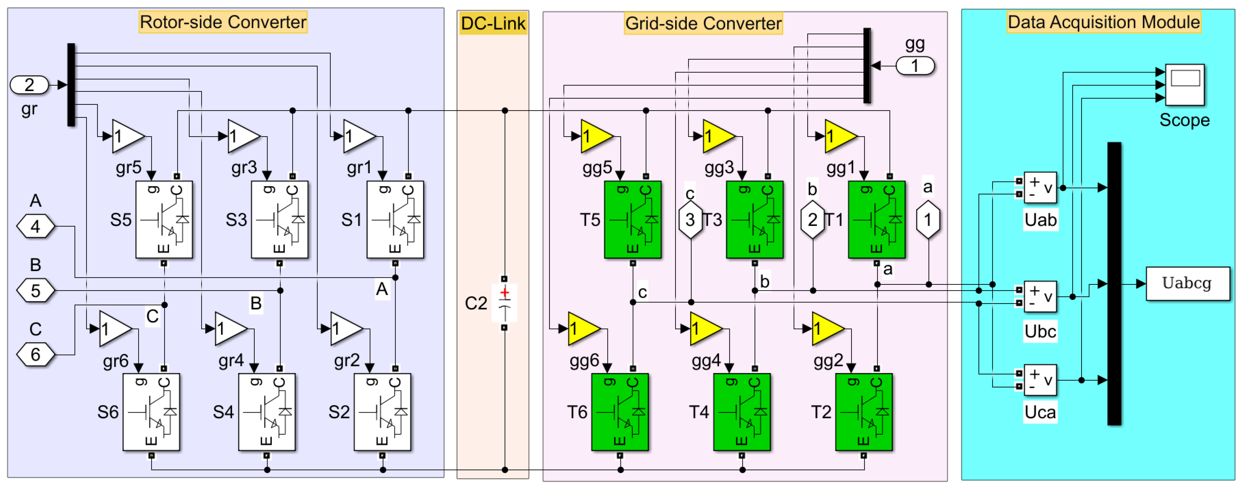
In order to evaluate the performance of the proposed fault diagnosis scheme, EEMD-PE, the DFIG wind power system simulation model is established using MATLAB software, and the converter model is shown in Figure 4. Some of the main parameters are shown in Table 3.
The IGBT OC fault is obtained by removing the corresponding gate signal, for example, an OC fault is inserted into T1 by setting the gain gg1 to 0. Measure the three-phase line-to-line voltage Uabcg (Uab, Ubc, Uca) of the converter under different fault states; the results are shown in Figure 5, and it can be seen that the OC fault in the switch can cause the distortion of the Uab, Ubc, and Uca signals, so the converter fault modes can be identified by analyzing the Uab, Ubc, and Uca signals.
Sample for 1 s and the sampling frequency is 10 kHz, so the size of sample is 10,000. For assessing the robustness to wind speed changes of the proposed fault diagnosis scheme, the voltage signals Uab, Ubc, and Uca of the converter are measured when the wind speed changes from 10 m/s to 15 m/s with the interval of 0.0625 m/s. Thus, there are 81∗3∗22 = 5346 samples in 22 fault modes.

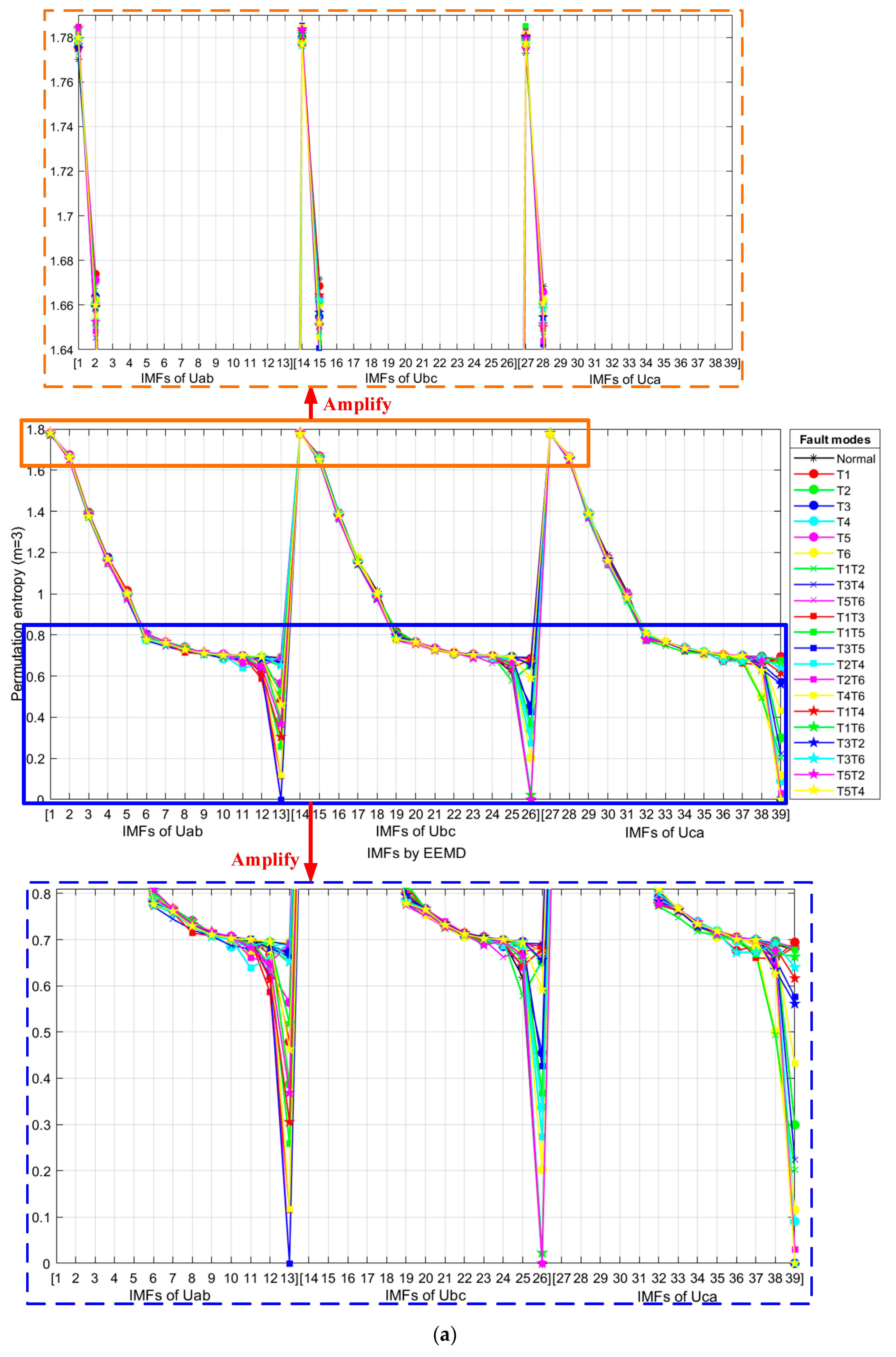
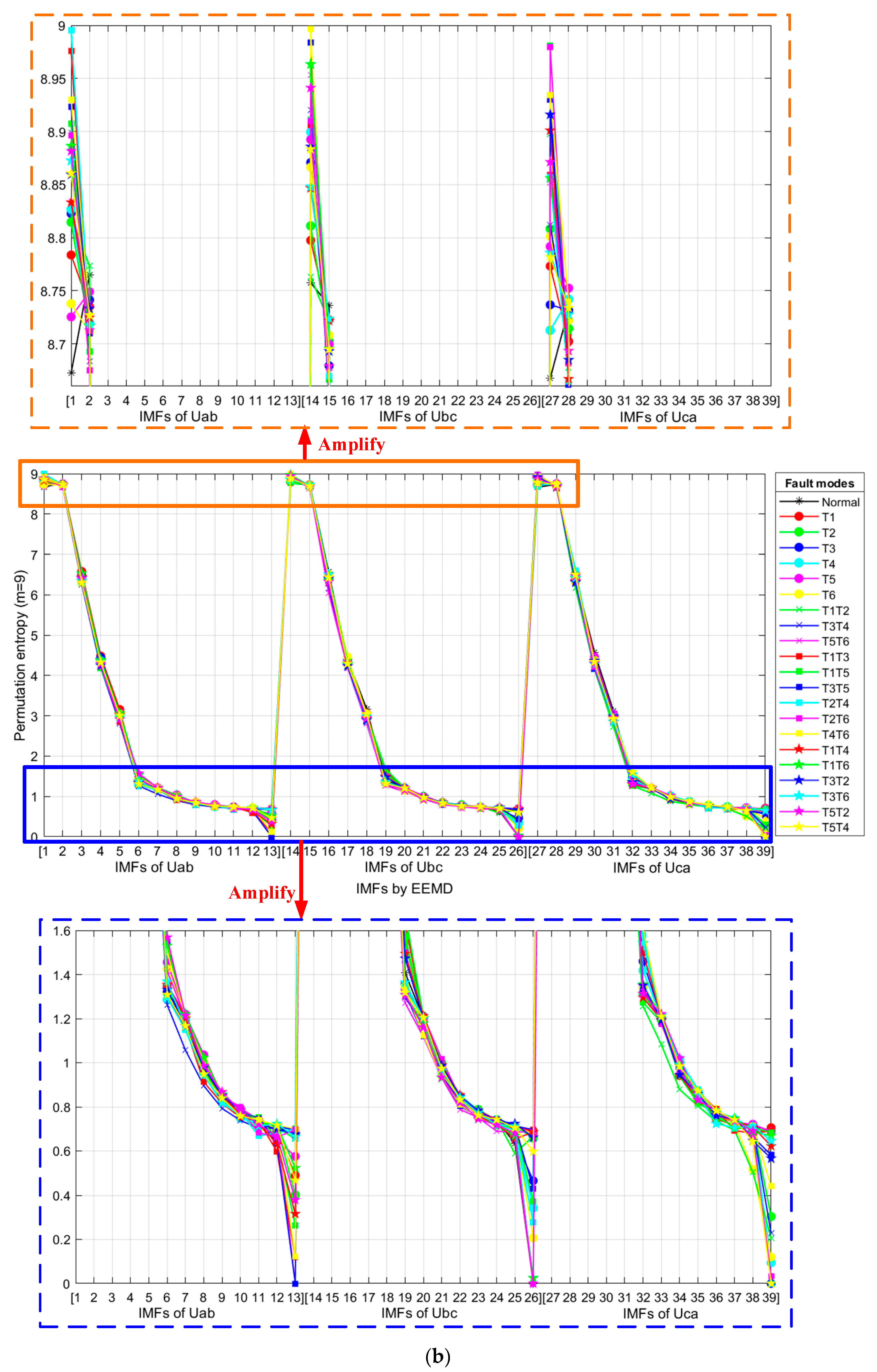
4.2. Results of EEMD-IMF-PE Feature

For the 22 fault modes, the PE calculation results of the EEMD-IMFs with different embedding dimensions m are shown in Figure 6 (set time delay τ = 1). In addition, the local results are amplified for the convenience of comparison. It can be seen from Figure 6 that the PE values of IMF1 in different fault modes are significantly different when m = 9, while they are similar when m = 3, and the results have the same phenomenon for IMF2, IMF14, IMF15, IMF27, and IMF28. In addition, the PE values of IMF6-IMF13 (IMF19-IMF26, and IMF32-IMF39) in different fault modes have a more significant difference when m = 9 than when m = 3. Therefore, the PE feature with a large value of m is superior for distinguishing different converter fault modes.

4.3. Results of Classification

In order to analyze the effects of the embedding dimension m on the fault diagnosis results, the comparison of the SVM classification results is presented under different values of m. First, 10 dB and 20 dB white noise is added into the voltage signal with different wind speeds, respectively. The training samples and testing samples are randomly divided, and the training-to-testing ratio is 3:2. The value of m changes from 3~9, and the set time delay τ = 1. The effects of m on the average accuracy of 30 runs are shown in Figure 7a, and the effects of m on the calculation time of the PE are shown in Figure 7b. In order to show the results more clearly, the specific coordinate values of the curves are shown in Figure 7a,b. Since the calculation time of PE is close at 10 dB and 20 dB, only the specific coordinate value of the curve at 10 dB is shown in Figure 7b.
As shown in Figure 7a, the diagnostic accuracy is significantly improved with the increase in m, and the improvement becomes not obvious when m exceeds 6. It can be seen from Figure 7b that the larger the value of m, the longer the calculation time of PE, and the calculation time increases greatly when m exceeds 6. In particular, for 10 dB, the PE calculation time under m = 9 is 121 times longer than that under m = 6 (53.4/0.44 = 121), but the diagnostic accuracy under m = 9 is only 0.51% higher than that under m = 6 (88.63 − 88.12 = 0.51); in addition, Figure 7b is only a comparison of the calculation time for the Uab of a normal state, so the time consumption for all samples 22∗3∗81 = 5346 is extremely heavy in m = 9; thus, m = 9 is uneconomical. Similarly, the diagnostic accuracy under m = 7 is only 0.13% higher than that under m = 6, while the calculation time is increased by about 5 times.
In order to evaluate the stability of the method, the diagnosis results of 22 faults at 20 dB noise under different m values are shown in Table 4, and the average value and standard deviation are also provided.
As shown in Table 4, the average accuracy of 22 faults at m = 5 (97.8693%) is significantly higher than that at m = 3 (94.0341%) and m = 4 (95.5966%). When m is greater than 6, the average accuracy gradually increases, but the increase is not obvious. In addition, when m exceeds 6, the standard deviation of the accuracy of the 22 faults can be maintained at about 2%, which is significantly lower than 6.8131% at m = 3, 5.2521% at m = 4, and 3.9039% at m = 5. As a result, when m exceeds 6, high diagnostic accuracy can be obtained, and the diagnostic results have a more stable performance.
In summary, the calculation time of PE increases exponentially after m exceeds 7, while the diagnostic accuracy and stability performance are already quite high at m = 6. Thus, it is effective and economical to select m as 6. Therefore, when m = 6, the proposed fault diagnosis method has an outstanding performance in terms of its high accuracy, high stability, and low time consumption.

4.4. Analysis of Robustness

The classification results are presented with different wind speeds to assess the robustness of the proposed method to wind speed: 20 dB, 15 dB, 10 dB, and 5 dB white noise is added into the voltage signal at different wind speeds, respectively. Set the embedding dimension m = 6 and time delay τ = 1. The training samples and testing samples are randomly divided as 3:2. Running 30 times, the results of some of the evaluation indicators (accuracy, precision, recall, F1-Score, specificity, false alarm rate (FAR), and missing alarm rate (MAR)) of the proposed method for all noise conditions are recorded, as shown in Table 5, including the minimum, maximum, average, and standard deviation.
From Table 5, for 20 dB, the average diagnostic accuracy can reach 97.8220%, and the standard deviation of accuracy for 30 runs is 0.5735%, so the proposed method has an excellent ability to classify the overall samples correctly and has a stable performance. Furthermore, the high average precision (97.9108%) and high average recall (97.8220%), respectively, reflect the outstanding ability to correctly predict positive samples and the effectiveness of the method to identify positive labels. The low standard deviation of the precision (0.5387%) and low standard deviation of the recall (0.5735%) indicate the stability of the diagnostic performance. The F1-Score is the harmonic mean of the precision and recall to balance the single-dimensional metrics defects of the two indicators, and it achieves a 97.8186% high performance, and the standard deviation is only 0.5756%. Its high average specificity (99.8963%) and its low standard deviation (0.0273%) indicate that this method can stably and correctly predict negative samples. In addition, the average FAR (0.1037%) and average MAR (2.1780%) are also very low, with small standard deviations. These results show that the proposed fault diagnosis method can accurately and stably diagnose switch faults at 20 dB signal noise; therefore, it has an excellent robustness to wind speed changes.
It also can be seen from Table 5 that the average accuracy for all noises is higher than about 76%, and it reaches 88.1203% at 10 dB and 96.3021% at 15 dB. In addition, its average precision, average recall, and average F1-Score all exceed 88% at 10 dB, and the average specificity even exceeds 99%. The average FAR and average MAR for all noises are below about 0.5% and 11%, respectively. Thus, this method has strong noise robustness. In addition, the standard deviation of all the evaluation indicators for all noises is lower than about 1.7%, so this method has a stable diagnostic performance for all noises.
To summarize, this method not only has strong robustness to wind speed, but also has an excellent and stable performance in the noise environment.

4.5. Comparison of Different Methods

This section compares the proposed fault diagnosis method, EEMD-PE, with different methods to prove the excellence of the proposed method. The different methods are compared in Figure 8 to highlight the advantages of EEMD, including EEMD-PE, EMD-PE, complete ensemble empirical mode decomposition with adaptive noise (CEEMDAN)-PE [37], improved complete ensemble empirical mode decomposition with adaptive noise (ICEEMDAN)-PE [38], and direct PE feature extraction (represented as direct PE). The diagnostic accuracies (average of 30 running) of the different methods are shown in Figure 8a, and the calculation times of the different methods are shown in Figure 8b.
As shown in Figure 8a, although the diagnostic accuracy of the direct PE method exceeds 60% at 20 dB, it is not satisfactory at other noise levels (15 dB, 10 dB, 5 dB), indicating that the PE feature can represent the converter fault modes, but is highly susceptible to signal noise. In addition, the accuracy of the EEMD-PE method, the CEEMDAN-PE method, and the ICEEMDAN-PE method is significantly more improved than that of the EMD-PE method and the direct PE method, indicating that the EEMD, CEEMDAN, and ICEEMDAN algorithms not only overcome the disadvantage of the mode mixing of EMD, but also has strong robustness to signal noise. It also can be seen from Figure 8a that the accuracy of the EEMD-PE method is the highest, which is close to 90% at 10 dB and 100% at 20 dB; in addition, the decomposition time of EEMD is significantly lower than that of CEEMDAN and ICEEMDAN at all noise levels, as shown in Figure 8b, and this is only a comparison of the decomposition time for the Uab of a normal state, so CEEMDAN and ICEEMDAN are time-consumption heavy for all 5346 samples. The results show that the EEMD-PE method not only has the highest diagnostic accuracy, but also consumes less time. Thus, the EEMD-PE method is optimal.
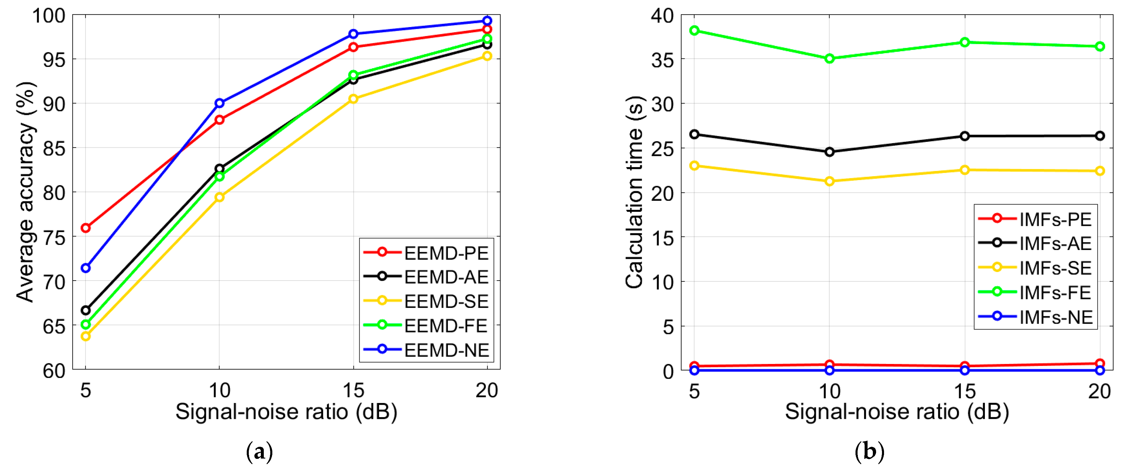
The different methods are compared in Figure 9 to highlight the advantages of PE, including EEMD-PE, EEMD-approximate entropy (AE), EEMD-sample entropy (SE), EEMD-fuzzy entropy (FE), and EEMD-norm entropy (NE) [11]. The diagnostic accuracies (average of 30 running) of the different methods are shown in Figure 9a, and the calculation times of the different methods are shown in Figure 9b.
From Figure 9a, the diagnostic accuracy of the EEMD-PE method and the EEMD-NE method are both above about 95% (15 dB) and 70% (5 dB), significantly higher than that of the EEMD-AE method, EEMD-SE method and EEMD-FE method. Figure 9b shows that the calculation of the IMFs-PE feature and IMFs-NE feature is very fast, and the calculation time is much lower than that of the IMFs-FE feature, IMFs-AE feature, and IMFs-SE feature. It should be noted that this is only a comparison of the calculation time for the Uab of a normal state, so the calculation speed of the IMFs-PE feature and IMFs-NE feature is perfect for all 5346 samples. Therefore, the performance of the EEMD-PE method and EEMD-NE method is better than that of the EEMD-AE method, EEMD-SE method and EEMD-FE method. In addition, the diagnostic accuracy of the EEMD-PE method (75%) is higher than that of the EEMD-NE method (70%) for the signal-to-noise ratio of 5 dB. Therefore, the EEMD-PE method is more suitable for the high-noisy environment than the EEMD-NE method.
In summary, the accuracy of the EEMD-PE method is optimal at all noise levels, and the accuracy is acceptable; additionally, its calculation speed is fast. These results show that the EEMD-PE method is preferred in terms of accuracy, robustness to noise, and time consumption.

4.6. Comparison with Previous Schemes

In order to highlight the advantages of the proposed scheme, it is compared with similar ones in the literature, as shown in Table 6. The average accuracy and standard deviation of the accuracy under different noise conditions are provided to highlight the high robustness and stability of the proposed scheme. In order to prove the fairness of the comparison, the diagnostic fault types, training to testing ratio, and the number of runs of each scheme are also given in Table 6.
From Table 6, the diagnostic average accuracy of the EEMD-PE scheme in 20 dB (97.8220%) and in 10 dB (88.1203%) are all higher than that of the MEMD-FE scheme [12] in 20 dB (92.1477%) and in 10 dB (84.2338%), indicating that the EEMD-PE scheme has stronger robustness to noise than MEMD-FE scheme. In addition, the standard deviation of the accuracies for the EEMD-PE scheme in 20 dB (0.5735%) and in 10 dB (1.0354%) are significantly lower than that of the MEMD-FE scheme [12] in 20 dB (1.3312%) and in 10 dB (1.7167%); thus, the EEMD-PE scheme is more stable than the MEMD-FE scheme. Although the average accuracy of the EEMD-PE scheme is slightly lower than that of the EEMD-NE scheme [11] at 20 dB, 15 dB, and 10 dB, it is significantly higher at 5 dB (75.9375%) than that of the EEMD-NE scheme at 5 dB (71.8040%). As a result, the EEMD-PE scheme is more robust to large noise than the EEMD-NE scheme, and is more suitable for applications in large noise environments.

4.7. Discussion

This scheme is a data-driven fault diagnosis technology that requires only a large amount of data. It diagnoses faults through mathematical techniques, facilitating transplantation to other topics. As analyzed above, this scheme is suitable for processing nonlinear and non-stationary signals and has strong robustness and stability against large noise. This characteristic makes this scheme very suitable for applications in large noise and nonlinear situations, such as mechanical fault diagnosis.

5. Conclusions

A robust fault diagnosis scheme based on ensemble empirical mode decomposition (EEMD), the intrinsic mode function (IMF), and permutation entropy (PE) is proposed in this paper for converter fault diagnosis in wind turbine systems. Three-phase voltages are used as the input of the fault diagnosis model. The effects of the embedding dimension m on the fault diagnosis results are studied, and the optimal m is selected. The EEMD algorithm addresses nonlinear signal processing in wind power systems and improves the robustness to wind speed changes, and the accuracy can reach approximately 98.30% at 20 dB; additionally, the precision, recall, F1-Score, specificity, FAR and MAR all have excellent performance when in variable wind speed. The diagnostic accuracy exceeds approximately 76% at 5 dB as the PE estimates the complexity of the fault signal and increases the robustness against signal noise. The standard deviation of all the evaluation indicators for different noises lower than about 1.7% demonstrates that the method has good stability. In addition, the scheme has low computation and time consumption and is suitable for real-time applications. Through the full demonstration and comparison of the different methods, this scheme is more suitable for high-noisy environments and real-time applications, so it is more available for practical applications.
For future study, it will be interesting to further analyze the fault features of power converters in wind turbine systems and explore more reliable and robust feature extraction methods under more realistic working conditions.

Author Contributions

Conceptualization, J.L.; methodology, J.L.; software, J.L.; validation, J.L.; formal analysis, J.L.; investigation, J.L. and K.Z.; resources, K.Z.; data curation, J.L.; writing—original draft preparation, J.L.; writing—review and editing, J.L.; visualization, J.L.; supervision, K.Z.; project administration, K.Z.; funding acquisition, K.Z. All authors have read and agreed to the published version of the manuscript.

Funding

This research received no external funding.

Data Availability Statement

Not applicable.

Conflicts of Interest

The authors declare no conflict of interest.

References

  1. Papadopoulos, P.; Coit, D.W.; Ezzat, A.A. Seizing Opportunity: Maintenance Optimization in Offshore Wind Farms Considering Accessibility, Production, and Crew Dispatch. IEEE Trans. Sustain. Energy 2022, 13, 111–121. [Google Scholar] [CrossRef]
  2. Javidsharifi, M.; Pourroshanfekr, H.; Kerekes, T.; Sera, D.; Guerrero, J. Stochastic Optimal Strategy for Power Management in Interconnected Multi-Microgrid Systems. Electronics 2022, 11, 1424. [Google Scholar] [CrossRef]
  3. Yang, L.; Li, G.; Zhang, Z.; Ma, X.; Zhao, Y. Operations & Maintenance Optimization of Wind Turbines Integrating Wind and Aging Information. IEEE Trans. Sustain. Energy 2021, 12, 211–221. [Google Scholar]
  4. REN21. Renewables 2022 Global Status Report. Available online: https://www.ren21.net/wp-content/uploads/2019/05/GSR2022_Full_Report.pdf (accessed on 23 March 2023).
  5. Saidi, L.; Benbouzid, M. Prognostics and Health Management of Renewable Energy Systems: State of the Art Review, Challenges, and Trends. Electronics 2021, 10, 2732. [Google Scholar] [CrossRef]
  6. Guo, Y.; Sheng, S.; Phillips, C.; Keller, J.; Veers, P.; Williams, L. A methodology for reliability assessment and prognosis of bearing axial cracking in wind turbine gearboxes. Renew. Sustain. Energy Rev. 2020, 127, 109888. [Google Scholar] [CrossRef]
  7. Li, S.; Cao, B.; Cui, Y.; Kang, Y.; Gao, S.; Li, H.; Dong, H. Terahertz-Based Insulation Delamination Defect Inspection of Vehicle Cable Terminals. IEEE Trans. Transp. Electrif. 2023, 9, 1765–1774. [Google Scholar] [CrossRef]
  8. Li, S.; Cao, B.; Kang, Y.; Cui, Y.; Dong, H. Nonintrusive Inspection of Moisture Damp in Composited Insulation Structure Based on Terahertz Technology. IEEE Trans. Instrum. Meas. 2021, 70, 10. [Google Scholar] [CrossRef]
  9. Liang, J.; Zhang, K.; Durra, A.A.; Muyeen, S.M.; Zhou, D. A state-of-the-art review on wind power converter fault diagnosis. Energy Rep. 2022, 8, 5341–5369. [Google Scholar] [CrossRef]
  10. Johnston, B.; Foley, A.; Doran, J.; Littler, T. Levelised cost of energy, A challenge for offshore wind. Renew. Energy 2020, 160, 876–885. [Google Scholar] [CrossRef]
  11. Liang, J.; Zhang, K.; Durra, A.A.; Zhou, D. A novel fault diagnostic method in power converters for wind power generation system. Appl. Energy 2020, 266, 114851. [Google Scholar] [CrossRef]
  12. Liang, J.; Zhang, K. A New Hybrid Fault Diagnosis Method for Wind Energy Converters. Electronics 2023, 12, 1263. [Google Scholar] [CrossRef]
  13. Mahdhi, H.B.; Azza, H.B.; Jemli, M. Experimental investigation of an open-switch fault diagnosis approach in the IGBT-based power converter connected to permanent magnet synchronous generator-DC system. Int. Trans. Electr. Energ. Syst. 2020, 30, 12436. [Google Scholar]
  14. Li, S.; Cao, B.; Li, J.; Cui, Y.; Kang, Y.; Wu, G. Review of condition monitoring and defect inspection methods for composited cable terminals. High Volt. 2023. early access. [Google Scholar] [CrossRef]
  15. Mtepele, K.O.; Campos-Delgado, D.U.; Valdez-Fernández, A.A.; Pecina-Sánchez, J.A. Model-based strategy for open-circuit faults diagnosis in n-level CHB multilevel converters. IET Power Electron. 2019, 12, 648–655. [Google Scholar] [CrossRef]
  16. Liu, H.; Ma, K.; Loh, P.C.; Blaabjerg, F. Online fault identification based on an adaptive observer for modular multilevel converters applied to wind power generation systems. Energies 2015, 8, 7140–7160. [Google Scholar] [CrossRef] [Green Version]
  17. Naseri, F.; Schaltz, E.; Lu, K.; Farjah, E. Real-time open-switch fault diagnosis in automotive permanent magnet synchronous motor drives based on kalman filter. IET Power Electron. 2020, 13, 2450–2460. [Google Scholar] [CrossRef]
  18. Al-Gahtani, S.F.; Azazi, H.Z.; Nelms, R.M.; Elbarbary, Z.M. Detection of negative sequence components in diagnosing and tolerating open-gate fault for a voltage-source inverter in an induction motor drive. IET Power Electron. 2020, 13, 4194–4203. [Google Scholar] [CrossRef]
  19. Qiu, Y.; Jiang, H.; Feng, Y.; Cao, M.; Zhao, Y.; Li, D. A new fault diagnosis algorithm for PMSG wind turbine power converters under variable wind speed conditions. Energies 2016, 9, 548. [Google Scholar] [CrossRef]
  20. Zhao, H.; Cheng, L. Open-circuit faults diagnosis in back-to-back converters of DF wind turbine. IET Renew. Power Gener. 2017, 11, 417–424. [Google Scholar] [CrossRef]
  21. Wang, T.; Xu, H.; Han, J.; Elbouchikhi, E.; Benbouzid, M.E. Cascaded H-bridge multilevel inverter system fault diagnosis using a PCA and multiclass relevance vector machine approach. IEEE Trans. Power Electron. 2015, 30, 7006–7018. [Google Scholar] [CrossRef]
  22. Wang, T.; Qi, J.; Xu, H.; Wang, Y.; Liu, L.; Gao, D. Fault diagnosis method based on FFT-RPCA-SVM for cascaded-multilevel inverter. ISA Trans. 2016, 60, 156–163. [Google Scholar] [CrossRef]
  23. Cai, B.; Zhao, Y.; Liu, H.; Xie, M. A data-driven fault diagnosis methodology in three-phase inverters for PMSM drive systems. IEEE Trans. Power Electron. 2017, 32, 5590–5600. [Google Scholar] [CrossRef]
  24. Dhumale, R.B.; Lokhande, S.D. Neural network fault diagnosis of voltage source inverter under variable load conditions at different frequencies. Measurement 2016, 91, 565–575. [Google Scholar] [CrossRef]
  25. Wu, F.; Hao, Y.; Liu, J.Z.Y. Current similarity based open-circuit fault diagnosis for induction motor drives with discrete wavelet transform. Microelectron. Reliab. 2017, 75, 309–316. [Google Scholar] [CrossRef]
  26. Gomathy, V.; Selvaperumal, S. Fault detection and classification with optimization techniques for a three-phase single-inverter circuit. J. Power Electron. 2016, 16, 1097–1109. [Google Scholar] [CrossRef] [Green Version]
  27. Zhang, J.; Sun, H.; Sun, Z.; Dong, W.; Dong, Y. Fault Diagnosis of Wind Turbine Power Converter Considering Wavelet Transform, Feature Analysis, Judgment and BP Neural Network. IEEE Access 2019, 7, 179799–179809. [Google Scholar] [CrossRef]
  28. Zhang, X. Fault Diagnosis for PWM Inverter Based on LMD. Int. Conf. Mech. Control Comput. Eng. 2020, 27, 167–171. [Google Scholar]
  29. Yan, H.; Xu, Y.; Cai, F.; Zhang, H.; Zhao, W.; Gerada, C. PWM-VSI fault diagnosis for a PMSM drive based on the fuzzy logic approach. IEEE Trans. Power Electron. 2019, 34, 759–768. [Google Scholar] [CrossRef]
  30. Kou, L.; Liu, C.; Cai, G.; Zhou, J.; Yuan, Q.; Pang, S. Fault diagnosis for open-circuit faults in NPC inverter based on knowledge-driven and data-driven approaches. IET Power Electron. 2020, 13, 1236–1245. [Google Scholar] [CrossRef]
  31. Gmati, B.; Jlassi, I.; Khil, S.; Cardoso, A. Open-switch fault diagnosis in voltage source inverters of PMSM drives using predictive current errors and fuzzy logic approach. IET Power Electron. 2021, 14, 1059–1072. [Google Scholar] [CrossRef]
  32. Liu, Z.; Wang, T.; Tang, T.; Wang, Y. A principal components rearrangement method for feature representation and its application to the fault diagnosis of CHMI. Energies 2017, 10, 1273. [Google Scholar] [CrossRef] [Green Version]
  33. Huang, N.E.; Shen, Z.; Long, S.R.; Wu, M.C.; Shih, H.H.; Zheng, Q.; Yen, N.-C.; Tung, C.C.; Liu, H.H. The empirical mode decomposition and the Hilbert spectrum for nonlinear and non-stationary time series analysis. Proc. R Soc. Lond. A Math. Phys. Eng. Sci. 1998, 454, 903–995. [Google Scholar] [CrossRef]
  34. Rilling, G.; Flandrin, P.; Goncalves, P. On empirical mode decomposition and its algorithms. IEEE-EURASIP 2003, 3, 8–11. [Google Scholar]
  35. Wu, Z.; Huang, N.E. Ensemble empirical mode decomposition: A noise-assisted data analysis method. Adv. Adapt. Data Anal. 2009, 1, 1–41. [Google Scholar] [CrossRef]
  36. Bandt, C.; Pompe, B. Permutation entropy: A natural complexity measure for time series. Phys. Rev. Lett. 2002, 88, 174102. [Google Scholar] [CrossRef] [PubMed]
  37. Torres, M.E.; Colominas, M.A.; Schlotthauer, G.; Flandrin, P. A complete ensemble empirical mode decomposition with adaptive noise. In Proceedings of the 2011 IEEE International Conference on Acoustics, Speech and Signal Processing (ICASSP), Prague, Czech Republic, 22–27 May 2011; pp. 4144–4147. [Google Scholar] [CrossRef]
  38. Colominas, M.A.; Schlotthauer, G.; Torres, M.E. Improved complete ensemble EMD: A suitable tool for biomedical signal processing. Biomed. Signal Process. Control 2014, 14, 19–29. [Google Scholar] [CrossRef]
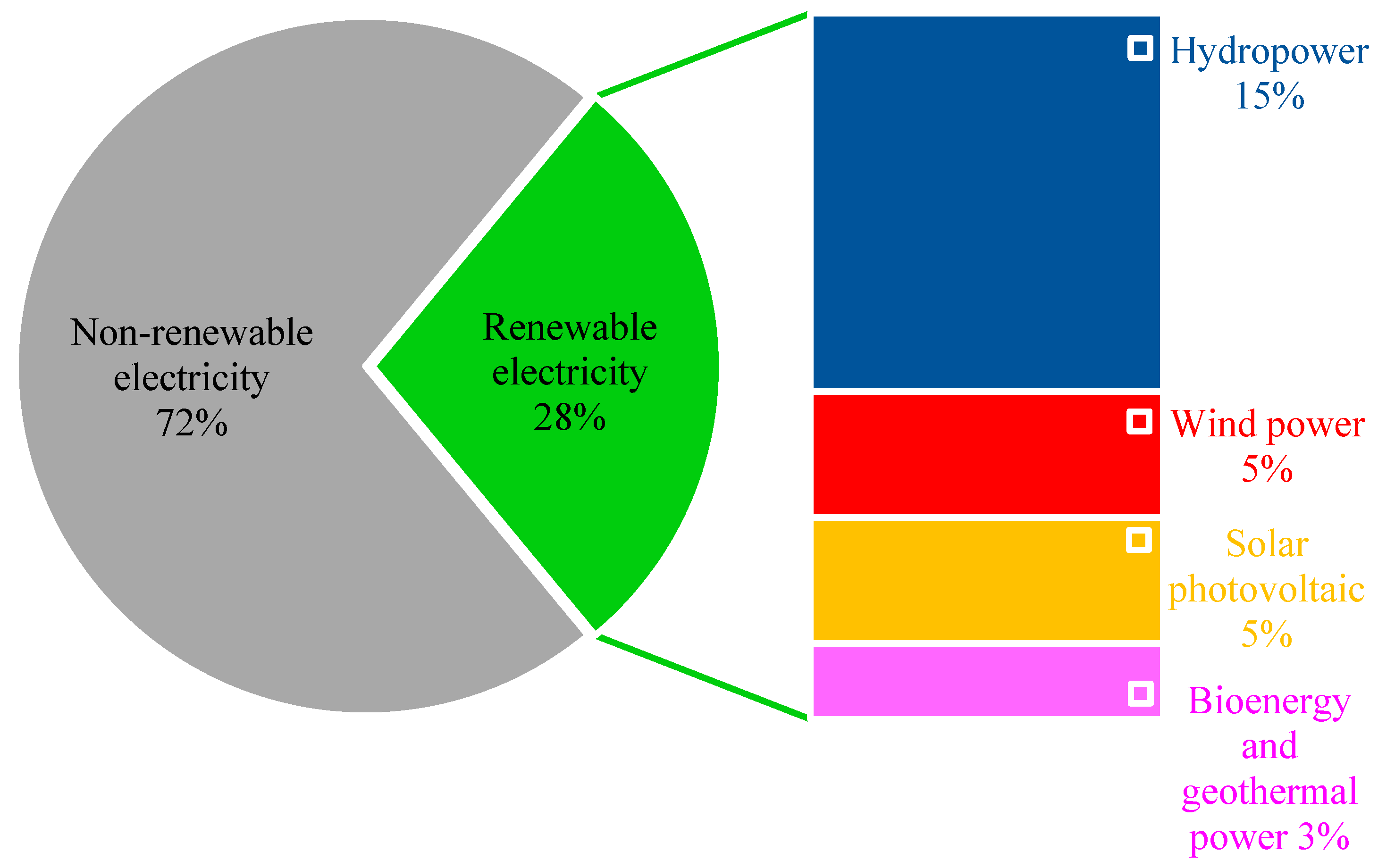
Figure 1. Worldwide wind power share of global electricity production in 2021 [4].
Electronics 12 01597 g001
Figure 2. The topology of a wind turbine system.
Electronics 12 01597 g002
Figure 3. The block diagrams of EMD algorithm and EEMD algorithm. (a) EMD; (b) EEMD.
Electronics 12 01597 g003
Figure 4. Simulation model of the converter.
Electronics 12 01597 g004
Figure 5. Simulated line-to-line voltage Uabcg (Uab, Ubc, Uca). (a) Normal state; (b) OC fault in T1.
Electronics 12 01597 g005
Figure 6. Permutation entropy of 22 fault modes of the converter. (a) m = 3; (b) m = 9.
Electronics 12 01597 g006aElectronics 12 01597 g006b
Figure 7. Effects of m on diagnostic results. (a) Accuracy; (b) Time-consuming.
Electronics 12 01597 g007
Figure 8. Comparation of different methods to highlight EEMD. (a) Comparation of average diagnostic accuracy; (b) Comparation of calculation time.
Electronics 12 01597 g008
Figure 9. Comparation of different methods to highlight PE. (a) Comparation of average diagnostic accuracy; (b) Comparation of calculation time.
Electronics 12 01597 g009
Table 1. The steps of EMD algorithm.
StepsEMD Decomposition
Step 1Initialization: r 0 = x ( t ) , i = 1
Step 2Calculate the i th oscillation mode I M F i
Step 2 (a)Set c i ( q 1 ) ( t ) = r i 1 ( t ) , q = 1
Step 2 (b)Calculate the local extremum of c i ( q 1 ) ( t )
Step 2 (c)Use cubic spline to interpolate the local extremum to obtain the lower envelope e min ( t ) and upper envelope e max ( t )
Step 2 (d)Average the lower and upper envelopes: ψ i ( q 1 ) ( t ) = ( e max ( t ) + e min ( t ) ) / 2
Step 2 (e)Calculate the detailed component: c i q ( t ) = c i ( q 1 ) ( t ) ψ i ( q 1 ) ( t ) . If c i q ( t ) satisfies IMF conditions, then set d i ( t ) = c i q ( t ) , that is I M F i ; else go to step 2 (b) and q = q + 1
Step 3Obtain residue: r i + 1 ( t ) = r i ( t ) d i ( t ) . If r i + 1 ( t ) has more than one extreme, then go to Step 2 and i = i + 1 ; else the procedure is ended and r i + 1 ( t ) is residue
Table 2. The steps of EEMD algorithm.
StepsEEMD Decomposition
Step 1Add white noise to the original signal to obtain a new signal: x δ ( t ) = x ( t ) + w δ ( t ) ,   δ = 1 , 2 , , ρ , where ρ is the number of ensemble realizations, w δ ( t ) is the δ th independent white noise
Step 2 Decompose   x δ ( t ) by EMD and obtain a group of IMFs: d i , δ ,   i = 1 , 2 , , I , where I is the number of IMFs, d i , δ is the i th IMF of the δ th realization
Step 3Average all realizations to obtain final I M F ¯ :   d i ¯ = 1 ρ δ = 1 ρ d i , δ , where i = 1 , 2 , , I and δ = 1 , 2 , , ρ
Table 3. Main parameters of the simulated converter model.
QuantityValueQuantityValue
Rated voltage575 VStator leak inductance0.18 pu
Rated power1.5 MWRotor leak inductance0.16 pu
Pole pairs number3Stator resistance0.023 pu
Magnetizing inductance2.9 puRotor resistance0.016 pu
Table 4. The diagnosis results of 22 faults.
Fault ModeAccuracy (%)
m = 3m = 4m = 5m = 6m = 7m = 8m = 9
Normal96.8750100100100100100100
T190.625090.625093.750010093.750096.875096.8750
T210010010096.8750100100100
T390.625090.625010093.750096.875096.8750100
T481.250084.375090.625093.750093.750096.875096.8750
T593.750093.7500100100100100100
T610090.625010010096.8750100100
T1T2100100100100100100100
T3T4100100100100100100100
T5T696.875096.8750100100100100100
T1T387.500090.625087.500096.875010010093.7500
T1T596.875084.375096.875010010096.8750100
T3T593.750010090.625010096.875096.875096.8750
T2T493.750096.875010096.875010096.8750100
T2T696.875096.875010096.875096.875096.875096.8750
T4T696.8750100100100100100100
T1T410010010096.875010096.8750100
T1T693.750010010096.875096.8750100100
T3T271.875090.625093.750010096.875093.750096.8750
T3T610010010096.8750100100100
T5T293.750010010096.875096.875010096.8750
T5T493.750096.8750100100100100100
Average94.034195.596697.869398.295598.437598.579598.8636
Standard deviation6.81315.25213.90392.09682.10191.86191.8159
Table 5. The diagnostic results of the proposed method for all noise conditions.
Noise
Conditions
StabilityEvaluation Indicators (%)
AccuracyPrecisionRecallF1-ScoreSpecificityFARMAR
20 dBMinimum96.875096.975896.875096.865499.85120.05411.1364
Maximum98.863698.896598.863698.862999.94590.14883.1250
Average97.822097.910897.822097.818699.89630.10372.1780
Standard deviation0.57350.53870.57350.57560.02730.02730.5735
15 dBMinimum94.318294.515594.318294.308599.72940.09471.9886
Maximum98.011498.080698.011498.008699.90530.27065.6818
Average96.302196.438796.302196.293999.82390.17613.6979
Standard deviation0.86160.83810.86160.86600.04100.04100.8616
10 dBMinimum85.795586.257385.795585.810599.32360.45329.5170
Maximum90.483090.707490.483090.465899.54680.676414.2045
Average88.120388.507388.120388.092499.43430.565711.8797
Standard deviation1.03541.03191.03541.03200.04930.04931.0354
5 dBMinimum72.301172.603072.301172.274198.68101.001121.0227
Maximum78.977379.592978.977378.960598.99891.319027.6989
Average75.937576.446775.937575.855398.85421.145824.0625
Standard deviation1.67641.74111.67641.66510.07980.07981.6764
Table 6. Comparison with previous schemes.
SchemeFault TypesTraining to Testing RatioNumber of RunsNoise
Conditions
Average
Accuracy (%)
Standard Deviation of Accuracy (%)
EEMD-PE22 OC faults3:23020 dB97.82200.5735
15 dB96.30210.8616
10 dB88.12031.0354
5 dB75.93751.6764
MEMD-FE [12]22 OC faults3:23030 dB95.57581.9344
20 dB92.14771.3312
10 dB84.23381.7167
EEMD-NE [11]22 OC faults3:23020 dB99.2756-
15 dB97.8598-
10 dB90.0758-
5 dB71.8040-
Disclaimer/Publisher’s Note: The statements, opinions and data contained in all publications are solely those of the individual author(s) and contributor(s) and not of MDPI and/or the editor(s). MDPI and/or the editor(s) disclaim responsibility for any injury to people or property resulting from any ideas, methods, instructions or products referred to in the content.