Abstract
The operation cost waste in the charge and discharge process cannot be ignored for islanded microgrids with energy storage units. Different from the economic dispatch methods focused on the power pricing and bid coefficient in the tertiary control layer, this paper designed a power management algorithm for the economic operation of energy storage units in the secondary control layer. The strategy is devoted to minimizing the total charge power cost of energy storage units while satisfying the constraint of power balance. Meanwhile, the maximized allowable delay bounds were derived to guarantee the communication network reliability when against random time delays. The system stability was analyzed by the Lyapunov functions. Finally, the numerical simulations on the modified IEEE 30 feeder model verify the superiority of the provided algorithm.
1. Introduction
Unlike AC microgrids influenced by reactive power regulation and frequency fluctuations, DC microgrids are easier to control and attract academic interest. The hierarchical structure is a conventional method used to control islanded DC microgrids. Based on different time scales, the hierarchical structure can be operated with separated control layers, including primary, secondary, and tertiary control layers [1,2]. In the primary control layer, the voltage-based droop curve can adjust the active power output to maintain voltage stability after disturbance and generate steady-state voltage deviation. In the secondary control layer, voltage deviation can be eliminated with the distributed controller. In the tertiary control layer with the longest time-scale, the output of the power system can be dispatched in the economical operation [3,4,5].
Most previous studies focused on power scheduling to realize economic dispatch at the tertiary control layer. Specifically, multiple kinds of neural network algorithms have been applied in the tertiary control layer to regulate power allocation for economic dispatch. In [6], an improved hybrid bat method is proposed to achieve balanced power distribution. This method considers the reactive power dispatch and optimizes the combined scheme. Ref. [7] proposed a squirrel search method to address the environmental and economic active power sharing issue by ensuring the diversity of Pareto-optimal solutions. Some extreme scenarios were considered in [8] to guarantee the day-ahead economic dispatch of islanded microgrids with wind power. Based on a quadratic programming method, the proposed economic dispatch could solve wind power limitation and load-shedding problems. In order to address the economic dispatch issue with different scenarios, ref. [9] combined the Lagrangian relaxation method and the proximal method for faster convergence. Moreover, power pricing is an essential factor in addressing the economic dispatch issue of multi-microgrid systems. To realize power dispatch following demand forecasts, a temporal locational marginal pricing method is provided in [10]. However, neural network algorithms, scenario-based solutions, and pricing strategies focused on the day-ahead power dispatch at the tertiary control layer but ignored the economic dispatch at the secondary control layer.
In the secondary control layer, the economic dispatching issue can be divided into two aspects: the generation cost minimization of the generator unit and the charging/discharging power cost minimization of the energy storage unit. For generator units, ref. [11] presented an automatic generation control method to establish the necessary and sufficient conditions for maintaining the global minimum of steady-state synchronous generator outputs. Considering the constraints of local generators, ref. [12] designed a distributed optimization method to achieve the optimal method of the economic dispatch issue. Ref. [13] addressed the network-overloading problem using particle swarm optimization. In particular, the excessive loads could be balanced with the operating generators. Local constraints could be satisfied, and the load could be dispatched to each distributed generation (DG) using a decentralized optimization method with a penalty function in [14]. Compared with power generation units, there are few research studies on the economic dispatch of energy storage units. By employing a mixed-integer linear programming strategy, ref. [15] calculated the lowest levelized cost of energy storage units (ESUs) and evaluated the generation cost, hence determining the Pareto optimal storage configuration. Considering the microgrids with multisource, ref. [16] designed a multi-objective optimal method to achieve a profitable comprehensive income and eliminate factors that cause system instability. In order to expand the economic application of energy storage units, this paper cares about the solutions used to minimize the operation cost of batteries during the charging/discharging process.
The communication network plays a key role in the control process at the secondary control layer. In order to maintain the robustness of communication links, ref. [17] presented a consensus-based distributed method used to realize the optimal dispatch of active power. Meanwhile, the delay bound was calculated by the generalized Nyquist criterion in [17]. Ref. [18] focused on the coexistence delay of the communicate process and transmit process and provided a novel combined-delay-based augmented Lyapunov functional to describe the sampling pattern. Based on the linear matrix inequalities, the system stability could be guaranteed. By employing an aperiodic communication method, ref. [19] relaxed the periodicity of the intermittent data transmission and saved the communication resource. Furthermore, the possibility of time delay is not fixed in the communication network. Hence, the influence of random delay cannot be ignored. To solve the random communication delay problem, ref. [20] proposed a random delay model with conditional probabilities and provided a novel state estimator with a random parameter matrix Kalman filter. To satisfy the constraint of supply/demand power, ref. [21] calculated the maximized allowable bound to maintain the system stability with an economical operation. However, the impact of random delay on the information transmit process of ESUs has received little attention.
Summarizing the above analysis, the current distributed economic power dispatch method did not address the operating waste issue of energy storage units in the secondary control layer well. Meanwhile, the power balance constraint of batteries should be considered in the control process. To maintain the communication network stability in the secondary control layer, it is essential to further research how to deal with randomly occurring time delays in communication links.
In order to address the above shortcomings, this paper presents a distributed cooperative economic dispatch algorithm for energy storage units. The salient novel contributions of this paper are:
1. Different to economic dispatch methods for generator units, we provided a distributed cooperative method to minimize the total charge power cost of energy storage units. A second-order polynomial function was used to describe the operating cost of batteries, and Lagrange optimization methods were used to coordinate incremental costs.
2. In order to meet the constraint of power balance, we added a power mismatch auxiliary variable to the controller. This variable can adjust the injected/output power of each node and ensure the balance constraint during the control process.
3. To work against the random time delay in the communication network, we derived the maximum allowable boundary of delay based on the probability of delay occurrence. The closed-loop system stability analysis and simulation show the robustness of the presented solution.
This paper is organized as follows. Preliminaries are provided in Section 2. An economic distributed algorithm for energy storage units with random time delay is developed in Section 3. In Section 4, different cases are proposed to verify illustrative results. Finally, Section 5 concludes the paper.
2. Preliminaries
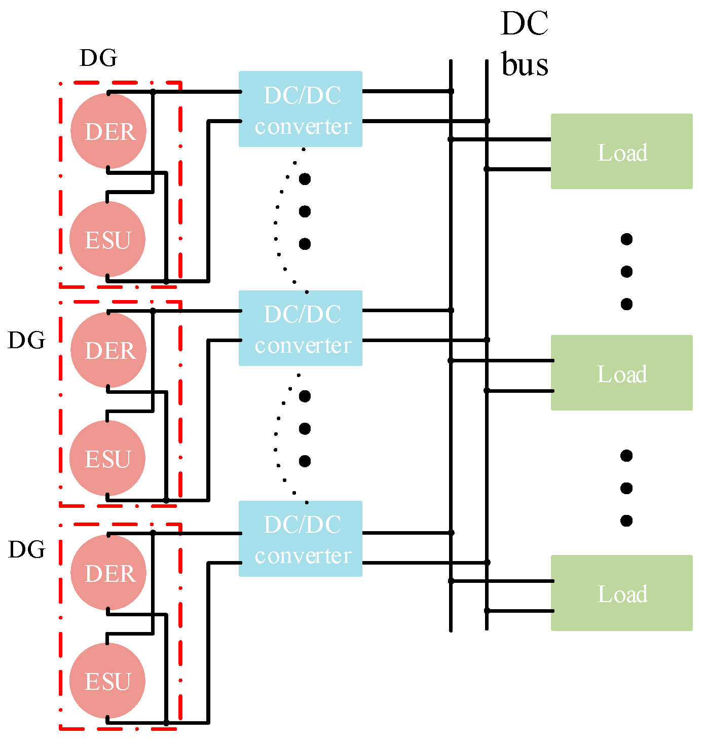
The islanded DC microgrid consists of a physical network and communication network. The physical network is composed of six DG nodes, as shown in the red box in Figure 1. Each DG is connected to the DC bus by the corresponding DCDC converter, which contains the local primary controller and the distributed secondary controller. Through the local primary controller, each node can eliminate voltage deviation and power fluctuation through droop control. Based on the communication network (black dotted line) in Figure 1, the distributed secondary controller can exchange state information and realize the control objectives.
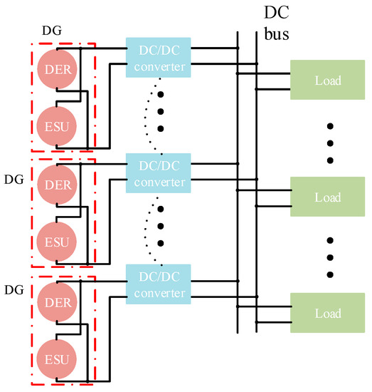
Figure 1.
The islanded DC microgrid structure.
2.1. Algebraic Graph Theory
Complex network system G(N,E) can describe the islanded DC power system with an energy storage unit. N is the node set, and each DG node contains a PV unit and a battery unit. Edge set E is E ∈ N × N. Moreover, the communication network for the complex network system can be described as adjacency matrix A = [aij] and Laplace matrix L = [lij], where aij describes the coupling relationship between node i and j, and lii = ∑i≠j aij, lij = −aij. Note that the Laplace matrix satisfies ∑lij = 0. The nominal value is given by the virtual leader, while gain matrix B = diag{g1, …, gN} represents the communication links with the virtual leader node. Specifically, V* is set as the nominal voltage, and the total load PL is a constant.
2.2. Economic Dispatch
In order to realize the economic operation of energy storage units, the total operation cost of batteries should be minimized; hence, the optimization problem can be defined as:
The control objective in (1) is to minimize the total charge cost and battery consumption power. The charge efficiency defines the actual charge power and charge power, which can be described as νi = −αiPB,i + βi. Inspired by [22], the charge efficiency function is a fitted polynomial curve, where αi is the first-order fitting parameter, and βi is the constant fitting parameter. Moreover, the power balance constraint should be satisfied with the total generation power ∑PG,i and the total load demand ∑PL,i. Then, the increment cost variable is used to solve the optimization problem by the Lagrange function .
2.3. Control Structure
In the islanded DC power system, the node voltage and active power output are the most important control objectives. Based on the voltage droop control rule [23], the voltage Vi changes with active power output Pi in the ith converter through
where Pi*, Di, and V* are the nominal power, droop parameter, and nominal voltage, respectively. It can be seen that, once the local load PL,i fluctuates with ∆PL,i, the voltage deviation becomes nonzero. The secondary controller in the DC/DC converter then adjusts Pi* for the power compensation ∆PL,i. Consider the injected/output power balance. There exists Pi = PG,i − PB,i in each node, where PG,i and PB,i are the power generation and the charging power for the battery unit, respectively. Hence, to force for all agents, the secondary controller forces the nominal power to track the reference Pi* = P*i,ref = PG,i − PB,iref. The control objective of the primary droop controller and the secondary controller can be defined as:
3. Proposed Control Scheme
Inspired by [21,22], this paper constructed an islanded power system that consists of a physical power system and communication network. The physical power system is composed of multiple distributed generation (DG) nodes, each containing a renewable energy source (RES) generation unit and an energy storage unit. Meanwhile, the communication links between the DC/DC converters constitute the communication network. In order to reduce the charging power loss in the physical power network and avoid the random delay in the communication system, we provided a distributed cooperative control algorithm for the economic operation of a battery with random delay effects.
3.1. Distributed Cooperative Control for Economic Operation
3.1.1. Voltage Restoration
To eliminate voltage deviations and force voltages to follow the reference values, we propose a leader–follower control method as follows:
When the node can connect to the virtual leader node, the connection parameter gi ≠ 0; otherwise, gi = 0. Considering all nodes, Equation (4) can be combined into matrix form , where G is the communication connection matrix.
3.1.2. Power Balance
The operation cost of the power system can be minimized when increment costs of different batteries are controlled to be synergized. Hence, a distributed consensus algorithm with second-order dynamics was designed to realize the control objective. Meanwhile, the auxiliary power mismatch variable ρi was added into the control process to meet the constraint of power balance:
Based on the relationship between PB,i and , we can obtain the corresponding charging power when incremental costs are consistent. Furthermore, the power mismatch variable ρi ensures the balance of injected/released power in the control process.
Similarly, Formula (5) can be expressed as matrix form (6) when combining all nodes:
Through Formulas (4) and (5), we can achieve the control objectives of voltage restoration and economic dispatch while maintaining power balance, which is shown as:
Continuous information exchange is necessary for realizing the control objectives, so it is essential to ensure communication reliability. To avoid the effect of random delay on the control process, we contributed to proposing practical constraints.
3.2. Distributed Cooperative Control for Economic Dispatch with Random Delay Effect
The states of converters are transmitted via the communication network, which is formed as the data packet. Each local controller updates its own state when receiving the latest data packet. Consider the randomly occurring packet dropouts. The variables ε(t) are proposed to describe the transmission status. ε(t) are independent Bernoulli-distributed white sequences with
where ε’ ∈ [0, 1] is defined as the random dropout rates in the communication process.
Subject to random packet loss, the control input should be modified with the probabilistic random variable ε(t) in the signal transmission:
Obviously, economic dispatch variable and power imbalance variable ρ are applied in Equation (9) to design the control input. Suppose that different variables communicate with various information channels. It will be easier for the stabilization of systems to become broken. Therefore, we transformed Equation (9) into the matrix form, which aims to package these two variables into a single packet to reduce the risk of communication.
For the sake of simplicity, we converted Equation (10) to:
where , , .
In the communication network of the closed-loop power system, each agent has an information sender and receiver. The sender can package its own status information to neighbors, as shown by the blue line, whereas the receiver can obtain the status information of neighbors, as shown by the green line. It is evident that the data transmission process is interfered with by random delay, whose occurrence probability is ε’.
Note that the random time delays in communication links can be constructed as stochastic variable functions satisfying the Bernoulli-distributed white sequence.
Definition 1.
The model (11) is exponentially mean-square stable by the positive constants b1 and b2, so there is , where can represent in this paper.
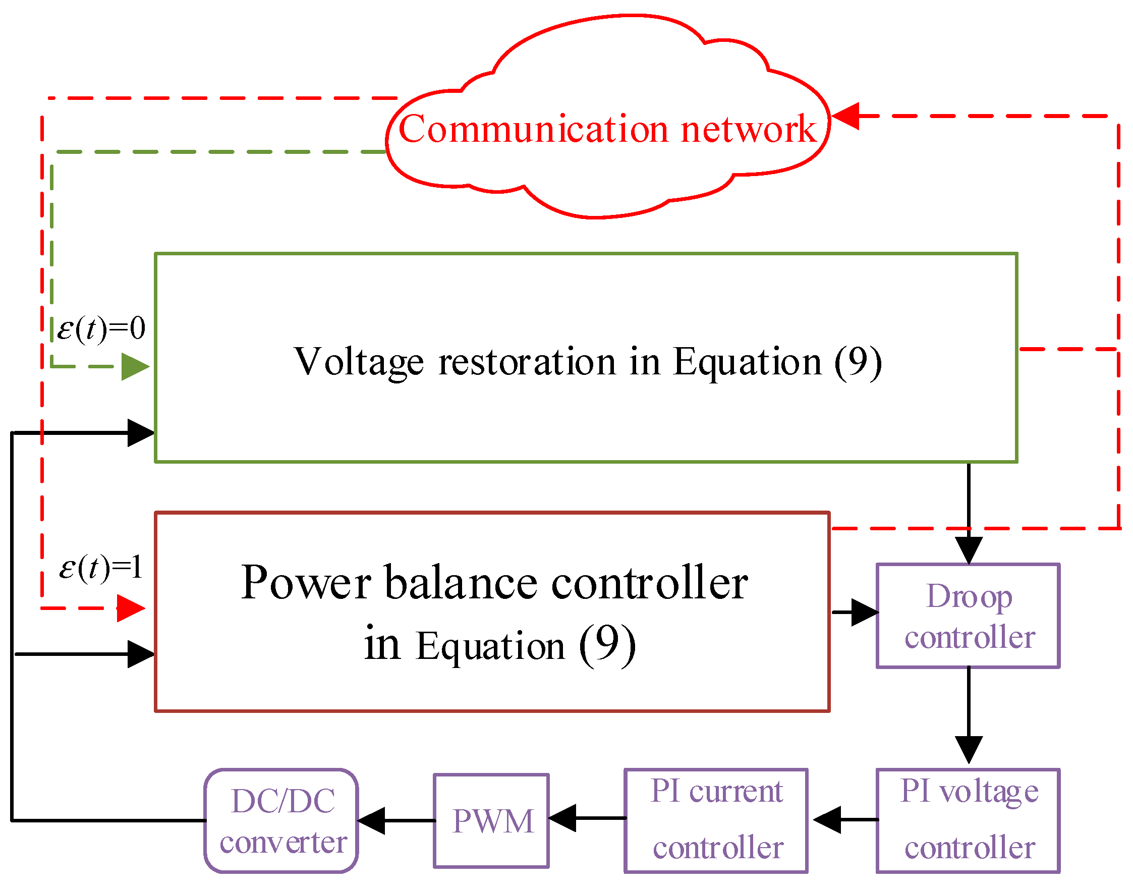
Based on Equations (2) and (9), a primary/secondary control framework can be designed to realize the control objectives (7), which is shown in Figure 2. In the secondary control layer, each agent exchanges state information with its neighbors in the communication network. Some information packets can be transmitted successfully, which are marked by red lines. Furthermore, the other information packets are affected by random delays, which are marked by green lines. Then, the secondary controller on each converter calculates the corresponding reference voltage and the reference charging power through the collected state data affected and not affected by the delay and sends the corresponding reference value to the primary controller. The primary controller then calculates the deviation between the actual voltage and the reference voltage and the deviation between the actual charging power and the reference charging power, and finally adjusts the output of the DC/DC converter through the PWM wave.
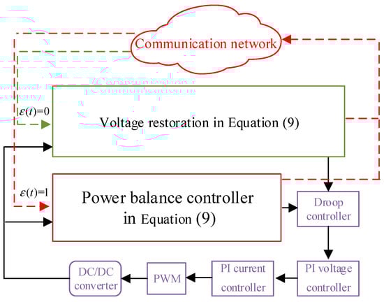
Figure 2.
Distributed cooperative control framework.
3.3. Stability Analysis
3.3.1. Voltage Restoration
Inspired by [21], the error system should be defined to ensure the stability of the voltage restoration process, where . Hence:
where LV is the Laplace matrix and GV is the gain matrix.
Theorem 1.
Given communication parameter , the close-loop system (12) has exponential mean-square stability if there exists a delay bound for the communication delay τV. Then, the voltage can be forced to the reference in the control process.
Proof of Theorem 1.
Consider the Lyapunov function candidate:
Hence, we have:
In , the last term follows:
Note that ε(t) (1 − ε(t)) = 0:
Then, it can be obtained that:
where
By , we have:
where
In order to satisfy , there exist the following inequalities:
which can be expressed by:
Therefore, the allowable bound of delays are:
. □
3.3.2. Economic Power Sharing
In order to guarantee economic power sharing among energy storage units, the stability of the communication network must be verified. Error vector is applied to prove the system stability, where
In addition, the error system of the controller can be described as:
Theorem 2.
Given communication parameter , the close-loop system (25) has exponential mean-square stability if there exists a delay bound . Then, the incremental cost can be synergized, and the economic power sharing can be realized with the power balance constraint.
Proof of Theorem 2.
Construct a Lyapunov functional as:
By using the time derivative of (26), we can obtain:
Note that follows the inequality:
Then,
It can be shown that:
where
Apply mathematical expectations of , such that:
where
Then, we can obtain the allowable delay bound:
In addition, the upper bound of τB can be expressed as:
. □
Remark 1.
Note that there are two allowable delay upper bounds τVmax and τBmax in the process of voltage recovery control and SOC balance economy control, respectively. Therefore, the upper limit of the allowable delay of the entire system should take the minimum value between the two; that is, τmax = min{τVmax, τBmax}.
4. Simulation
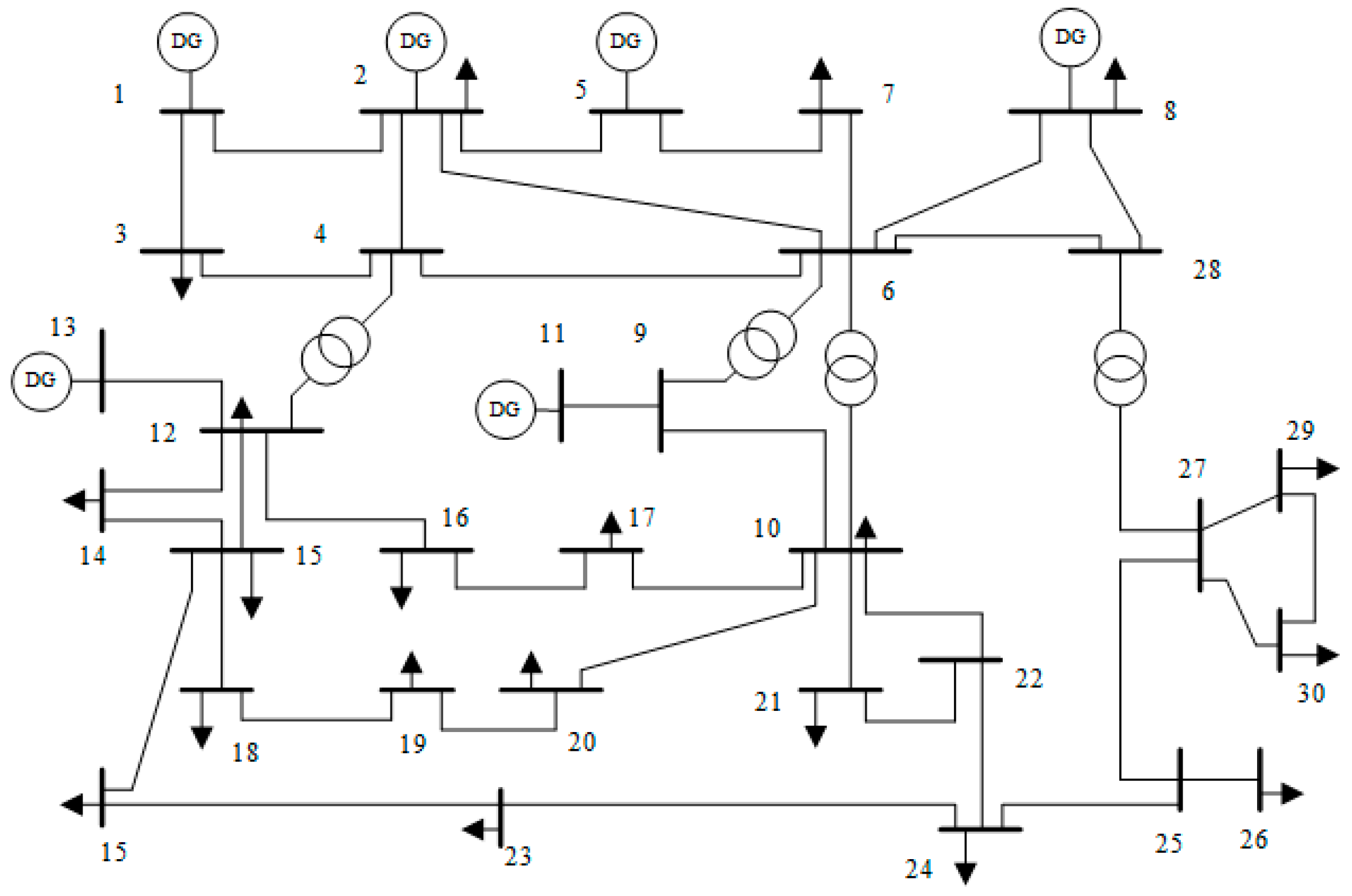
By employing an islanded microgrid modified from the IEEE 30 bus test system, the algorithm validity and model rationality can be verified when against random communication delay. The system includes 6 DGs, 4 transformers, and 37 lines. A 50 kWh battery was chosen as the energy storage unit in DG node. Each node has a 0.6 kΩ local load, and the line impedances are converted into the local load. Moreover, a 0.4 kW load connected to node 7 can be cut out or reconnected by the breaker, which is shown in Figure 3. The control coefficient, electrical coefficient, and reference value are shown in Table 1. By employing the stability analysis, the maximum delay boundary of the voltage recovery control algorithm is 0.22 s, whereas that of the economic control algorithm is 0.18 s. The whole system can be stable when the delay range is 0–0.16 s.
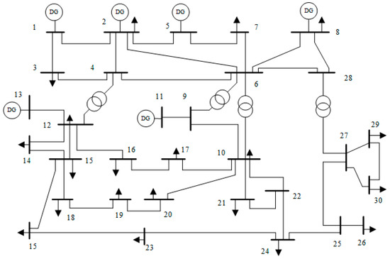
Figure 3.
IEEE30 feeder model (The numbers 1–30 indicate the position of the bus).

Table 1.
Coefficients and related parameters of the power system.
4.1. Case 1: Normal Operation
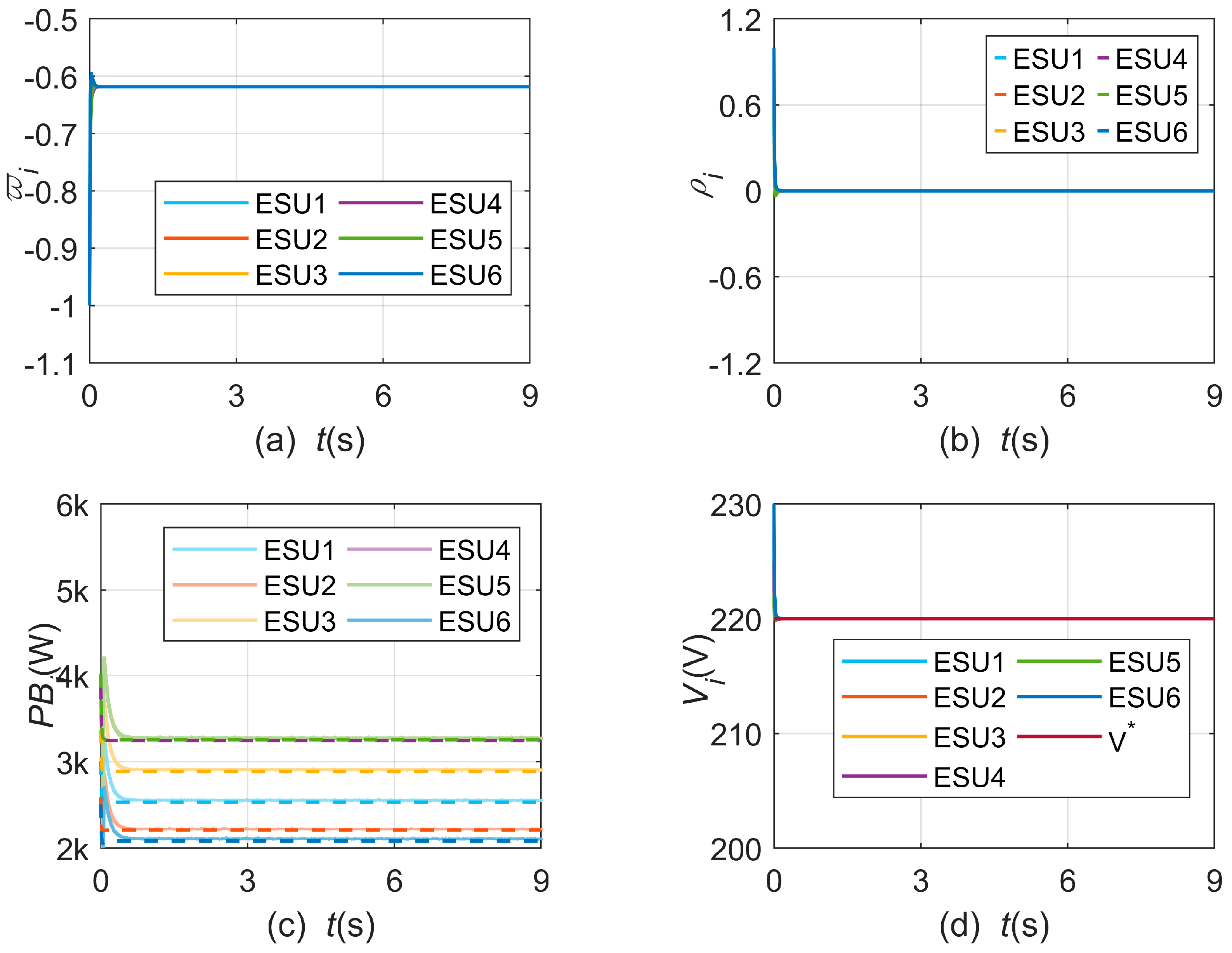
The real-time simulation results with random communication delay are demonstrated in Figure 4. In the control period t = 0–4 s, the increment cost of different agents can be synergized to −0.62 with the impact of random delay. The power mismatch variable can be forced to zero in the control process, which means that the power mismatch between different agents is eliminated with the distributed secondary controllers. Based on the increment cost variables and power mismatch variables, the references of charge power are calculated in the corresponding converters. Then, the actual charge power can follow the reference with the primary controllers. Hence, the total operation cost can be minimized with the power balance constraint, and the voltages can be controlled to the nominal values.
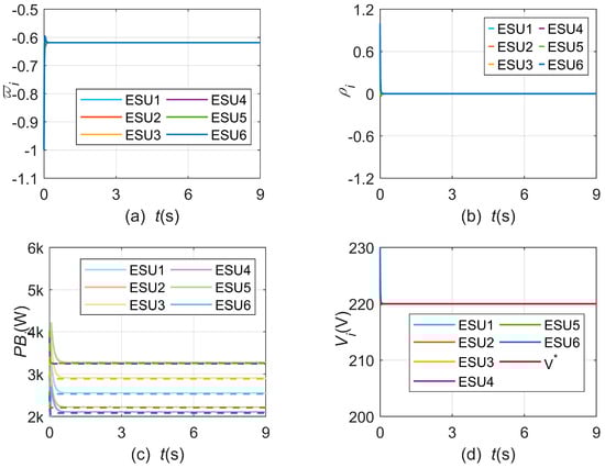
Figure 4.
Normal operation: (a) incremental cost variable; (b) power imbalance variable; (c) charging power (the reference is represented by the dotted line and the actual value represented by the solid line); (d) voltage.
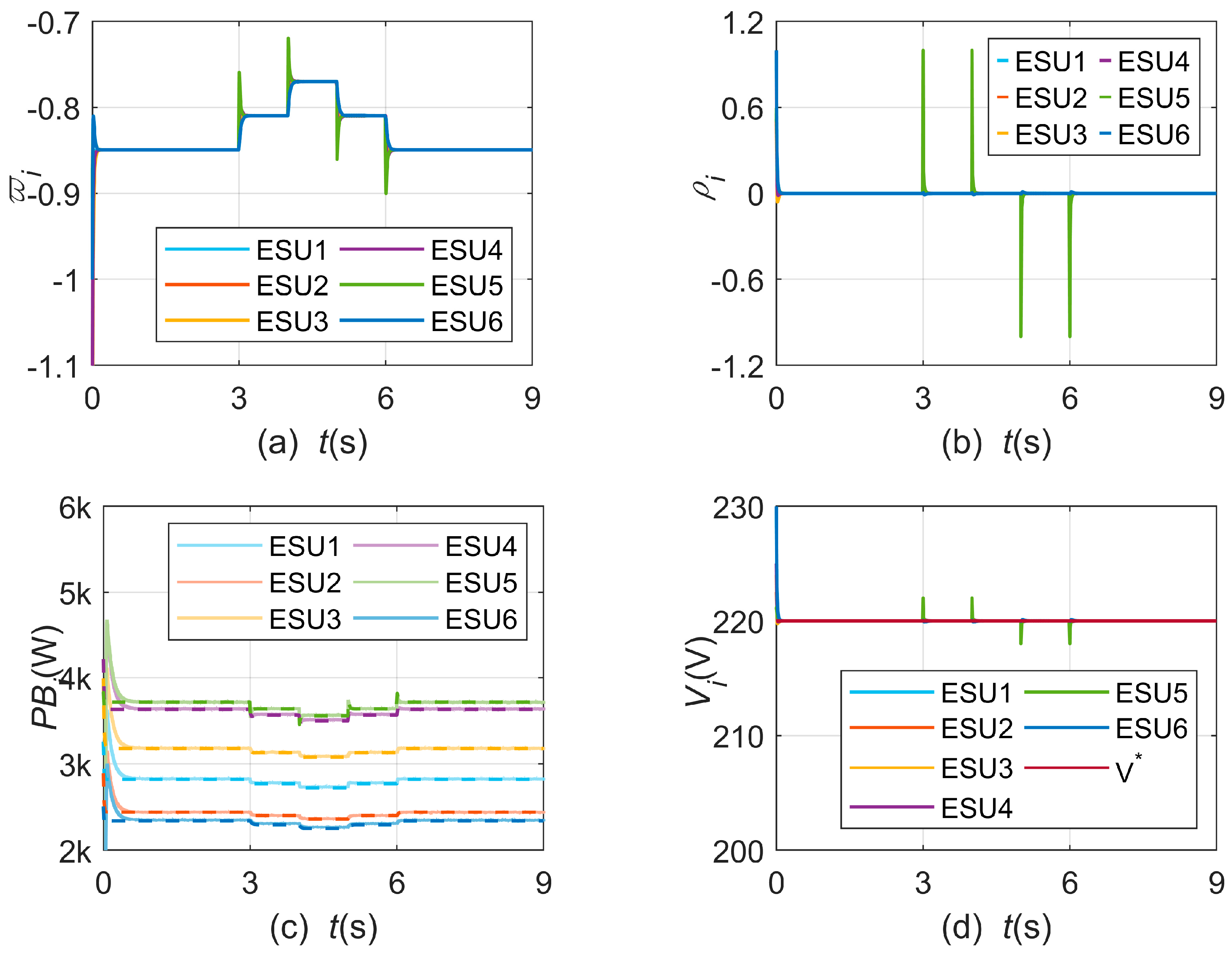
4.2. Case 2: Load Variation
The effectiveness of the presented algorithm in the situation of random delay and load fluctuation is verified in this subsection.Between t = 3 s and t = 6 s, the added load connects to the DG5. Moreover, an extra 0.5 kW load is added in DG4 at t = 4 s and disconnected at t = 5 s. It can be seen that, with the connection and disconnection of the load, the power mismatch variable ρ will produce large fluctuations, thus destroying the stability of the incremental cost variable. However, the designed controller can re-calculate the corresponding charging power reference value according to the balance constraint in a relatively short time. With the actual charging power following the above reference value, the system can be restored to stability, and the voltage fluctuation caused by load variations can be eliminated, as shown in Figure 5.
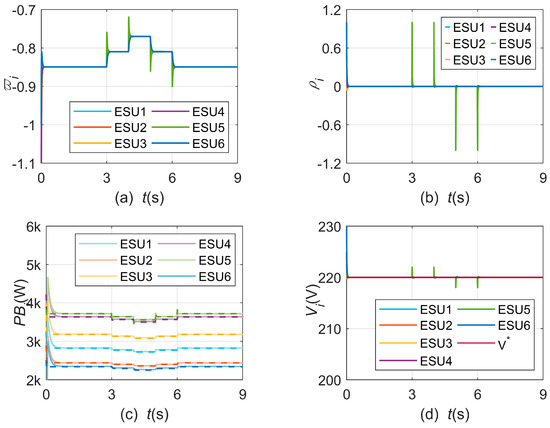
Figure 5.
Load variation: (a) incremental cost variable; (b) power imbalance variable; (c) charging power; (d) voltage.
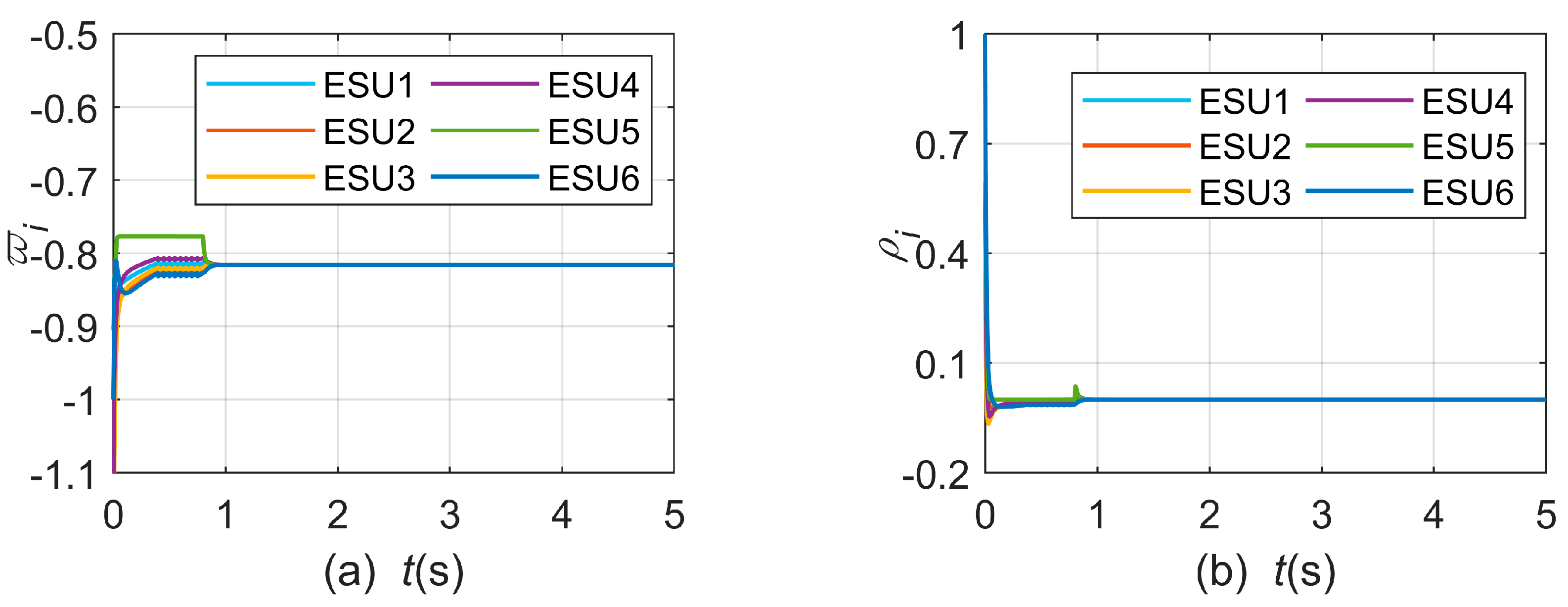
4.3. Case 3: Communication Failure
The stability of communication links plays a vital role in the control process. In order to verify the robustness of the designed communication model, case 3 simulates a single point fault that occurs on the communication link between DG4 and DG1 at t = 0.1 s and t = 4 s, respectively, and disappears at t = 0.8 s and t = 4.5 s. When t = 0.1 s, the synchronization rates of the incremental cost variable , the power imbalance variable ρ4, and the voltage V4 in DG4 are significantly lower than those of the normal operation. However, these three variables can still quickly enter the cooperative state when the communication link is restored at t = 0.8 s. After t = 4 s, the system enters a stable state; hence, the single point fault on the communication link has little impact on the system. The incremental cost variable, power mismatch variable, and voltage maintain stability with communication failure, as shown in Figure 6.
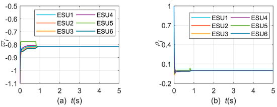
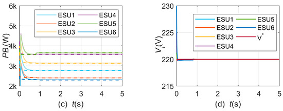
Figure 6.
Communication failure: (a) incremental cost variable; (b) power imbalance variable; (c) charging power; (d) voltage.
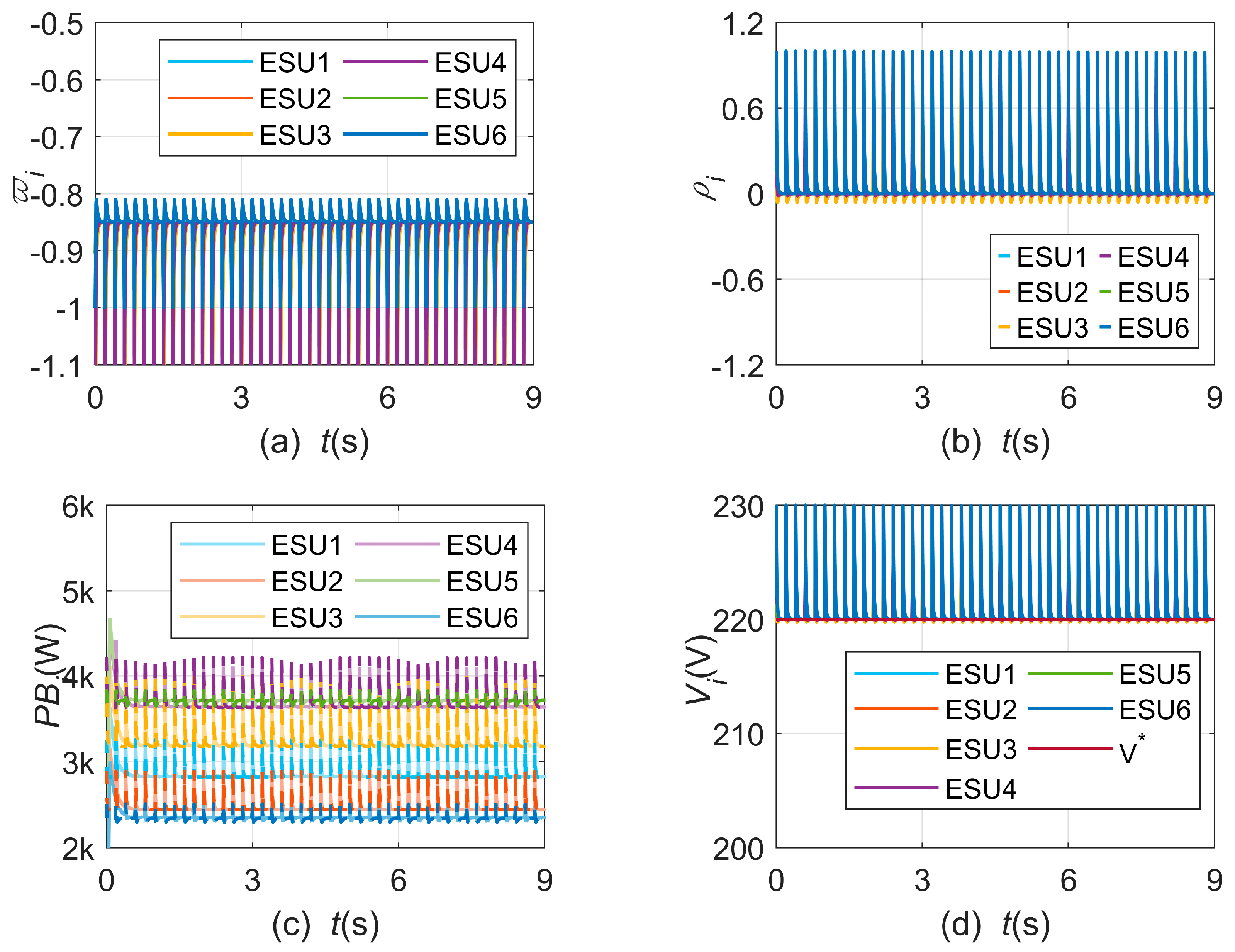
4.4. Case 4: Comparison
Moreover, the effectiveness of the presented algorithm against random communication delay can be verified by comparing it with the traditional distributed secondary control algorithm. Due to data loss and information errors when receiving neighbor information, each agent generates an incorrect reference value when updating its own state. Therefore, the traditional secondary control algorithm produces drastic fluctuations, and the whole system cannot be synergized. The stability of the network is destroyed, and the voltage and charging power cannot track the reference value, which is shown in Figure 7.
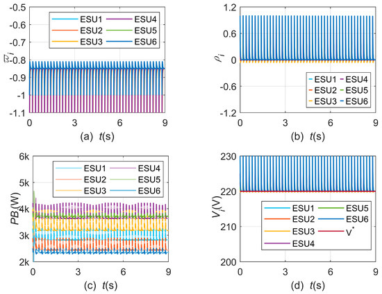
Figure 7.
Comparison: (a) incremental cost variable; (b) power imbalance variable; (c) charging power; (d) voltage.
5. Conclusions
In order to realize voltage restoration and economic dispatch with a power balance constraint, a novel distributed cooperative algorithm was proposed in this paper. In order to further work against the random delay in communication links, an independent Bernoulli-distributed white sequence was applied to ensure the system stability. Based on an IEEE 30-node feeder model, the simulation results show the effectiveness and robustness of the proposed algorithm.
Our future work is to expand the application of the presented method, including charge/discharge mode switching, SOC balance, and AC/DC hybrid microgrid development.
Author Contributions
Conceptualization, S.C. and Q.G.; methodology, S.C.; software, S.C.; validation, S.C., Q.G., and J.C.; formal analysis, S.C.; investigation, S.C.; resources, S.C.; data curation, S.C. and L.F.; writing—original draft preparation, S.C.; writing—review and editing, S.C.; visualization, S.C.; supervision, S.C.; project administration, S.C.; funding acquisition, Q.G. All authors have read and agreed to the published version of the manuscript.
Funding
This research was funded by The National Key R&D Program of China 2020YFB0905905, in part by the National Natural Science Foundation of China under Grants No. 62173257.
Data Availability Statement
Not applicable.
Conflicts of Interest
The authors declare no conflict of interest.
References
- Lai, J.; Lu, X.; Yu, X.; Monti, A. Stochastic Distributed Secondary Control for AC Microgrids via Event-Triggered Communication. IEEE Trans. Smart Grid 2019, 11, 2746–2759. [Google Scholar] [CrossRef]
- Lai, J.; Lu, X.; Yu, X.; Yao, W.; Wen, J.; Cheng, S. Distributed Multi-DER Cooperative Control for Master-Slave-Organized Microgrid Networks with Limited Communication Bandwidth. IEEE Trans. Ind. Inform. 2018, 15, 3443–3456. [Google Scholar] [CrossRef]
- Hosseinzadeh, M.; Schenato, L.; Garone, E. A distributed optimal power management system for microgrids with plug&play capabilities. Adv. Control. Appl. 2021, 3, 65. [Google Scholar]
- Liu, G.; Ferrari, M.F.; Ollis, T.B.; Tomsovic, K. An MILP-Based Distributed Energy Management for Coordination of Networked Microgrids. Energies 2022, 15, 6971. [Google Scholar] [CrossRef]
- Alagoz, B.B.; Kaygusuz, A.; Karabiber, A. A user-mode distributed energy management architecture for smart grid applications. Energy 2012, 44, 167–177. [Google Scholar] [CrossRef]
- Liu, J.; Liu, Y.; Liang, H.; Man, Y.; Li, F.; Li, W. Collaborative optimization of dynamic grid dispatch with wind power. Int. J. Electr. Power Energy Syst. 2021, 133, 107196. [Google Scholar] [CrossRef]
- Sakthivel, V.P.; Suman, M.; Sathya, P.D. Combined economic and emission power dispatch problems through multi-objective squirrel search algorithm. Appl. Soft Comput. 2021, 100, 106950. [Google Scholar] [CrossRef]
- Xu, J.; Wang, B.; Sun, Y.; Xu, Q.; Liu, J.; Cao, H.; Jiang, H.; Lei, R.; Shen, M. A day-ahead economic dispatch method considering extreme scenarios based on wind power uncertainty. CSEE J. Power Energy Syst. 2019, 5, 224–233. [Google Scholar] [CrossRef]
- Tang, C.; Xu, J.; Tan, Y.; Sun, Y.; Zhang, B. Lagrangian Relaxation with Incremental Proximal Method for Economic Dispatch with Large Numbers of Wind Power Scenarios. IEEE Trans. Power Syst. 2019, 34, 2685–2695. [Google Scholar] [CrossRef]
- Guo, Y.; Chen, C.; Tong, L. Pricing Multi-Interval Dispatch Under Uncertainty Part I: Dispatch-Following Incentives. IEEE Trans. Power Syst. 2021, 36, 3865–3877. [Google Scholar] [CrossRef]
- Baros, S.; Chen, Y.C.; Dhople, S.V. Examining the Economic Optimality of Automatic Generation Control. IEEE Trans. Power Syst. 2021, 36, 4611–4620. [Google Scholar] [CrossRef]
- Liu, Q.; Le, X.; Li, K. A Distributed Optimization Algorithm Based on Multiagent Network for Economic Dispatch with Region Partitioning. IEEE Trans. Cybern. 2021, 51, 2466–2475. [Google Scholar] [CrossRef] [PubMed]
- Selladurai, R.; Chelladurai, C.; Jayakumar, M. Optimal dispatch of generators based on network constrained to enhance power deliverable using the heuristic approach. Environ. Sci. Pollut. Res. 2022, 22, 1. [Google Scholar] [CrossRef] [PubMed]
- Wang, S.; Xing, J.; Jiang, Z.; Li, J. Decentralized economic dispatch of an isolated distributed generator network. Int. J. Electr. Power Energy Syst. 2019, 105, 297–304. [Google Scholar] [CrossRef]
- Psarros, G.N.; Dratsas, P.A.; Papathanassiou, S.A. A comparison between central- and self-dispatch storage management principles in island systems. Appl. Energy 2021, 298, 117181. [Google Scholar] [CrossRef]
- Hou, H.; Chen, Y.; Liu, P.; Xie, C.; Huang, L.; Zhang, R.; Zhang, Q. Multisource Energy Storage System Optimal Dispatch Among Electricity Hydrogen and Heat Networks from the Energy Storage Operator Prospect. IEEE Trans. Ind. Appl. 2022, 58, 2825–2835. [Google Scholar] [CrossRef]
- Chen, G.; Zhao, Z. Delay Effects on Consensus-Based Distributed Economic Dispatch Algorithm in Microgrid. IEEE Trans. Power Syst. 2018, 33, 602–612. [Google Scholar] [CrossRef]
- Zhang, Y.; He, Y.; Long, F.; Zhang, C.-K. Mixed-Delay-Based Augmented Functional for Sampled-Data Synchronization of Delayed Neural Networks with Communication Delay. IEEE Trans. Neural Netw. Learn. Syst. 2022, 1–10. [Google Scholar] [CrossRef] [PubMed]
- Guo, Y.; Qian, Y.; Wang, P. Leader-following consensus of delayed multi-agent systems with aperiodically intermittent communications. Neurocomputing 2021, 466, 49–57. [Google Scholar] [CrossRef]
- Pang, N.; Luo, Y.; Zhu, Y. A novel model for linear dynamic system with random delays. Automatica 2019, 99, 346–351. [Google Scholar] [CrossRef]
- Yu, M.; Song, C.; Feng, S.; Tan, W. A consensus approach for economic dispatch problem in a microgrid with random delay effects. Int. J. Electr. Power Energy Syst. 2020, 118, 105794. [Google Scholar] [CrossRef]
- Yu, C.; Zhou, H.; Lu, X.; Lai, J. Frequency Synchronization and Power Optimization for Microgrids With Battery Energy Storage Systems. IEEE Trans. Control. Syst. Technol. 2021, 29, 2247–2254. [Google Scholar] [CrossRef]
- Lai, J.; Lu, X.; Monti, A.; De Doncker, R.W. Event-Driven Distributed Active and Reactive Power Dispatch for CCVSI-Based Distributed Generators in AC Microgrids. IEEE Trans. Ind. Appl. 2020, 56, 3125–3136. [Google Scholar] [CrossRef]

Disclaimer/Publisher’s Note: The statements, opinions and data contained in all publications are solely those of the individual author(s) and contributor(s) and not of MDPI and/or the editor(s). MDPI and/or the editor(s) disclaim responsibility for any injury to people or property resulting from any ideas, methods, instructions or products referred to in the content. |
© 2023 by the authors. Licensee MDPI, Basel, Switzerland. This article is an open access article distributed under the terms and conditions of the Creative Commons Attribution (CC BY) license (https://creativecommons.org/licenses/by/4.0/).