A High-Precision Calculation Method for Troposcatter Propagation Delay by Fusing Atmospheric Reanalysis Data

Abstract

Troposcatter propagation delay is one of the most significant sources of errors in troposcatter time comparison. The existing methods of calculating troposcatter propagation delay face problems in terms of effectively reflecting the influence of the meteorological environment on troposcatter propagation delay, due to the insufficient spatial and temporal resolution of the meteorological data. This article proposes a high-precision calculation method for troposcatter propagation delay based on atmospheric reanalysis data. The troposcatter propagation path and the refractive index along the troposcatter data were obtained by combining 3D ray tracing with the European Centre for Medium-Range Weather Forecasts’ Reanalysis 5 (ERA5), with high spatial and temporal resolution. This found the hour-level time delay in troposcatter. The geometric delay, path delay, and total propagation delay of the troposcatter were calculated and analyzed via 12 scattering links in 6 typical geographical regions. It was found that the path delay was the main cause of the propagation delay of troposcatter, and that the proportion of geometric delay in the total propagation delay increased along with an increase in link distance. The propagation delay changed noticeably in different seasons. The path delay was higher in summer and lower in winter, the geometric delay was lower in summer and higher in winter, and the total propagation delay was mainly high in summer and low in winter. There were differences in delay date, seasonal fluctuation amplitude, and in hourly fluctuation standard deviation among different geographic areas.

1. Introduction

Troposcatter communication uses the forward scattering effect from the non-uniform troposphere to propagate radio waves to the area out of sight; this is an important military wireless communication application and has a long single-hop distance, strong obstacle-crossing ability, and good anti-interference and anti-interception performance [1,2]. Troposcatter timing is a method to achieve high-precision time synchronization between distributed stations using troposcatter-channel transmission-time comparison signals. It can overcome limited satellite timing channel resources, short microwave-timing single-hop distances, poor optical fiber timing mobility, and other defects. It is an important supplement to satellite timing, and is a minimum independent timing method in wartime [3]. One-way comparison and two-way comparison are two modes of time comparison based on the scattering channel, whose main source of error is the propagation delay of troposcatter [4].

The propagation delay of troposcatter refers to the difference between the actual propagation time and the ideal propagation time of electromagnetic waves in the tropospheric atmosphere. Electromagnetic waves propagate in the tropospheric atmosphere, and they are affected by the uneven distribution of the atmosphere; their propagation paths are bent, and their propagation velocities change. The actual propagation time is greater than the time taken to propagate along a straight line at the speed of light under ideal conditions. To accurately estimate the propagation delay of troposcatter and to improve the accuracy of time comparison, various delay estimation methods have been proposed. These can be divided into two categories according to different calculation principles:

In the first category, the troposcatter propagation delay is estimated using zenithal delay and mapping function, applying the calculation method of the propagation delay of satellite signals through the troposphere. In [5,6], the method initially obtains surface meteorological data through a meteorological numerical model or from actual measurements. It next obtains the refractive index profile using a refractive index empirical model, then finds the zenith delay through a refractive index integral method, and subsequently combines the zenith delay with the mapping function to obtain the propagation delay. The surface meteorological data in [5] were provided using the GPT2w model, while the surface meteorological data at the station were directly used in [6]. The refractive index profile was obtained using the Hopfield model, and the mapping function uses the CFA2.2 model. This calculation method can be improved. Firstly, the satellite channel passes through the entire troposphere; the propagation delay from the calculation method combines zenithal delay and mapping function through the entire troposphere, while the troposcatter propagates in the troposphere without penetrating the entire troposphere. Secondly, there is a cutoff height angle in satellite channels, and the mapping function principally considers the situation above the cutoff height angle in model fitting. To reduce transmission loss, troposcatter usually utilises a low elevation so as to propagate along the apparent horizontal line of the Earth’s surface; the propagation elevation angle is far smaller than the satellite cutoff height angle.

In the second category, the ray-tracing method was used to calculate propagation delay based on meteorological data. In this method, the propagation path and the refractive index of troposcatter were found by combining meteorological data, the meteorological model, and the meteorological empirical formula with the ray-tracing method, and the propagation delay was obtained by integrating the refractive index along the propagation path. In [7,8,9], the surface meteorological data at the station, the Hopfield model, the UNB3m meteorological model, and the mid-latitude reference atmospheric model were each used to provide meteorological data for the calculation of the ray-tracing method. The ray-tracing method is a high-precision calculation method, and the calculation accuracy of propagation delay is closely related to meteorological data. The meteorological data used in the previously referenced literature were mainly from meteorological numerical models. The empirical values and formulae were obtained through the analysis of a large number of meteorological data, which can reflect the change law of the meteorological environment. To some extent, the numerical meteorological model can reflect the changing conditions in the meteorological environment. However, the meteorological environment is complex and changeable, with a high level of randomness. There is still a great difference between the numerical meteorological model and the actual meteorological conditions.

In recent years, with the continuous improvements in meteorological observation data and the development of data assimilation technology, it has become common to use data assimilation technology to reanalyze meteorological observation data and to reconstruct high-quality, long time series and high-spatiotemporal-resolution historical climate data sets [10,11]. Based on the European Centre for Medium-Range Weather Forecasts (ECMWF), the fifth generation of global atmospheric reanalysis products was already capable of providing meteorological data at a temporal resolution of 1 h and at a spatial resolution of 0.25° × 0.25° [12], which provided the conditions for accurately calculating the propagation delay of troposcatter under different meteorological conditions. For this paper, we constructed a high-precision model to calculate the propagation delay of troposcatter and to analyze the effects of different geographical regions and climatic environments on the propagation delay in six typical regions in China.

2. Propagation Delay of Troposcatter

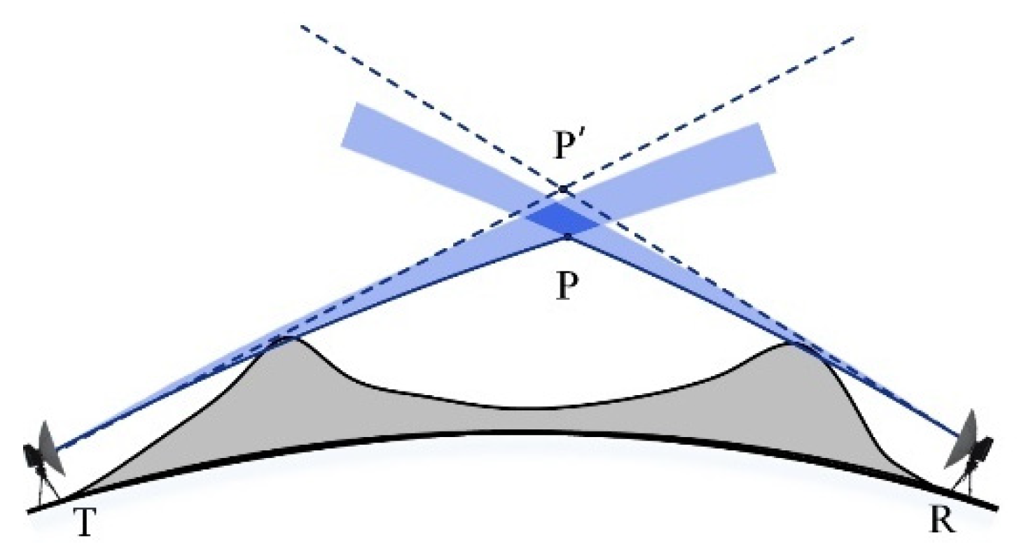
When an electromagnetic wave propagates in the troposphere, in addition to refraction along the way, it is also radiated again by the non-uniform body, and the re-radiation of the radio wave by the nonuniform body in the troposphere is troposcatter [13]. Troposcatter expands the propagation range of electromagnetic waves, enables troposcatter to have the communication ability of over-the-horizon obstacle crossing, overcomes the influence of the curvature of the Earth and obstacles, and spreads the signal to a region hundreds of kilometers away. The propagation principle of troposcatter is shown in Figure 1. T and R are transmitting and receiving antennas, respectively, the dotted line is the central axis direction of the transceiver antenna, and the intersection point P’ of the dotted line is the theoretical scattering point. Affected by the atmospheric refractive index, the beam propagation path bends, and the actual scattering area is lower than the theoretical point. Meanwhile, it is considered that the smaller the antenna elevation angle in the scattering propagation process, the smaller the scattering angle and the lower the transmission loss. Therefore, the path used to calculate the scattering propagation delay is the curve TP and PR close to the apparent plane line in Figure 1. The troposcatter propagation delay is the difference between the time for electromagnetic waves to pass through the curve TP and PR, and the time for electromagnetic waves to pass through the straight line TP’ and P’R under the vacuum condition.

The atmospheric refraction index is defined as the ratio of the propagation speed of an electromagnetic wave in a vacuum to that in a medium

$$n=\frac{c}{v}$$

(1)

In the tropospheric atmosphere, the refraction index is slightly greater than 1, the actual propagation speed of the electromagnetic wave is less than the speed of light, and the actual propagation time from the transmitting end to the receiving end can be calculated by the refractive index integral method

$$t={\displaystyle \underset{\mathrm{TP}+\mathrm{PR}}{\int }\frac{n}{\mathrm{c}}ds}$$

(2)

Then, the propagation delay of troposcatter is

$$\Delta t={\displaystyle \underset{\mathrm{TP}+\mathrm{PR}}{\int }\frac{n}{\mathrm{c}}ds}-\frac{{\mathrm{TP}}^{\prime }+{\mathrm{P}}^{\prime }\mathrm{R}}{\mathrm{c}}$$

(3)

For ease of calculation, the propagation delay is expressed in the form of distance, and it actually contains two parts of delay. One is the length difference between the curved path and the theoretical straight path, which is called geometric delay $\Delta R$. $\Delta R=\Delta t·\mathrm{c}$. The other is the path delay Δr, caused by a change in propagation speed. The propagation delay is the sum of geometric delay and path delay, which reflect the bending and delay effects of atmospheric refractive index on electromagnetic waves, respectively. The solution method is as follows

$$\left\{\begin{array}{l}\Delta g={\displaystyle \underset{\mathrm{TP}+\mathrm{PR}}{\int }ds}-({\mathrm{TP}}^{\prime }+{\mathrm{P}}^{\prime }\mathrm{R})\hfill \\ \Delta r={\displaystyle \underset{\mathrm{TP}+\mathrm{PR}}{\int }(n-1)ds}\hfill \end{array}\right.$$

(4)

3. 3D Ray-Tracing Method

The basis of 3D ray tracing is Fermat’s principle. When the frequency of an electromagnetic wave meets the atmospheric refraction index, it changes in a very small wavelength range, and the ray propagation path can be determined by horse’s principle [14]

$$\delta t=\delta \frac{1}{c}{\displaystyle \underset{S}{\int }nds}=0$$

(5)

where $\delta$ is the variational symbol, $t$ is the propagation time, $c$ is the propagation speed of light in vacuum, $n$ is the atmospheric refraction index, $S$ is the path of light propagation, and $ds$ is the path differential.

To facilitate the calculation of the troposcatter ray propagation path in three-dimensional space, a computational coordinate system is first constructed. The actual Earth is approximately elliptical, and its geometric characteristics are described by the major half-axis, minor half-axis and oblateness of the ellipsoid, and the relationship between the three is

$$f=\frac{a-b}{a}$$

(6)

There are slight differences in the parameters defined in the Earth coordinate system of different protocols. The WGS-84 coordinate system is used in this paper, and the corresponding parameter value is $a=6378137.0 \mathrm{m}$, $b=6356752.3142 \mathrm{m}$ $f=1/298.257223563$ [15].

The communication distance of troposcatter is generally within one thousand kilometers. To reduce the difficulty in calculation, the local sphere is used to replace the Earth’s ellipsoid to construct the calculation coordinate system. The local sphere construction method takes the Earth’s ellipsoid center as the sphere center, and the sphere radius is calculated according to the Euler formula [16] according to the average latitude of the receiver and transmitter

$$\left\{\begin{array}{l}R=\frac{MN}{M{\sin }^2\alpha +N{\cos }^2\alpha }\hfill \\ M=\frac{a(1-e^2)}{{(1-e^2{\sin }^2{B}^{\prime })}^{1.5}}\hfill \\ N=\frac{a}{\sqrt{1-e^2{\sin }^2{B}^{\prime }}}\hfill \end{array}\right.$$

(7)

In (7), $R$ is the local sphere radius, $\alpha$ is the geodetic azimuth angle of the receiver and transmitter, $B^{\prime }$ is the average latitude of the receiver and transmitter, and $e$ is the first eccentricity of the Earth reference ellipsoid, $e^2=2f-f^2$.

To calculate the propagation path, based on the local spherical geocentric rectangular coordinate system $(X,Y,Z)$, as shown in Figure 2, the center of the transmitting antenna is taken as the origin, the direction of the geocentric pointing to the center of the transmitting antenna is taken as the Z-axis direction, and the projection direction of the transmitting antenna’s central spindle vector on the spherical tangent plane of the transmitting antenna’s central point is taken as the X-axis direction. The local rectangular coordinate system is constructed based on the right-hand spiral rule $(x,y,z)$. To ensure communication quality, the transmitting antenna spindle points directly to the center of the receiving antenna on the horizontal azimuth. ${\alpha }_0$ between the X-axis and the due north vector passing through the origin in Figure 2 is the azimuth of the transmitting antenna, the elevation angle of the transmitting antenna, and the initial elevation angle of the ray is ${\beta }_0$.

Path differentiation in a rectangular coordinate system can be expressed as

$$ds=\sqrt{d{x}^2+d{y}^2+d{z}^2}=\sqrt{1+{y^{\prime }}^2+{z^{\prime }}^2}dx$$

(8)

In (8), $y^{\prime }=dy/dx$, $z^{\prime }=dz/dx$. At the same time, the refraction index $n$ concerning the X-axial direction gradient can be expressed as

$$\frac{dn}{dx}=\frac{\partial n}{\partial x}+\frac{\partial n}{\partial y}{y}^{\prime }+\frac{\partial n}{\partial z}{z}^{\prime }$$

(9)

Substituting (8) and (9) into (5), using the variational method, a system of linear differential equations can be obtained

$$\left\{\begin{array}{l}{y}^{″}=\frac{1+{y^{\prime }}^2+{z^{\prime }}^2}{n}\left(-y^{\prime }\frac{\partial n}{\partial x}+\frac{\partial n}{\partial y}\right)\\ z^{″}=\frac{1+{y^{\prime }}^2+{z^{\prime }}^2}{n}\left(-z^{\prime }\frac{\partial n}{\partial x}+\frac{\partial n}{\partial z}\right)\end{array}\right.$$

(10)

At the initial position of the ray, its spatial coordinate is the origin of the local rectangular coordinate, the ray initially points to the plane $xoz$, and the initial elevation angle is ${\beta }_0$; then, the initial boundary conditions of (10) are

$$\left\{\begin{array}{l}y\left|{}_{x=0}\right.=z\left|{}_{x=0}=0\right.\hfill \\ z^{\prime }\left|{}_{x=0}=\tan {\beta }_0\right.,y^{\prime }\left|{}_{x=0}=0\right.\hfill \end{array}\right.$$

(11)

In (10), the refraction index varies with time and space. The analytical solution of the differential equations cannot be obtained directly, but the refraction index $n$, partial derivative $\partial n/\partial x$, $\partial n/\partial y$ and $\partial n/\partial z$ value at the specified position can be obtained based on the 3D meteorological data. Therefore, the numerical solution method can be used to solve the differential equations using the Runge–Kutta method, and the propagation path of the rays can be obtained.

In Figure 1, the propagation path of troposcatter is divided into the transmitting segment TP from the emitter to the scatterer and the receiving segment PR from the scatterer to the receiver. As for the receiving segment, its propagation direction is from the scatterer to the receiving end. It can be seen from the invertibility in ray propagation. In the same way as the transmitting end, the receiving end is taken as the origin, and the direction of the receiving antenna principal axis is taken as the initial direction. The solution result is the ray including the receiving segment path.

4. Meteorological Data and Interpolation Extrapolation Method

The change in atmospheric refraction index along the path of electromagnetic wave propagation is the root cause of path bending and time delay. The atmospheric refraction index $n$ of the microwave band in the tropospheric atmosphere is calculated using the formula in the ITU-R P 453-14 recommendation [17]

$$n=\left(77.6\frac{P_{}}{T}-5.6\frac{e}{T}+3.75\times {10}^5\frac{e}{T^2}\right)\times {10}^{-6}+1$$

(12)

In (12), $p$ is atmospheric pressure, $e$ is water vapor pressure, and $T$ is temperature. To calculate the propagation path, meteorological data at a specified location in space are needed.

4.1. ERA5 Pressure-Level Meteorological Data

ERA5 is an atmospheric reanalysis data set developed by ECMWF’s CY41R2 model through a four-dimensional data assimilation scheme [12]. The assimilation process utilizes a large number of historical meteorological observation data from all over the world. In particular, a large number of satellite data are incorporated into the data assimilation and model system, which greatly improves the accuracy of atmospheric estimation [18]. Since the launch of the ERA5 data set in 2016, many scholars have verified and analyzed the validity of the data set. The Zenith Tropospheric Delay (ZTD) calculated by ERA5 and measured by the IGS Station will determine the validity of the data set. The deviation in the ZTD calculation is in the order of millimeters. The root mean square error is in the order of centimeters [18,19,20]. ERA5 reanalysis products contain multiple data sets and a large number of meteorological variables. This paper uses the hourly pressure-level meteorological data sets and selects four variables: potential $z$, temperature $T$, specific humidity, $q$ and barometric pressure $p$.

4.2. Meteorological Data Interpolation and Extrapolation

ERA5 stores data using a 3D grid and uses interpolation and extrapolation methods when calculating meteorological data for a specified location. In the horizontal direction, bilinear distance interpolation is used for each meteorological variable. In the vertical direction, bilinear distance interpolation is used for temperature and humidity when the calculated point is inside the grid; temperature is calculated using the mean temperature gradient extrapolation when the calculation point is located outside the grid $-0.0065 °\mathrm{C}/\mathrm{m}$ [21]; humidity defaults to the adjacent grid point value when near the surface and is set to 0 at the tropopause [22]. Atmospheric pressure is interpolated or extrapolated using an exponential model [23].

$$\left\{\begin{array}{l}p=0.01p_0\exp \left(-\frac{g_0\mathrm{dMtr}}{R_g{T}_v}\mathrm{dh}\right)\\ T_v=T_0(1+0.6077q_0)\end{array}\right.$$

(13)

In (13), $P_0$, $T_0$, and $q_0$ are the air pressure, temperature, and specific humidity of the grid points, respectively, $\mathrm{dMtr}=28.965\times {10}^{-3} \mathrm{kg}/\mathrm{mol}$ is the molar mass of dry air, $R_g=8.3143 \mathrm{J}/\mathrm{K}·\mathrm{mol}$ is the gas constant, and $\mathrm{dh}$ represents the altitude difference between the calculated point and the grid point. The elevation system in ERA5 is geopotential height, while the ray-tracing method uses geometric height. Elevation conversion is needed to obtain the altitude difference $\mathrm{dh}$. From [24], the simple conversion formula of geometric height and geopotential height is

$$H_{\phi }=\frac{R_e{H}_g}{R_e+H_g}$$

(14)

In (14), $H_{\phi }$ is geopotential height, $H_g$ is geometric height and $R_e$ is the radius of the Earth.

The longitude, latitude, and geopotential height of the calculated point and the grid point are compared to determine the relative position relationship between the calculated point and the grid. When the calculation point of meteorological data is inside the discrete grid, as shown in Figure 3, firstly, eight neighboring grid points are determined by calculating the longitude, latitude, and potential height of the point, and four groups of opposite grid points ($m_1 \mathrm{and} m_5,m_2 \mathrm{and} m_6,m_3 \mathrm{and} m_7,m_4 \mathrm{and} m_8$) with the same latitude and longitude are interpolated to the calculation point in the vertical direction. Temperature and specific humidity are weighted by a power inverse distance. The air pressure is interpolated using an exponential model. The method for calculating the weighted interpolation of the inverse power distance of the first degree is as follows.

$$m\_valu{e}_j=m\_valu{e}_{g\_j}\frac{h_{g\_j+4}}{h_{g\_j}+h_{g\_j+4}}+m\_valu{e}_{g\_j+4}\frac{h_{g\_j}}{h_{g\_j}+h_{g\_j+4}}$$

(15)

In (15), $m\_valu{e}_j$ represents the interpolation results of meteorological data (temperature or specific humidity) in the vertical direction of the upper- and lower-grid points; $m\_valu{e}_{g\_j}$ and $m\_valu{e}_{g\_j+4}$ are the meteorological data values of the upper- and lower-grid points, respectively; $h_{g\_j}$ is the distance from the calculated point potential height to the upper-grid point; $h_{g\_j+4}$ is the distance from the calculated point potential height to the lower-grid point; $j=1,2,3,4$, which is the subscript number of the grid point in Figure 3.

The pressure interpolation is calculated by the extrapolation of the exponential model, and the quadratic power inverse distance weighted interpolation is used based on the potential height

$$p_{aj}=p_{ac\_j}\frac{h_{g\_j}^2{h}_{g\_j+4}^2}{h_{g\_j}^2(h_{g\_j}^2+h_{g\_j+4}^2)}+p_{ac\_j+4}\frac{h_{g\_j}^2{h}_{g\_j+4}^2}{h_{g\_j+4}^2(h_{g\_j}^2+h_{g\_j+4}^2)}$$

(16)

In (16), $p_a{}_j$ is the air pressure interpolation result in the vertical direction; $p_{ac\_j}$ and $p_{ac\_j+4}$ are the air pressure values calculated by (13) for the lower- and upper-grid points, respectively.

After the vertical interpolation calculation, the interpolation data obtained and the calculation point are at the same potential height, and then the above interpolation data are used to calculate the final data through bilinear interpolation. Bilinear differences were used for all meteorological data (temperature, specific humidity, air pressure) in the horizontal direction. Suppose that the meteorological data interpolation results of four interpolation points ${\mathrm{w}}_{1,5}$, ${\mathrm{w}}_{2,6}$, ${\mathrm{w}}_{3,7}$, and ${\mathrm{w}}_{4,8}$ obtained by vertical direction interpolation are $m\_value\left({\mathrm{w}}_{1,5}\right)$, $m\_value\left({\mathrm{w}}_{2,6}\right)$, $m\_value\left({\mathrm{w}}_{3,7}\right)$, and $m\_value\left({\mathrm{w}}_{4,8}\right)$, respectively, and then the final difference result $m\_value\left(\mathrm{W}\right)$ of interpolation point W obtained by bilinear interpolation is

$$\left\{\begin{array}{l}m\_value\left(\mathrm{W}\right)=\frac{lo{n}_{2,6}-lo{n}_c}{lo{n}_{2,6}-lo{n}_{4,8}}m\_value\left({\mathrm{W}}_1\right)+\frac{lo{n}_{2,6}-lo{n}_c}{lo{n}_{2,6}-lo{n}_{4,8}}m\_value\left({\mathrm{W}}_2\right)\hfill \\ m\_value\left({\mathrm{W}}_1\right)=\frac{la{t}_{3,7}-la{t}_c}{la{t}_{1,5}-la{t}_{3,7}}m\_value\left({\mathrm{w}}_{1,5}\right)+\frac{la{t}_{1,5}-la{t}_c}{la{t}_{1,5}-la{t}_{3,7}}m\_value\left({\mathrm{w}}_{3,7}\right)\hfill \\ m\_value\left({\mathrm{W}}_2\right)=\frac{la{t}_{2,6}-la{t}_c}{la{t}_{2,6}-la{t}_{4,8}}m\_value\left({\mathrm{w}}_{4,8}\right)+\frac{la{t}_{2,6}-la{t}_c}{la{t}_{2,6}-la{t}_{4,8}}m\_value\left({\mathrm{w}}_{2,6}\right)\hfill \end{array}\right.$$

(17)

In (17), $lat$ is the latitude, $lon$ is the longitude, $la{t}_c$ is the latitude of the interpolation point, and $lo{n}_c$ is the longitude of the interpolation point.

In addition, it can be seen from (13) that water vapor pressure is needed to calculate the refractive index, but the meteorological variable provided by ERA5 is specific humidity, and its conversion formula is

$$e\approx \frac{qp}{(0.62198+0.37802q)}$$

(18)

5. Propagation Delay Analysis of Chinese Typical Regions

5.1. Example Setting of the Scattered Link

In order to analyze the effects of different geographical regions and climatic environments on the propagation delay, six typical regions in China, including Tibetan Plateau, North China Plain, Sichuan Hills, Yunnan–guizhou Mountains, Longmeng Desert, and Southeast Coast, were selected to calculate and analyze the propagation delay using the method presented in this paper. Two scattered links of 100 km and 200 km were set in each of the six regions. The location distribution of the links is shown in Figure 4, and the location parameters are shown in

Table 1. Location parameters of 12 links in 6 regions.

Serial Number	Location Area	Launch Latitude (°)	Launch Longitude (°)	Latitude of Reception (°)	Receiving Longitude (°)	Distance (km)	Remarks
1	Tibetan Plateau	29.859	95.764	29.648	94.361	138	Bomi Meteorological Bureau to Nyingchi Meteorological Bureau
2		29.859	95.764	28.665	97.466	212	Bomi Meteorological Bureau to Chayumi Meteorological Bureau
3	North China Plain	38.853	115.522	36.601	114.512	265	Baoding Meteorological Bureau to Handan Meteorological Bureau
4		38.853	115.521	37.718	115.716	127	Baoding Meteorological Bureau to Hengshui Meteorological Bureau
5	Southeast Coast	24.516	117.652	24.884	118.623	106	Zhangzhou Meteorological Bureau to Quanzhou Meteorological Bureau
6		24.884	118.623	23.666	116.630	243	Quanzhou Meteorological Bureau to Chaozhou Meteorological Bureau
7	Sichuan Hills	30.534	105.552	29.571	105.058	117	Suining Meteorological Bureau to Neijiang Meteorological Bureau
8		30.534	105.552	32.433	105.848	212	Suining Meteorological Bureau to Chaozhou Meteorological Bureau
9	Yunnan–guizhou Mountains	22.761	100.982	24.346	102.541	237	Poole Weather Bureau to Yuxi Weather Bureau
10		22.761	100.982	21.997	100.433	102	Poole Weather Bureau to Menghai Weather Bureau
11	Longmeng Desert	37.527	105.180	37.919	102.668	226	Zhongwei Meteorological Bureau to Wuwei Meteorological Bureau
12		37.527	105.180	37.985	106.182	102	Zhongwei Meteorological Bureau to Wuzhong Meteorological Bureau

. We assume that the height of transceiver antennas of all links is 6 m, and we ignore the beam elevation caused by relief of terrain. Meanwhile, we assume that the transceiver elevation angle and transceiver obstacle angle of antennas are 0°. We select the county-level meteorological bureau within the specified areas as the transceiver address of the scattered antenna. In total, 16,488 h of ERA5 data was selected from 00:00 on 1 January 2020 to 23:00 on 28 December 2021.

5.2. Analysis of Propagation Delay Variation Characteristics

The scattered propagation path delay, geometric delay, and total propagation delay of 12 links are shown in Figure 5, Figure 6 and Figure 7. In the figures, path delay, geometric delay, and total propagation delay are closely related to the seasonal variation in scattered links, communication distance, and geographical regions.

In terms of delay size, compared with Figure 5 and Figure 6, it can be found that the delay size increases with an increase in communication distance, and the path delay in different links was larger than the geometric delay. The statistical results of the annual delay mean in

Table 2. Statistical results of 12 link delay data.

Serial Number	Location Area	Distance (km)	Annual Mean (m)			Seasonal Fluctuations (m)			Standard Deviation of Hourly Fluctuations in Summer (m)			Standard Deviation of Hourly Fluctuations in Winter (m)
			$\mathbf{\Delta }\mathit{R}$	$\mathbf{\Delta }\mathit{g}$	$\mathbf{\Delta }\mathit{r}$	$\mathbf{\Delta }\mathit{R}$	$\mathbf{\Delta }\mathit{g}$	$\mathbf{\Delta }\mathit{r}$	$\mathbf{\Delta }\mathit{R}$	$\mathbf{\Delta }\mathit{g}$	$\mathbf{\Delta }\mathit{r}$	$\mathbf{\Delta }\mathit{R}$	$\mathbf{\Delta }\mathit{g}$	$\mathbf{\Delta }\mathit{r}$
1	Tibetan Plateau	138	39.3	7.9	31.4	4.4	0.3	4.7	0.18	0.03	0.19	0.06	0.01	0.07
2		212	61.2	14.3	46.9	5.7	0.9	6.5	0.28	0.03	0.31	0.09	0.01	0.09
3	North China Plain	265	90.5	11.6	78.8	11.2	7.7	16.7	1.93	1.96	0.50	0.36	0.41	0.16
4		127	45.3	5.5	39.8	7.9	1.1	8.9	0.50	0.40	0.29	0.10	0.07	0.11
5	Southeast Coast	106	41.2	4.3	37	7.0	0.4	7.4	0.25	0.14	0.23	0.15	0.04	0.17
6		243	91.3	10.1	81.1	10.9	5.3	15.1	0.88	0.87	0.37	0.37	0.43	0.26
7	Sichuan Hills	117	42.9	4.9	38	6.2	0.8	6.9	0.38	0.28	0.26	0.14	0.11	0.12
8		212	76.3	11	65.2	8.6	3.3	11.8	0.86	0.84	0.37	0.29	0.31	0.15
9	Yunnan–guizhou Mountains	237	78.6	13.6	65.1	7.4	4.1	11.2	0.83	0.87	0.27	0.52	0.60	0.27
10		102	34.2	4.1	30.1	5.1	0.6	5.6	0.20	0.15	0.16	0.18	0.10	0.19
11	Longmeng Desert	226	70.2	14.6	55.6	4.2	2.9	6.3	0.64	0.70	0.40	0.20	0.21	0.13
12		102	31.3	4.4	26.9	3.9	0.4	4.3	0.28	0.11	0.28	0.08	0.03	0.08

show that the geometric delay accounts for about 10–23% of the total propagation delay. The geometric delay accounts for a higher proportion of the total propagation delay in the Tibetan Plateau and the Longmeng Desert where the surface refractive index is low. In the North China Plain and Southeast Coast with high surface refractive index, the proportion of geometric delay is about 10–12%. Meanwhile, the proportion of geometric delay in the total propagation delay increases with an increase in communication distance. This phenomenon can be explained by the vertical distribution of (4) and refractive index from (4), showing that geometric delay is closely related to the degree of path curvature. The path delay is closely related to the atmospheric refraction index. In the process of scattering propagation, the height of the path from the ground gradually increases, while the refraction index gradually decreases. Although the path delay $\Delta r$ still increases with the extension of the path, its growth slope $(n-1)$ in (4) is decreasing continuously. The distance between the actual path and the theoretical straight line keeps increasing, and the geometric delay accelerates with the path extension. Therefore, when the communication distance of the scattering link increases, the proportion of geometric delay increases and the proportion of path delay decreases.

In terms of seasonal variation, the scattered links of different distances and regions showed obvious seasonal variation characteristics. The atmosphere is dry in winter and humid in summer. The path delay was lower in winter and higher in summer. The fluctuation amplitude of winter and summer was related to distance. The farther the distance, the greater the fluctuation amplitude. The geometric delay was higher in winter and lower in summer, which was opposite to the path delay, but the relationship between the size of the delay, the amplitude of fluctuation, and link distance is the same as that of path delay. The farther the distance, the larger the delay and its seasonal fluctuation. Geometric delay and path delay had opposite seasonal variation rules, and the peaks and troughs were superimposed to cancel, but the path delay was larger than the geometric delay. Therefore, the seasonal variation rule of the total propagation delay was mainly low in winter and high in summer. The climatic characteristics of different geographical regions also affected the seasonal changes in the delay. The statistical results of seasonal fluctuations in different links are shown in Table 2. The Tibetan Plateau and the Longmeng desert had the smallest seasonal fluctuations, and the variation in the seasonal fluctuations caused by the change in the propagation distance was relatively small. The seasonal fluctuations in the total propagation delay of 100 km were about 4 m. The Yunnan–guizhou Mountains and Sichuan Hills have the following seasonal fluctuations, which were about 5~6 m. The largest seasonal fluctuation of total transmission delay was about 7~8 m in the North China Plain and the Southeast Coast.

In terms of hour-by-hour variation, the difference processing is carried out on the delay results of 12 links, and the statistical characteristics of the data after the difference are calculated. The results show that hour-by-hour fluctuations obeyed the standard normal distribution with a mean of 0, but the standard deviations of the fluctuations in different links are different. Figure 8 shows the variation in the standard deviation of different links in different months of the year. It can be seen from Figure 8a that the hourly fluctuation standard deviation of the geometric delay has three characteristics. Firstly, the size of the standard deviation is related to the season, and the standard deviation in summer is higher than that in winter. Secondly, the standard deviation is correlated with distance. The farther the distance is, the higher the standard deviation will be. The standard deviation is generally within 0.5 m at a distance of 100 km. Thirdly, the standard deviation is related to geographic regions, and the standard deviation of different regions is different to some extent. Among them, the geometric delay standard deviation of the Tibetan Plateau is much smaller than that of other regions, and the change in distance has little influence on the standard deviation value; the standard deviation of 100 km and 200 km is about 0.02 m. The hourly fluctuation standard deviation of the North China Plain in different seasons is the biggest difference, and the difference between summer and winter can reach 1.5 m. In Figure 8b, the hourly fluctuation standard deviation in path delay also presents a trend of higher in summer and lower in winter. However, compared with geometric delay, the standard deviation of path delay is relatively small on the whole. The standard deviation of different regions ranges from 0.1 to 0.6 m, and the influence of the distance change on standard deviation is also relatively small. The total propagation delay is the sum of geometric delay and path delay, and the standard deviation of geometric delay is greater than the path delay. Therefore, the hourly fluctuation in the total propagation delay is dominated by the geometric delay.

In addition, this paper also analyzes the diurnal variation in the propagation delay, but the statistical results show that there is no obvious diurnal fluctuation law in each link. Therefore, it can be considered that there is no diurnal variation trend of the propagation delay.

6. Conclusions

By combining ERA5 meteorological data with the 3D ray-tracing method, a numerical computation method for estimating hour-level scattering propagation delay is constructed. First, the basic concept of troposcatter propagation delay is introduced, and the method of calculating the scattering propagation path using the 3D ray-tracing method is given. Then, ERA5 high-precision meteorological data are applied to propagation delay calculation through meteorological data interpolation and extrapolation, and propagation path calculation and delay estimation based on meteorological data are realized. Finally, 12 scattering links are selected from 6 typical regions in China, and the variation characteristics of propagation delay within two years are analyzed. The following conclusions can be drawn from the above analysis.

(1) Path delay is the main factor in troposcatter propagation delay, and the geometric delay accounts for about 10% to 23% in the communication distance of 100 km. The refractive index of the surface affects the geometric delay; the higher the refractive index of the surface, the smaller the geometric delay. The proportion of geometric delay in the total propagation delay increases with an increase in link distance.

(2) The propagation delay has significant seasonal variation characteristics. The path delay is high in summer and low in winter, while the geometric delay is low in summer and high in winter.

(3) The hourly fluctuation in the propagation delay follows the standard normal distribution, and its standard deviation varies with seasons and geographical locations. The farther the distance is, the larger the standard deviation is, and the summer standard deviation is larger than in winter. The standard deviation of the fluctuation in the path delay is relatively small, and the standard deviation is generally within 0.5 m over a 100 km distance.

(4) There are differences in the delay size, seasonal fluctuation amplitude, and hourly fluctuation standard deviation in different geographical regions. The propagation delay, seasonal fluctuation, and hourly fluctuation of the Qinghai–Tibet Plateau and Longmeng desert were small, the Southeast Coast and North China plain were large, and the Sichuan hills and Yunnan–guizhou mountains were between the two.

References

1. Xihong, C.; Yu, Z.; Zedong, X.; Dizhe, Y.; Shuang, Z.; Xinping, M. High-Speed Modem Technology in Troprscatter Communication; Xidian University Publishing House: Xi’an, China, 2022; pp. 4–10. [Google Scholar]
2. Tao, Z.; Ying, L.; Bochang, S. Troposcatter Communication and Application; Publishing House of Electronic Industry: Beijing, China, 2020; pp. 10–16. [Google Scholar]
3. Qing, L.; Xihong, C.; Zan, L. Integrated Timing Technology; Science Press: Beijing, China, 2022; pp. 65–67. [Google Scholar]
4. Liu, Q.; Sun, J.; Chen, X.; Liu, J.; Zhang, Q. Analysis of Two Way Troposphere Time Transfer and Its Delay Errors. Acta Geodaet. Cartograph. Sin. 2014, 43, 341–347. [Google Scholar]
5. Xihong, C.; Zan, L.; Qing, L. Tropospheric slant delay estimation in two-way troposphere time transfer. J. Natl. Univ. Defense Technol. 2016, 38, 171–176. [Google Scholar]
6. Jiye, L.; Xihong, C.; Zan, L. Real-time Estimation of Tropospheric Slant Delay in Two-way Troposphere Time Transfer. J. Electron. Inform. Technol. 2018, 40, 587–593. [Google Scholar]
7. Chen, X.; Liu, Z.; Liu, J.; Liu, J.; Zhang, Q. Estimating Tropospheric Slant Scatter Delay at Low Elevation. J. Electron. Inform. Technol. 2016, 38, 408–412. [Google Scholar]
8. Wenyi, W.; Xihong, C.; Shaowei, L. Real-time Estimation Method for Tropospheric Scatter Slant Delay at Low Elevation. J. Electron. Inform. Technol. 2017, 39, 1326–1332. [Google Scholar]
9. Wu, W.; Zhong, F.; Wang, W.; Chen, X.; Zhu, D. Real-time Estimation of Tropospheric Scattering Slant Delay of Low-elevation Obtained by Improved Ray Tracing. J. Electron. Inform. Technol. 2019, 41, 2366–2372. [Google Scholar]
10. Zhao, T.; Fu, C.; Ke, Z.; Guo, W. Global Atmosphere Reanalysis Datasets: Current Status and Recent Advances. Adv. Earth Sci. 2010, 25, 242–254. [Google Scholar]
11. Lipeng, J.; Lanxin, L.; Tao, Z.; Minyan, W. Global Atmosphere Reanalysis. Adv. Meteorol. Sci. Technol. 2018, 8, 52. [Google Scholar]
12. Hersbach, H.; Bell, B.; Berrisford, P.; Hirahara, S.; Horányi, A.; Muñoz-Sabater, J.; Nicolas, J.; Peubey, C.; Radu, R.; Schepers, D.; et al. The ERA5 global reanalysis. Quart. J. Royal Meteorol. Soc. 2020, 146, 1999–2049. [Google Scholar] [CrossRef]
13. Minggao, Z. Troposcatter Propagation; Publishing House of Electronic Industry: Beijing, China, 2004; pp. 1–7. [Google Scholar]
14. Yingzheng, R. Theory of Electromagnetic Rays; Chengdu Institute of Telecommunication Engineering Publishing House: Chengdu, China, 1989; pp. 95–99. [Google Scholar]
15. Wende, H.; Juan, K.; Liyun, Z. Principle and Method of Beidou Satellite Navigation and Positioning; Science Press: Beijing, China, 2019. [Google Scholar]
16. Eriksson, D.; MacMillan, D.S.; Gipson, J.M. Tropospheric delay ray tracing applied in VLBI analysis. J. Geophys. Res. Solid Earth 2014, 119, 9156–9170. [Google Scholar] [CrossRef]
17. Recommendation ITU-R P.453; The Radio Refractive Index: Its Formula and Refractivity Data. ITU: Geneva, Switzerland, 2019. Available online: https://www.itu.int/rec/R-REC-P.453/en (accessed on 3 January 2023).
18. Kang, X.; Xingsheng, D.; Chengbin, X. Accuracy assessment of zenith tropospheric delay calculated from ERA5 data over China. Eng. Surv. Mapp. 2020, 29, 24–30. [Google Scholar]
19. Jiang, C.; Xu, T.; Wang, S.; Nie, W.; Sun, Z. Evaluation of Zenith Tropospheric Delay Derived from ERA5 Data over China Using GNSS Observations. Remote Sens. 2020, 12, 663. [Google Scholar] [CrossRef] [Green Version]
20. Jinfang, H.; Yidong, L.; Weixing, Z.; Jingnan, L. The assessment of ZTD calculated from reanalysis over China. Sci. Surv. Mapp. 2018, 43, 13–17. [Google Scholar]
21. Boehm, J.; Heinkelmann, R.; Schuh, H. Short Note: A global model of pressure and temperature for geodetic applications. J. Geod. 2007, 81, 679–683. [Google Scholar] [CrossRef]
22. ECMWF. IFS Documentation Part I: Observations. Book Chapter:1. 2020. Available online: https://www.ecmwf.int/node/19745 (accessed on 1 January 2023).
23. Yao, Y.; Xu, C.; Shi, J.; Cao, N.; Zhang, B.; Yang, J. ITG: A New Global GNSS Tropospheric Correction Model. Sci. Rep. 2015, 5, 10273. [Google Scholar] [CrossRef] [PubMed] [Green Version]
24. Recommendation ITU-R P.835-6; Reference Standard Atmospheres:835[S]. International Telecommunication Union: Geneva, Switzerland, 2017. Available online: https://www.itu.int/rec/R-REC-P.835/en (accessed on 3 January 2023).
Figure 1. Geometric configuration of troposcatter links.
Electronics 12 01828 g001
Figure 2. Coordinate system of ray-tracing method.
Electronics 12 01828 g002
Figure 3. Illustration of 3D mesh interpolation.
Electronics 12 01828 g003
Figure 4. Distribution of 12 link locations in 6 regions.
Electronics 12 01828 g004
Figure 5. Scattered propagation path delays for 12 links. These six subfigures show the path delay of 12 links in different regions: (a) Tibetan Plateau, (b) North China Plain, (c) Southeast Coast, (d) Sichuan Hills, (e) Yunnan–guizhou Mountains, (f) Longmeng Desert.
Electronics 12 01828 g005
Figure 6. Scattering propagation geometric delay of 12 links. These six subfigures show the geometric delay of 12 links in different regions: (a) Tibetan Plateau, (b) North China Plain, (c) Southeast Coast, (d) Sichuan Hills, (e) Yunnan–guizhou Mountains, (f) Longmeng Desert.
Electronics 12 01828 g006
Figure 7. Total scattering propagation delay of 12 links. These six subfigures show the total delay of 12 links in different regions: (a) Tibetan Plateau, (b) North China Plain, (c) Southeast Coast, (d) Sichuan Hills, (e) Yunnan–guizhou Mountains, (f) Longmeng Desert.
Electronics 12 01828 g007
Figure 8. Hourly fluctuation standard deviation of geometric delay, path delay, and total propagation delay: (a) hourly fluctuation standard deviation of geometric delay, (b) hourly fluctuation standard deviation of path delay, (c) hourly fluctuation standard deviation of total propagation delay.
Electronics 12 01828 g008