Inverse Dynamics Modeling and Simulation Analysis of Multi-Flexible-Body Spatial Parallel Manipulators

Abstract

Taking a spatial parallel robot with flexible joints and links as the research object, a dynamic modeling method for a multi-flexible-body robot system is proposed. Its effectiveness is verified by comparing the numerical model with a simulation model. (1) Background: The elastic deformation of the flexible joints and links in the multi-flexible-body spatial parallel robot under high-speed operation and the coupling effect between the flexible and the rigid components substantially affect the system stability and trajectory accuracy. Therefore, it is necessary to analyze the dynamic characteristics of multi-flexible-body robot systems by establishing accurate dynamic models. (2) Methods: First, the finite element method was used to discretize the flexible joints and links. Subsequently, according to the floating frame of the reference coordinate method, the deformation coordinates of the flexible joints and links were described. The first six modal information were retained to develop a dynamic model considering the coupling effect between the flexible joint and rigid link and between the flexible joint and link. Second, a dynamic model of the end-effector with small displacement changes was established according to the coordination matrix. Furthermore, a dynamic model of rigid links was established based on the vector method and combined with the higher-order dynamic model of flexible joints and links to form the dynamic model of multi-flexible-body kinematic chains. Finally, the dynamic model of the three kinematic chains was assembled with that of the end-effector to obtain an accurate dynamic model of the multi-flexible-body robot systems. (3) Results: The motion trajectory of the multi-flexible-body robot floats around the fully rigid spatial parallel robot in a certain range. Its range of travel in the x, y, and z directions was 0 to 3.14, 0 to 4.06, and 0 to 0.483 mm, respectively. With increasing angular velocity, the maximum absolute amplitude of the driving torque of each branch chain also increases, whereas its motion trend remains unchanged. (4) Conclusions: The proposed dynamic modeling method and its simulation model for multi-flexible-body robots are correct, which can lay a solid foundation for further control performance analysis.

1. Introduction

The multi-body response generated during the motion of the flexible robot significantly affects the system stability and the tracking accuracy of the end-effector. Dynamic analysis, which improves the dynamic performance of flexible robots, is divided into two types based on their structure: flexible manipulator and planar flexible robot. The flexible manipulator has a large working space; however, the large distance between the base and end effector affects the system stability [1,2]. In contrast, a planar flexible robot has a compact structure and good dynamic performance but has limited working space, which makes it challenging to adapt to complex work environments [3]. Nevertheless, because the displacement vector of these two types of flexible components in the absolute coordinate system only has rotational energy, the mass matrix of the established dynamic model is symmetric, and the stiffness matrix is constant. Thus, its numerical analysis is relatively simple.

Flexible spatial parallel robots combine the structural characteristics of parallel mechanisms and spatial robots. Consequently, they have the characteristics of a large workspace, compact structure, small cumulative error, and good stability for industries and aerospace applications, as well as for other fields [4,5,6]. However, these characteristics render a highly nonlinear and strongly coupled time-varying complex mechanical system. Therefore, the elastic deformation displacement caused by system flexibility under high-speed motion must be considered when building the system dynamics model to ensure system stability and obtain high tracking accuracy. The flexible spatial parallel robot primarily comprises a static platform, kinematic chain, and end-effector. In early research, the arm was considered the main factor affecting the trajectory accuracy of the system [7,8,9]. However, joint deformation can also cause poor stability and control performance [10,11]. Building a dynamic model of multi-body robots with flexible links and joints has become a research hotspot to improve the analysis of the dynamic performance of flexible spatial parallel robots. Xiaodong et al. [12] described the displacement field of flexible components using the hypothetical mode method, defined the deformation displacement of flexible joints based on the Spong hypothesis, and established a dynamic model of fully flexible spatial robots using the Lagrange equation. Zhang et al. [13] simplified the displacement vector of a flexible joint using an elastic constraint boundary, reduced the system dimensions, and improved the system control performance. Similarly, [14,15,16] discussed constructing the dynamic model of a complex light parallel robot based on the Hamilton principle and Lagrange equations.

Although some achievements have been made in the research on the dynamic modeling of flexible links and joints, some limitations remain. First, the deformation and displacement of flexible joints are simplified, and the effect of higher-order modal information of flexible joints on flexible links is ignored. Second, the coupling effect of flexible joints and rigid links is overlooked, leading to an incomplete dynamic performance analysis of the system. Therefore, this study considers a multi-flexible-body spatial parallel robot, that is, a parallel robot with flexible joints, flexible links, and rigid links. Moreover, this study proposes an improved multi-body dynamic modeling method that considers the coupling effect of flexible joints and rigid links.

This article presents the following main contributions:

(1)

Unlike previous models, this model considers the effect of the elastic deformation of flexible links and joints on the system stability and trajectory accuracy. An accurate dynamic model is established based on the floating coordinate system method. The model includes the rigid-flexible coupling effect and the coupling between the flexible link and the flexible joint.

(2)

The rotation axis of the flexible link differs from other components. Therefore, the flexible link is a spatial link, having both translational and rotational energies. Simultaneously, the mass matrix is asymmetric, and the stiffness matrix is no longer constant.

(3)

According to the numerical model of the multi-flexible robot system, a simulation model is established using ADAMS software. The correctness of the simulation model is ensured by using the finite element method to discretize the flexible components to retain higher-order modal information of the model. Moreover, the first six modal information is retained during discretization. Simultaneously, the dynamic model of the end-effector with small displacement due to elastic deformation is established through boundary conditions and coordination matrix.

(4)

The dynamic system of multi-flexible-body robots is a highly nonlinear, strongly coupled, and high-dimensional model. Therefore, the established dynamic equation is a super-determined higher-order equation. The exact solution of the dynamic model is obtained by converting the dynamic equations into a set of differential equations to avoid the singularity of the Jacobian matrix and modify it through the Baumgarte stabilization method to obtain its numerical solution while improving its efficiency.

2. Multi-Flexible-Body Robots

The structural diagram of a multi-flexible-body spatial parallel robot is shown in Figure 1.

The multi-flexible-body spatial parallel robot comprises a fixed platform, three triangular symmetrical kinematics chains, and an end-effector.

Because the kinematic chains of the multi-flexible-body spatial parallel robot described above are triangular symmetric, the dynamic model of the kinematic chains can be analyzed using the dynamic characteristics of any of them. Figure 2 shows the structural diagram of multi-flexible-body kinematic chains. The driven link is a slender rod with a circular cross-section producing flexible deformation under the flexible joint drive, affecting the trajectory accuracy of the end-effector. Simultaneously, the flexible joint connected to the link produces elastic displacement under the effect of deformation movement. Moreover, the rigid link and end-effector connected with the slender components will also produce a small elastic displacement under the elastic displacement push. The driven link is set as a flexible connecting link to overcome the effect of elastic displacement and higher-order modal information on the system’s dynamic performance. The other components are rigid components required to build strong coupling; highly nonlinear time-varying multi-flexible-body systems are essential.

3. Dynamic Analysis of Multi-Flexible-Body Spatial Parallel Manipulators

3.1. Dynamic Modeling of Flexible Joints

Spatial parallel robots are widely used in producing high-precision equipment and other fields because of their high load, small size, and small accumulated error. The rotating joint model is simplified as a linear torsion spring with constant stiffness to study the effect of flexible joints on multi-flexible-body spatial parallel robot systems [17]. However, due to the coupling effect between the flexible joint and the flexible link, certain assumptions must be established regarding its connection method:

(1)

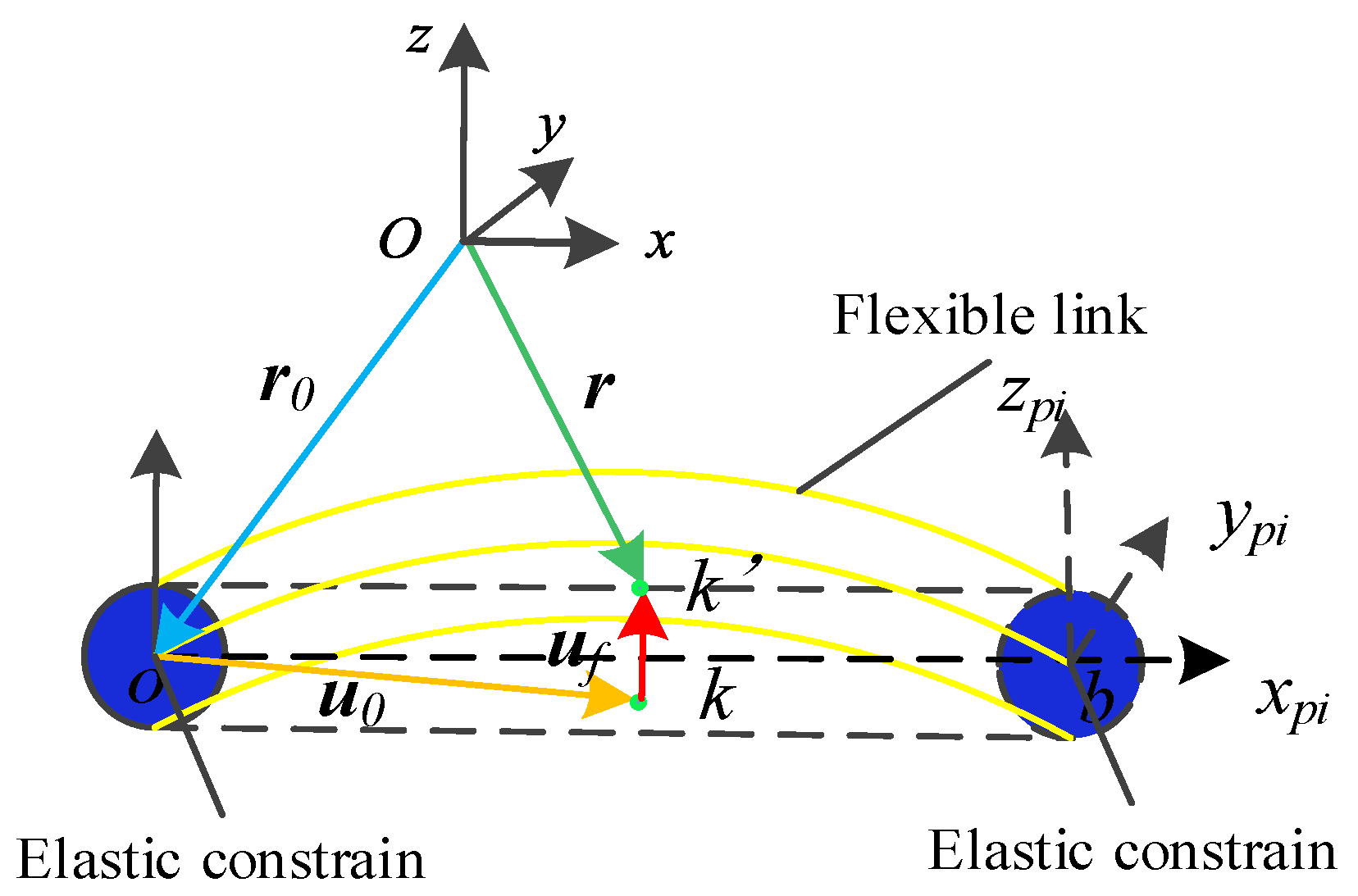
Using a flexible joint as an elastic constraint of a flexible link.

(2)

The flexible link and joint system are simplified as multi-flexible-body systems of two flexible components and a simply supported beam with unilateral elastic constraints.

(3)

The connection between the flexible joint and the rigid link adopts a rigid constraint connection.

(4)

The axis of the flexible joint is coaxial with the rotational axis of the connecting link.

Figure 3 shows a flexible link model with unilateral elastic constraints. In particular, Figure 3 shows that by making the rigid joint flexible, the system’s degrees of freedom can be reduced, and the numerical solution efficiency improved. Simultaneously, the model considers the effect of flexible elastic deformation of the link and joint on the system and the effect of coupling effects between the flexible joint and the rigid.

Due to the flexibility characteristics of flexible joints, the generated joint torque satisfies the relationship ${\mathit{\tau }}_i={\mathit{K}}_{jiont}({\mathit{\theta }}_{jiont}-\mathit{\theta })$, which can be considered as joint stiffness. The dynamic equation of the flexible joint can be obtained according to the first type of Lagrange equation, as follows:

$${\mathit{J}}_{jiont}{\ddot{\mathit{\theta }}}_{jiont}+{\mathit{K}}_{jiont}\left({\mathit{\theta }}_{jiont}-\mathit{\theta }\right)={\mathit{\tau }}_{jiont}$$

(1)

where the rotation matrix and moment of inertia matrix of flexible joints 1 and 2 are ${\mathit{\theta }}_{jiont}=\left[\begin{array}{cc}{\mathit{\theta }}_{i-1j}& {\mathit{\theta }}_{i-2j}\end{array}\right]$ and ${\mathit{J}}_{jiont}=\left(\begin{array}{cc}{\mathit{J}}_{i-1j}& {\mathit{J}}_{i-2j}\end{array}\right)$, respectively, the torsional stiffness of the flexible joint is ${\mathit{K}}_{jiont}=\left(\begin{array}{cc}{\mathit{K}}_{i-1j}& {\mathit{K}}_{i-2j}\end{array}\right)$, the output torque of the flexible joint is ${\mathit{\tau }}_{jiont}$, and i = 1, 2, 3 represents the number of kinematic chains.

The kinetic energy at the flexible joint is as follows:

$$\left\{\begin{array}{c}{T}_{1j}=\frac{{\mathit{J}}_{1j}{\mathit{\omega }}_{{}_{{\mathit{\theta }}_{1i}}}^2}{2}\\ T_{2j}=\frac{{\mathit{J}}_{2j}{\mathit{\omega }}_{{}_{{\mathit{\theta }}_{2i}}}^2}{2}\end{array}\right.$$

(2)

where the angular velocities of flexible joints 1 and 2 are ${\mathit{\omega }}_{{\mathit{\theta }}_{1i}}={\dot{\mathit{\theta }}}_{1j}{}_z$ and ${\mathit{\omega }}_{{\mathit{\theta }}_{2i}}={\dot{\mathit{\theta }}}_{2i}z$, respectively, and z is an intermediate variable.

The potential energy of the flexible joint is as follows:

$$V_{jiont}=\frac{1}{2}{\displaystyle \sum _{i=1}^2{\mathit{K}}_i{}_j\left(\mathit{\theta }-{\mathit{\theta }}_{jiont}\right)}$$

(3)

3.2. Dynamic Modeling of Flexible Link

The sketch of a kinematic chain coordinate system is shown in Figure 4.

Furthermore, the flexible link is in a fixed state owing to the gravity effect. Therefore, when modeling its dynamics, the influence of gravity effect on the system cannot be ignored.

The displacement field vector of any point k on the driven rod can be expressed as follows:

$${\mathit{r}}_k=r_0+T\left({\mathit{u}}_0+{\mathit{u}}_f\right)$$

(4)

where r₀ represents the displacement field vector of the origin of the driven link coordinate system in the global coordinate system,T represents the rotation matrix of the driven link coordinate system transformed into the global coordinate system, and u₀ and u_f = Nq_f represent the coordinate vector of the driven link under and after deformation, respectively. N and q_f represent the shape function and generalized coordinates of the flexible element, respectively. Among them, the generalized coordinates contain three displacement coordinates and three rotation coordinates, respectively. Their deformation modes are described by a first polynomial equation and a cubic polynomial equation. The specific expression is as follows:

$${\mathit{q}}_f=[\underset{node k}{\underbrace{\begin{array}{cccccc}{x}_k& y_k& z_k& {\mathit{\theta }}_{kx}& {\mathit{\theta }}_{ky}& {\mathit{\theta }}_{kz}\end{array}}} \underset{node w}{\underbrace{\begin{array}{cccccc}{x}_w& y_w& z_w& {\mathit{\theta }}_{wx}& {\mathit{\theta }}_{wy}& {\mathit{\theta }}_{wz}\end{array}}}]$$

(5)

According to the kinetic energy expression, the kinetic energy of the flexible link [18] is as follows:

$$T_{cipi}=\frac{1}{2}{\displaystyle \underset{V}{\int }\rho {\dot{r}}_k^T{\dot{r}}_{k}dV+}\frac{1}{2}{\displaystyle {\int }_0^{l_{cipi}}{\dot{\mathit{\theta }}}_{i3}^2}d{J}_c$$

(6)

where $\rho$ and J_c $J_c$ are the density and moment of inertia of the flexible link, respectively. l_cipi and θ_i3 are the length and angle of the flexible link, respectively.

Similarly, the potential energy of a flexible link [18] can be expressed as follows:

$$V_{cipi}=\frac{1}{2}E{\displaystyle {\int }_0^{l_{c_i{p}_i}}\left[A\left(\frac{\partial {\mathit{u}}_f}{\partial x}\right)+I_{zz}{\left(\frac{\partial {\mathit{u}}_f}{\partial x^2}\right)}^2+I_{yy}{\left(\frac{\partial {\mathit{u}}_f}{\partial x^2}\right)}^2\right]}+\frac{1}{2}G{I}_p{\displaystyle {\int }_0^{l_{c_i{p}_i}}\left(\frac{\partial {\psi }_x{\mathit{q}}_f}{\partial x}\right)}$$

(7)

where A and E are the cross-sectional areas and the elastic modulus of the flexible element, respectively. The shear modulus is G, and the moment of inertia functions of the cross-section of the flexible link on the y-axis and z-axis are I_yy and I_zz, respectively. The polar moment of inertia function of the cross-section of the flexible link on the x-axis is I_p, and the elastic rotation function of the flexible link around the x-axis is ${\psi }_x$.

Because the displacement field vector r of the flexible link is known, the gravitational potential energy of the flexible link can be calculated based on the energy theorem. The specific expression is as follows:

$$V_{c_i{p}_i-g}=m_{c_i{p}_i}g\cdot \left[\begin{array}{ccc}0& 0& 1\end{array}\right]\cdot r_k$$

(8)

where m_cipi is the mass of the flexible link.

3.3. Dynamic Modeling of Rigid Links

The length and diameter of the drive rod and intermediate link are relatively small, and the flexible deformation generated during the system movement is ignored. Therefore, analyzing this link as rigid is practical. According to Figure 4, when the drive rod rotates around the axis y_ai, there is only rotational kinetic energy. Moreover, the involved angle is ${\mathit{\theta }}_{i1}$. In contrast, the intermediate link has rotational and translational kinetic energy, and its rotating axis is y_bi. The involved angle is ${\mathit{\theta }}_{i2}$, and the kinetic energy of the rigid link can be calculated as follows:

$$\left\{\begin{array}{l}{T}_{aibi}=\frac{1}{6}{m}_{{}_{aibi}}{l}_{{}_{aibi}}^2{\dot{\mathit{\theta }}}_{i1}^2\\ T_{bici}=\frac{1}{2}{m}_{{}_{bici}}{l}_{{}_{aibi}}^2{\dot{\mathit{\theta }}}_{i1}^2+\frac{1}{6}{m}_{{}_{bici}}{l}_{{}_{bici}}^2{\dot{\mathit{\theta }}}_{i1}^2+\frac{1}{2}{m}_{{}_{bici}}{l}_{{}_{aibi}}{l}_{{}_{bici}}{\dot{\mathit{\theta }}}_{i1}{\dot{\mathit{\theta }}}_{i2}\cos ({\mathit{\theta }}_{i2})\end{array}\right.$$

(9)

where m_aibi and m_bici are the masses of the drive link and intermediate link, respectively. In addition, l_aibi and l_bici are the lengths of the drive and intermediate link, respectively.

Similarly, the potential energy of the rigid link is as follows:

$$\left\{\begin{array}{l}{V}_{aibi}=-\frac{1}{2}{m}_{{}_{aibi}}g{l}_{{}_{aibi}}\sin ({\mathit{\theta }}_{i1})\\ V_{bici}=-\frac{1}{2}{m}_{{}_{bici}}g{l}_{{}_{bici}}\sin ({\mathit{\theta }}_{i1})-\frac{1}{2}{m}_{{}_{bici}}g{l}_{{}_{bici}}\sin ({\mathit{\theta }}_{i2})\end{array}\right.$$

(10)

The end-effector produces a small elastic displacement under the flexible joint 2. Thus, establishing a dynamic equation of the end-effector considering the small displacement is required. Therefore, based on the coordination matrix and boundary conditions, the actual displacement of the rigid end-effector in the global coordinate system can be written as follows:

$$p’=p+J_p\mathsf{\Delta }p$$

(11)

Moreover, the kinetic and potential energies [19] of the end-effector can be written as follows:

$$\left\{\begin{array}{l}{T}_p=\frac{1}{2}{(\dot{p}\prime )}^T{m}_p\dot{p}\prime +\frac{1}{2}{J}_p{w}_p^T\\ V_p=m_{p}g{p}_z\end{array}\right.$$

(12)

where m_p and w_p are the mass and absolute angular velocity of the end-effector, respectively, and $p=\left[\begin{array}{ccc}{p}_x& p_y& p_z\end{array}\right]$ is the displacement vector of the end-effector in the global coordinate system. The displacement of the end-effector in the z-axis direction in the global coordinate system is p_z’.

The coordination matrix [19] J_p can be written as follows:

$$J_p=\left[\begin{array}{cccccc}1& 0& 0& 0& p_z& -p_y\\ 0& 1& 0& -p_z& 0& p_x\\ 0& 0& 1& p_y& -p_x& 0\end{array}\right]$$

(13)

3.4. Dynamic Modeling of Multiple Flexible Kinematic Chains

The dynamic model of the kinematic chain can be obtained by assembling the dynamic models of flexible links, flexible joints, and rigid links. The kinetic and potential energies of the kinematic chain are as follows:

$$\left\{\begin{array}{l}{T}_i=\underset{rigid link}{\underbrace{T_{a_i{b}_i}+T_{b_i{c}_i}}}+\underset{flexible link and jiont}{\underbrace{T_{1j}+T_{c_i{p}_i}+T_{2j}}}\\ V_i=\underset{rigid link}{\underbrace{V_{a_i{b}_i}+V_{b_i{c}_i}}}+\underset{flexible link and jiont}{\underbrace{V_{jionts}+V_{c_i{p}_i}+V_{c_i{p}_i-g}}}\end{array}\right.$$

(14)

3.5. Multi-Flexible-Body Robot System

The inverse dynamics model of multi-flexible-body robots is as follows. First, the generalized coordinates $q_{}=[{\mathit{\theta }}_{\mathrm{i}1} {\mathit{\theta }}_{\mathrm{i}2} {\mathit{\theta }}_{\mathrm{i}3} {\mathit{\theta }}_{\mathrm{i}-1j} {\mathit{\theta }}_{\mathrm{i}-2j} q_f]$ are defined. Then, the total kinetic and potential energies of the system can be obtained by summing the kinetic and potential energies of the flexible links, flexible joints, rigid links, and end-effector. The inverse dynamic model of a multi-flexible-body robot system can be deduced from the derivative of the generalized coordinates, velocities, and accelerations as follows:

$$\left.\left|\frac{d}{dt}(\frac{\partial (T-V)}{\partial \dot{q}})-\frac{\partial (T-V)}{\partial q}=\tau \right.\right|$$

(15)

where $\tau$ is the system driving torque. T and V are the total kinetic and potential energy of the system, respectively.

3.6. Algorithm of Multi-Flexible-Body Robot System

The algorithm for the dynamic model of the multi-flexible-robot system is as follows:

Step 1. Set the system parameters according to the system environment of the multi-flexible-body robots, as shown in

Table 1. Parameters of the multi-flexible-body spatial parallel robot.

Parameter	Mass/kg	Length/m	Density(kg/m3)	Poisson’s Ration	Elastic Modulus/(Pa)
Driving link	2	0.4	7801	0.29	2.07 × 1011
Intermediate link	0.3	0.1	7801	0.29	2.07 × 1011
Flexible link	1.5	0.8	2740	0.33	2.07 × 1011
End-effector	2.6	0	7801	0.29	2.07 × 1011
Flexible joint	0.07	0.04	2740	0.33	2.07 × 1011

.

The dynamic model of the flexible joint with only generalized coordinates can be derived based on the system parameters, initial position, and attitude of the fully rigid mode.

Step 2: Derive the shape function N of the flexible link element and the generalized coordinate q_f of the flexible element as follows:

$$\left\{\begin{array}{c}N=\left[\begin{array}{ccc}{N}_a& N_b& N_c\end{array}\right]\\ q_f=\left[\begin{array}{c}{\mathit{u}}_0-y\frac{\partial v_0}{\partial x}-z\frac{\partial w_0}{\partial x}\\ v_0\\ w_0\end{array}\right]\end{array}\right.$$

(16)

where N_a is the axial interpolation function of the flexible element, and N_b and N_c are the lateral interpolation functions of the flexible element. In addition, u₀, v₀, and w₀ are the axial and torsional deformations of the flexible link relative to the three coordinate axes of the floating coordinate system.

Step 3: Calculate boundary conditions. Flexible joint 1 is connected to the rigid and flexible links. The rigid coordinate of its hinge joint c_i is equal to the flexible coordinate. If one end of flexible joint 2 is connected to the flexible link and the other end to the end-effector, the coordinates of flexible joint 2 should be consistent with the coordinates of the flexible link. Then, the end-effector generates an elastic displacement driven by the flexible joint. The specific model constraints to improve the accuracy of the model solution can be expressed as follows:

$$\left\{\begin{array}{c}{\mathit{u}}_{pi}=J{\mathit{u}}_p\\ c_{i-jiont}=c_{i-flexible}\\ p_{i-jiont}=p_{i-flexible}\end{array}\right.$$

(17)

where c_i-jiont and c_i-flexible are the coordinate vectors of the flexible joint and link under the global coordinates of the hinge joint c_i. Hinge point p_i is equivalent to two coordinate vectors for the model constraints. The motion pairs used between the components of multi-flexible-body robot systems are listed in

Table 2. Constraint relationship.

Kinematic Pair	Component
Rotating pair	Driving link, fixed platform
Rotating pair	Intermediate link, driving link
Rotating pair	Driven link, intermediate link
Hook hinge	Moving platform, driven link

.

Step 4: Assemble the kinetic and potential energies of each component in the kinematic chain to obtain the kinematic chain and system dynamics models according to the triangular symmetry relationship between the kinematic chains.

Step 5: Set the precision for the system’s solution. If the solution settings are satisfied, the next iteration is performed. Otherwise, the system equations are modified according to the constrained default stability method in [20] until all numerical solutions are obtained.

$$\left\{\begin{array}{l}{c}_q\dot{q}+c_t=0\\ c_q\ddot{q}+{[c_q\dot{q}]}_{q}q+2c_{qt}\dot{q}+c_{tt}=0\end{array}\right.$$

(18)

where c_q represents the partial derivative of constraint equation c to the generalized coordinate q, c_qt represents the second derivative of constraint equation c to q at time t, and c_qq represents the second derivative of time t.

The dynamic equations are solved numerically using the acceleration equation. Nevertheless, their cumulative errors gradually increase over time, resulting in non-convergence of the position and velocity constraint equations. Therefore, the constraint equation should be modified as follows:

$${\overline{c}}_{\overline{q}}\overline{q}={\left({\overline{c}}_{\overline{q}}\dot{\overline{q}}\right)}_{\overline{q}}\dot{\overline{q}}+2{\overline{c}}_{\overline{q}t}\dot{\overline{q}}+{\overline{c}}_{tt}-2\alpha {\epsilon }_2-{\beta }^2{\epsilon }_1$$

(19)

where $\alpha$ and $\beta$ are system feedback controls parameters, ε₁ and ε₂ represent the displacement and velocity constraint stabilization parameters, respectively. The expression can be written as follows:

$$\left\{\begin{array}{l}{\epsilon }_1=\overline{c}\\ {\epsilon }_2={\overline{c}}_{\overline{q}}\dot{\overline{q}}+{\overline{c}}_t\end{array}\right.$$

(20)

4. Inverse Dynamics Simulation Model of Multi-Flexible-Body Robots

4.1. Rigid Simulation Model Validation

The correctness of the developed simulation model was verified by establishing the correct model of a fully rigid spatial parallel robot. Therefore, all components were designated as rigid components. Moreover, because the driven link is a spatial one, both translational and rotational kinetic energy exists. Therefore, according to the kinetic energy formula, the kinetic and potential energies of the driven link considered as a rigid body are as follows:

$$\left\{\begin{array}{l} T_{{\mathrm{c}}_i{p}_i-r}=\frac{1}{2}{J}_{c_i{p}_i}{\dot{\mathit{\theta }}}_{i3}^2\\ T_{c_i{p}_i-t}=\frac{1}{2}{m}_{c_i{p}_i}{\left[\left(a_i{b}_i+b_i{c}_i+\frac{1}{2}{c}_i{p}_i\right)\right]}^2\\ V_{c_i{p}_i}=-m_{c_i{p}_i}g{l}_{a_i{b}_i}\sin ({\mathit{\theta }}_{i1})-m_{c_i{p}_i}g{l}_{b_i{c}_i}\sin ({\mathit{\theta }}_{i2})-\frac{1}{2}{m}_{c_i{p}_i}g{l}_{c_i{p}_i}\sin ({\mathit{\theta }}_{i2})\cos ({\mathit{\theta }}_{i3})\end{array}\right.$$

(21)

where T_cipi-r is the rotational potential energy of the driven link, and T_cipi-t is the translational kinetic energy of the driven link. The rotational inertia of the driven link in the global coordinate system is J_cipi.

Simultaneously, the kinetic energy and potential energy of the end-effector without the effect of flexible deformation can be derived from the momentum theorem as follows:

$$\left\{\begin{array}{l}{T}_p=\frac{1}{2}{m}_P({\dot{p}}_x^2+{\dot{p}}_y^2+{\dot{p}}_z^2)\\ V_p=-m_{P}g{p}_z\end{array}\right.$$

(22)

The dynamic equation of the fully rigid spatial parallel robot can be obtained by substituting Equations (9), (10), (21), and (22) into Equation (15).

Moreover, the motion trajectory of the end-effector is assumed as follows:

$$\left\{\begin{array}{l}{p}_x=0.1\cos (\omega \cdot t)\\ p_y=0.1\sin (\omega \cdot t)\\ p_z=-0.7\\ \omega =2 \mathrm{rad}/s\end{array}\right.$$

(23)

Based on the derived dynamic equation of the fully rigid spatial parallel robot, the transformation relationship between the driving torque of the three kinematic chains and the time can be obtained, as shown in Figure 5.

Furthermore, the correctness of the derived dynamic equations of the fully rigid spatial parallel robot (Figure 1) was verified against a three-dimensional model developed in SOLIDWORKS, saved in (x_t) format, and imported into the simulation software ADAMS. Finally, the ADAMS model was used to develop a fully rigid spatial parallel robot simulation model. The specific modeling process was as follows:

• Add the properties of each system component according to the values listed in Table 1. Then, add the constraint relationships between each component according to Table 2.
• Use the point drive motion in the ADAMS/Force module to load the motion trajectory given by Equation (23) to the geometric center of the end-effector. A running time of 5 s and a step size of 0.005 s was set for the simulation. By using inverse dynamics simulation, the variation relationship of each driving torque of the kinematic with time could be obtained, as shown in Figure 6.

Figure 5 shows that due to the triangular symmetric distribution of the kinematic chain, the curves representing the three driving torques corresponding to the driving components are uniformly distributed, and the curves are smooth. This result indicates the good dynamic performance of the system. Furthermore, the comparison of the numerical results in Figure 5 and Figure 6 indicates that the driving torque motion trends of the numerical and simulation models are consistent, verifying their correctness. However, due to aspects in the assembly process of the simulation model, such as assembly errors and joint clearances, the driving torque values are greater than that of the numerical model, which is consistent with the actual situation.

4.2. Verification of Multi-Flexible-Body Simulation Model

The correctness of the simulation model of the multi-flexible-body spatial parallel robot can be verified by establishing a flexible model starting from a fully rigid spatial parallel robot simulation model. Then, the results of the built model and the numerical results can be compared.

The flexibility in the driven links and joints in the fully rigid spatial parallel robot shown in Figure 1 can be included using the Admas/Flex module. That is, the multi-flexible-body robot simulation model can be obtained by adding constraint relationships of each component according to Table 2. The constraint models of flexible links, flexible Hooke hinges, and the rigid end-effector are shown in Figure 7.

The equivalence between the simulated and real model was ensured by retaining the first six modal component information during the process of modeling flexible components and introducing the motion pair information of the flexible joint and link under the boundary conditions. The simulation model of the multi-flexible-body robots is shown in Figure 8. After including flexibility, the flexible joint generated 108 nodes and 317 units, and the flexible link generated 1123 nodes and 2349 units.

Before the simulation, the model constraints and degrees of freedom were validated to verify model accuracy. The simulation results showed that the degrees of freedom of the model are consistent with the theoretical calculation, indicating that the model constraint relationship was correct. The GSTIFF integrator and SI2 integration format in ADAMS were selected to ensure calculation efficiency and accuracy during simulation. The simulation time was set to 5 s, the time interval was 0.005 s, the solution accuracy was 10⁻⁴, and the simulation type was dynamic. Subsequently, the rigid robot dynamics result [20] was obtained, considering that the robot was driven following a spline function in the driving joints. The specific function is as follows:

$$\left\{\begin{array}{c}CUBSPL\left(\begin{array}{cccc}time,& 0,& Spline1,& 0\end{array}\right)\times 1d\\ CUBSPL\left(\begin{array}{cccc}time,& 0,& Spline2,& 0\end{array}\right)\times 1d\\ CUBSPL\left(\begin{array}{cccc}time,& 0,& Spline3,& 0\end{array}\right)\times 1d\end{array}\right.$$

(24)

The obtained dynamic results can be compared with those of the rigid robot. The initialization results for the multi-flexible-body spatial robot are shown in Figure 9.

5. Simulation Analysis

The dynamic characteristics of the multi-flexible-body spatial parallel robot were accurately analyzed by comparing the forward dynamic characteristics of the fully rigid dynamic model and the multi-flexible-body spatial parallel robot under the same driving conditions. The change law of the driving torque under different angular velocities was analyzed using the reverse dynamic model.

5.1. Positive Dynamics Analysis of the Multi-Flexible-Body Robot

Based on Equation (24), a positive dynamics analysis of the multi-flexible-body spatial parallel robot was conducted. The geometric center of the end-effector is plotted as a circular trajectory at p_z = 0.7 m under the action of the driving torques, as shown in Figure 10.

To visually analyze the effect of flexible joints and links on the motion trajectory of the end-effector, the motion curves of the end-effector of the multi-flexible-body spatial parallel robot and the full rigid spatial parallel robot in the X-, Y-, and Z-axes were compared. The results are shown in Figure 11, Figure 12 and Figure 13.

The motion trajectory of the multi-flexible-body spatial parallel robot in the X, Y, and Z directions is the same as that of the full rigid spatial parallel robot. However, due to the elastic deformation generated during the movement of flexible joints and links, the end effector will have a small displacement. Therefore, its motion trajectory floats around the motion trajectory of the fully rigid spatial parallel robot within a certain range. Among them, the range of travel of the multi-flexible-body spatial parallel robot model in the X, Y, and Z directions is 0–3.14, 0–4.06, and 0–0.483 mm, respectively. Therefore, the elastic deformation of flexible links and joints and the coupling between flexible joints and rigid links, and between flexible joints and links considerably affect the motion trajectory of the system’s end-effector. Therefore, it is important to establish a dynamic model that conforms to the characteristics of multi-flexible-body systems.

By substituting Equations (14) and (19) into Equation (15), the numerical solution of the dynamic model of the multi-flexible-body spatial parallel robot can be derived. Moreover, the correctness of the numerical model of the multi-flexible-body spatial parallel robot can be ensured by comparing its results with those of the simulation model, as shown in Figure 14, Figure 15 and Figure 16.

Figure 14, Figure 15 and Figure 16 show that the motion trends of the end effectors of the numerical model and simulation model of the multi-flexible-body spatial parallel robot are consistent on the three coordinate axes x, y, and z. However, because the numerical model is a highly nonlinear, strongly coupled, and time-varying differential algebraic equation, its solution accuracy depends on the numerical algorithm and convergence accuracy settings.

Among them, the range of travels of the numerical model in the x-, y-, and z-directions are 0 to 4.43, 0 to 5.61, and 0 to 0.81 mm, respectively. In addition, control strategy analysis can be conducted based on numerical solutions to improve the control performance of the system. Simultaneously, simulating the control system and trajectory tracking accuracy through simulation models facilitates control system debugging and reduces production costs.

5.2. Inverse Dynamics Analysis of Multi-Flexible-Body Robots

During the system operation, the angular velocity significantly affects the vibration characteristics of the mechanism, the deformation degree of the links, and the change in the driving torque. Therefore, we investigate the system’s dynamic characteristics by analyzing the change law of the driving torque under different angular velocities using an inverse dynamics model. According to actual working conditions, the angular velocity is generally 1.5–2.5 rad/s. Therefore, the angular velocity was set as ω = 1.8 and 2 rad/s. The geometric center motion of the end effector was set according to Equation (23).

An inverse dynamics analysis of multi-flexible-body spatial parallel robots was performed using the Adams/Motion module, considering that the geometric center of the end-effector moves according to Equation (23). The variation law of the driving torque of each kinematic chain of the multi-flexible-body spatial parallel robots under different angular speeds is shown in Figure 17 and Figure 18.

With increasing angular velocity, the maximum absolute amplitude of the driving torque of each kinematic chain also increases. In contrast, its motion trend remains unchanged. The maximum driving torques of motion chains 1, 2, and 3 at an angular velocity of 1.8 rad/s are 3.21, 1.83, and 0.97 N m, respectively, and equals 3.62, 1.95, and 1.06 N m, respectively, at an angular velocity of 2 rad/s. By analyzing the inverse dynamics model of the multi-flexible-body spatial parallel robot under different angular velocities, the change law of the system driving torque can be obtained, providing a data reference for the rational selection of driving components.

6. Conclusions

By solving and analyzing the multi-body dynamics equations of a multi-flexible-body spatial parallel robot considering flexible links and joints, we conclude the following:

(1)

In this paper, a multi-flexible-body spatial parallel robot was numerically simulated through a co-simulation between ADAMS and SOLIDWORKS. The correctness of the derived dynamic equations and the effectiveness of the simulation mode were verified. The simulation results were consistent with the actual working conditions.

(2)

The elastic deformation of flexible joints and links in the motion process considerably affects the motion trajectory of the system’s end-effector. Therefore, the flexibility of the links and joints cannot be ignored when establishing an accurate dynamic model for a multi-flexible-body spatial parallel robot.

(3)

During the system operation, the coupling effect between the flexible joint and rigid link and between the flexible joint and flexible link is complex. Therefore, the effect of the higher-order mode on the motion trajectory of the system should be considered.

The constraint relationship of the simulation model and its inverse dynamics results were consistent with the motion trend of a fully rigid spatial parallel robot. Moreover, simulating the control system and trajectory tracking accuracy through simulation models facilitates control system debugging and reduces production costs.

Therefore, this study provides a scientific basis for investigating the dynamic characteristics of a multi-flexible-body spatial parallel robot through a simulation model.

References

1. Fang, W.Y.; Guo, X.; Liang, L.; Zhang, D. Dynamics, simulation, and control of robots with flexible joints and flexible links. Chin. J. Theor. Appl. Mech. 2020, 54, 965–974. (In Chinese) [Google Scholar]
2. Zhang, F.L.; Yuan, Z.H. Flexible space robot modeling and characteristic analysis based on Recursive Gibbs-Appell. J. Aerosp. Power 2020, 1–16. [Google Scholar] [CrossRef]
3. Zhang, Q.; Mills, J.K.; Cleghorn, W.L.; Jin, J.; Zhao, C. Trajectory and vibration suppression of a 3-PRR parallel manipulator with flexible links. Multibody Syst. Dyn. 2015, 33, 27–60. [Google Scholar] [CrossRef]
4. Ssyahkarajy, M.; Mohamed, Z.; Mohd Faudzi, A.A. Review of modelling and control of flexible-link manipulators. Proc. Inst. Mech. Eng. Part I J. Syst. Control Eng. 2016, 230, 861–873. [Google Scholar] [CrossRef]
5. Virgili-Llop, J.; Drew, J.V.; Zappulla II, R.; Romano, M. Laboratory experiments of resident space object capture by a spacecraft- manipulator system. Aerosp. Sci. Technol. 2017, 71, 530–545. [Google Scholar] [CrossRef]
6. Korayem, M.H.; Dehkordi, S.F.; Mehrjooee, O. Nonlinear analysis of open-chain flexible manipulator with time- dependent structure. Adv. Space Res. 2022, 69, 1027–1049. [Google Scholar] [CrossRef]
7. Gouliaev, V.I.; Zavrazhina, T.V. Dynamics of a flexible multi-link cosmic robot- manipulator. J. Sound Vib. 2001, 243, 641–657. [Google Scholar] [CrossRef]
8. Shafei, A.; Shafei, H. Oblique impact of multi- flexible- link systems. J. Vib. Control 2016, 2, 25–34. [Google Scholar] [CrossRef]
9. Hu, J.F.; Zhang, X.M.; Zhu, D.C.; Chen, Q. Dynamic modeling of flexible parallel robot. Trans. Chin. Soc. Agric. Mach. 2011, 42, 208–213. [Google Scholar]
10. Li, L.; Liu, Z.Y.; Hong, J.Z. Model reduction of rigid-flexible coupling dynamics of hub-beam system. J. Econ. Dyn. Control 2015, 13, 6–10. [Google Scholar]
11. Meng, D.; She, Y.; Xu, W.; Lu, W.; Liang, B. Dynamic modeling and vibration characteristics analysis of flexible-link and flexible-joint space manipulator. Multibody Syst. Dyn. 2018, 43, 321–347. [Google Scholar] [CrossRef]
12. Fu, X.; Chen, L. Output feedback finite-dimensional repetitive learning control on virtual force link and flexible-joint space robot. Chin. J. Space Sci. 2021, 41, 819–827. (In Chinese) [Google Scholar]
13. Zhang, X.Y.; Liu, X.F.; Cai, G.P.; Liu, C.K. Dynamic modeling of a flexible-link flexible-joint manipulator. J. Econ. Dyn. Control 2022, 20, 25–39. [Google Scholar]
14. Kunming, Z.; Youmin, H.; Wenyong, Y. A novel parallel recursive dynamic modelling method for robot with flexible bar-groups. Appl. Math. Model 2020, 77, 267–288. [Google Scholar]
15. Wang, J. Modified models for revolute joints coupling flexibility of links in multibody systems. Multibody Syst. Dyn. 2019, 45, 37–55. [Google Scholar] [CrossRef]
16. Zhang, Q.; Zhao, X.; Liu, L.; Dai, T. Dynamics analysis of spatial parallel robot with rigid and flexible links. Math. Biosci. Eng. 2020, 17, 7101–7129. [Google Scholar] [CrossRef] [PubMed]
17. Spong, M.W. Modeling and control of elastic joint robots. J. Dyn. Syst. Meas. Control 1987, 109, 310–319. [Google Scholar] [CrossRef]
18. Zhang, Q.Y.; Zhao, X.H.; Liu, L.; Dai, T.D. Adaptive sliding mode neural network control and flexible vibration suppression of a flexible spatial parallel robot. Electronics 2021, 10, 212. [Google Scholar] [CrossRef]
19. Huang, Z.; Kong, L.F.; Fang, Y.F. Mechanism Theory and Control of Parallel Robot; Machinery Industry Press: Beijing, China, 1997. [Google Scholar]
20. Zhang, Q.Y. Research on Nonlinear Mathematical Modeling and Intelligent Control Algorithm of Flexible Spatial Closed—Chain Robot; Tianjin University of Technology: Tianjin, China, 2021. [Google Scholar]
Figure 1. Multi-flexible-body spatial parallel robot.
Electronics 12 02038 g001
Figure 2. Structure diagram of the multi-flexible-body kinematic chains.
Electronics 12 02038 g002
Figure 3. Model of the flexible link with an elastic constraint.
Electronics 12 02038 g003
Figure 4. Coordinate system diagram of a kinematic chain.
Electronics 12 02038 g004
Figure 5. Driving torque obtained from the numerical models.
Electronics 12 02038 g005
Figure 6. Driving torque of the simulation models.
Electronics 12 02038 g006
Figure 7. Simulation model of a flexible Hooke hinge.
Electronics 12 02038 g007
Figure 8. Simulation model of the multi-flexible-body spatial parallel robot.
Electronics 12 02038 g008
Figure 9. Initialization model of the multi-flexible-body spatial parallel robot.
Electronics 12 02038 g009
Figure 10. Trajectory of the end-effector.
Electronics 12 02038 g010
Figure 11. Displacement in the x-direction of the end-effector.
Electronics 12 02038 g011
Figure 12. Displacement in the y-direction of the end-effector.
Electronics 12 02038 g012
Figure 13. Displacement in the z-direction of the end-effector.
Electronics 12 02038 g013
Figure 14. Displacement in the x-direction of the end-effector.
Electronics 12 02038 g014
Figure 15. Displacement in the y-direction of the end-effector.
Electronics 12 02038 g015
Figure 16. Displacement in the z-direction of the end-effector.
Electronics 12 02038 g016
Figure 17. Driving torque at ω = 1.8 rad/s.
Electronics 12 02038 g017
Figure 18. Driving torque at ω = 2 rad/s.
Electronics 12 02038 g018