Abstract
In the polar region, the gravity vector and Earth’s rotation vector tend to be in the same direction, leading to a slower convergence speed and longer alignment time of the moving base alignment. When the alignment time is short, the alignment cannot converge, resulting in low azimuth accuracy. To address this issue, we propose a polar moving base alignment method based on a backtracking scheme. Notably, this work first derives a polar coarse alignment method with the inertial frame based on the transverse Earth model. On this basis, we designed a polar coarse alignment method based on a backtracking scheme and optimized the data storage scheme. Then, a backward navigation algorithm based on the transverse inertial navigation mechanical arrangement scheme was derived, and a polar fine alignment method based on a backtracking scheme was designed. Semi-physical simulation experiments showed that the alignment algorithm based on a backtracking scheme could converge in the 180 s with high alignment accuracy, which is 70% faster than the current polar moving base alignment method.
1. Introduction
In recent years, global warming has accelerated the melting of polar ice caps, leading to an increase in the value of strategic, economic, scientific, environmental, navigational, and resources in the polar region [1]. To achieve smooth and safe navigation or operations in the polar region, various types of marine carriers must rely on high-precision navigation systems [2]. The high-precision strapdown inertial navigation system (SINS) has become the core navigation technology to meet the application of polar regions with its autonomy and resistance to external environmental interference [3]. As one of the key technologies of the SINS, a moving base alignment is also a research hotspot in the field of polar navigation.
Auxiliary navigation information is necessary to achieve the moving base alignment. However, the arctic geophysical field may impair electrical or optical-based auxiliary navigation systems [4,5], resulting in performance degradation or even failure, which in turn leads to alignment failure. For example, affected by intense magnetic storms, the accuracy of the Global Navigation Satellite System (GNSS) decreases and sometimes even fails. Moreover, common meteorological conditions in the polar region, such as fog, low clouds, snow, and polar night, limit visibility, which affects the observation of starlight by astronomical navigation sensors, rendering astronomical navigation unusable. In contrast, the Doppler Velocity Log (DVL) is preferred to assist in a moving base alignment since it is not affected by the unique geography of the polar region [6].
The initial alignment process is divided into two stages: coarse alignment and fine alignment [7]. The main task of the coarse alignment is to obtain a rough attitude matrix of the carrier in a short time and provide it to the fine alignment [8]. The fine alignment aims to obtain a high-precision attitude matrix of the carrier, which takes a long time to complete [9].
The coarse alignment of the moving base is usually achieved through the use of inertial alignment methods [10,11,12,13]. In the polar region, the convergence of meridians with increasing latitudes leads to the amplification of longitude errors, which increases the alignment error of traditional inertial alignment algorithms that involve longitude terms in the solution process. To address this issue, Liu proposed a polar inertial frame alignment algorithm with pseudo-SINS modeling, which eliminated the impact of longitude error amplification on the polar alignment [13]. However, the use of a spherical Earth model in the pseudo-SINS modeling leads to the principle error in this alignment algorithm, while the transverse Earth ellipsoid model is an ellipsoidal model, and there is no amplification of errors in the transverse latitude and longitude directions in the polar region [14]. Therefore, we designed a -aided inertial alignment algorithm under the transverse Earth model to eliminate the principle error and the amplification of longitude errors.
During the fine alignment of a moving base, an integrated alignment method is usually used [15,16,17,18,19]. In the polar region, as the latitude increases, the gravity vector and Earth’s rotation vector tend to be in the same direction, the gyrocompass effect weakens, and the azimuth accuracy of the coarse alignment of the inertial system decreases. This results in difficulties in achieving the integrated alignment aided by the DVL under a small misalignment. To address this issue, Wang proposed a DVL-aided integrated alignment algorithm for a large misalignment angle in the polar region [18]. However, linearization was performed when deriving the differential equation of the velocity error, resulting in large azimuth errors in the alignment. Liu re-derived the DVL-aided integrated alignment algorithm under a large azimuth misalignment, which improved the azimuth accuracy [19].
Currently, research on polar alignment algorithms has focused on improving alignment accuracy but not on alignment speed. In order to improve the alignment speed of the SINS, [20,21,22] have proposed integrated fine alignment methods based on a backtracking scheme, which effectively shortens the alignment time. In the polar region, the gyrocompass effect weakens, and the convergence time of the inertial frame coarse alignment is increased, resulting in the coarse alignment time exceeding the backtracking fine alignment time. Therefore, when designing a polar region backtracking alignment algorithm, not only a backtracking fine alignment algorithm needs to be designed, but also a backtracking coarse alignment algorithm needs to be designed to shorten the coarse alignment time. Reference [23] proposed a backtracking coarse alignment algorithm that effectively shortens the coarse alignment time. However, their research was implemented based on the North mechanics arrangement and cannot be directly applied to the polar region. In addition, during the backtracking coarse alignment process, the parameters in the backward coarse alignment update process have already been calculated in the forward coarse alignment update process. Recalculating the parameters using gyroscope and accelerometer data in the backward coarse alignment update process will lead to wasted computational resources. Furthermore, the integrated fine alignment algorithm under a large azimuth misalignment in the polar region can quickly reduce the azimuth error to a small misalignment. Therefore, when designing the polar backtracking fine alignment algorithm, the large azimuth misalignment-integrated fine alignment algorithm only needs to be run once, and a subsequent backtracking fine alignment process can be realized using the small misalignment-integrated fine alignment algorithm.
Based on the above analysis, this paper proposes a moving base backtracking alignment method in the polar region. The main contribution of this paper is the derivation of an auxiliary inertial alignment algorithm under the transverse Earth model, which improves the coarse alignment accuracy in the polar region. On this basis, a polar coarse alignment and fine alignment method based on a backtracking scheme were designed, which shortened the alignment time for both the coarse and fine alignment. The structure of this paper is as follows: Section 2 introduces all the frames involved in the polar backtracking alignment algorithm, derives the polar coarse alignment method with the inertial frame based on the transverse Earth model, and introduces the polar fine alignment algorithm. Section 3 proposes the polar coarse and fine alignment methods based on a backtracking scheme. Section 4 analyzes the experimental results. Finally, Section 5 gives the conclusion.
2. The Polar Coarse and Fine Alignment Methods
In this section, the frames used in the polar coarse and fine alignments are first introduced. Then, the polar coarse alignment method with the inertial frame based on the transverse Earth model is derived to eliminate the effect of the polar alignment algorithm caused by longitude error amplification. Finally, the integrated fine alignment algorithm under a large azimuth misalignment and the integrated fine alignment algorithm under a small misalignment used in the backtracking fine alignment process are, respectively, introduced into the polar region.
2.1. Transverse Earth Model and the Definition of Transverse Frame
The definition of the transverse Earth model and the inertial navigation arrangement in this paper are consistent with reference [14], as shown in Figure 1. In the transverse Earth model, the transverse North Pole is the intersection point between the 90°E meridian and the equator, the transverse equator is the meridian circle composed of the 0° and 180° meridians, and the transverse prime meridian is the meridian circle composed of the 90° E and 90° W meridians. The transverse latitude, , is the angle between the normal of point on the ellipsoid and the transverse equatorial plane, and the transverse longitude, , is the angle between the projection of on the transverse equatorial plane and axis.
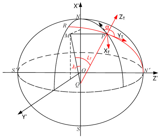
Figure 1.
The transverse ellipsoid Earth model.
Following reference [14], the transformation matrix between the Earth frame and the transverse Earth frame is as follows:
To facilitate subsequent problem description and formula derivation, all frames involved in the algorithm are defined as right-handed Cartesian frames, which are defined as follows:
- The Earth-Centered inertial frame, : the origin, , is at the center of the Earth, the axis points towards the vernal equinox, and the axis points towards the North Pole;
- Earth-Fixed frame, : the origin, , is at the center of the Earth, the axis points to the prime meridian, and the axis points to the North Pole;
- The transverse Earth frame, : the origin, , is at the center of the Earth, the axis points to the transverse prime meridian, and the axis points to the transverse North Pole;
- The transverse geographic frame, : the origin, , is the center of the mass of the carrier. The axis points to the north in the transverse direction, and the axis is perpendicular to the local transverse plane and points to the sky;
- The body frame, : The origin, , is at the center of the mass of the body. The axis points to the right of the body, the axis points forward along the longitudinal axis, and the axis points upward along the body axis;
- The initial transverse inertial frame, : the origin, , is at the center of the Earth, the axis points to the transverse North Pole, and the axis is parallel to the in the transverse equatorial plane;
- The initial transverse Earth frame, : the frame, , at the initial moment;
- The initial transverse geographic frame, : the frame, , at the initial moment;
- The initial body frame, : at the initial moment, the frame, , coincides with the frame, , and after the alignment begins, the frame, , remains fixed and does not move with the body.
Among them, frames , , and remain fixed in the inertial space and do not change with time. Frames , , , and maintain the same orientation as the Earth’s motion. Frames and are fixed to the body.
2.2. The Inertial Frame Coarse Alignment Algorithm Aided by the Based on the Transverse Earth Model
In the polar moving base alignment algorithm, all time-varying variables are represented in . The attitude matrix, , at time , is decomposed into the product of three matrices as follows:
where is the transformation matrix from frame to frame under the horizontal Earth model. is the attitude matrix of frame relative to frame , both of which can be obtained through navigation information. is the attitude matrix of frame relative to frame under the transverse Earth model, which is a constant matrix.
Based on the analysis above, can be obtained as follows:
where and can be obtained from the transverse longitude and latitude of the body’s location, and can be obtained in real-time using the Earth’s rotation rate, , and the transverse longitude, , of the body’s location at the initial moment. is the attitude matrix of frame relative to frame .
where and represent the transverse longitude and latitude of the body location at .
where the initial value of matrix is the identity matrix , i.e., is the change in rotation of frame relative to frame from time to time . is the equivalent rotation vector of frame relative to the reference frame, , from time to time , which can be obtained from the angular velocity, , between frame and frame .
As is always constant, it can be derived that:
where is the duration of period , and is the angular rate of Earth’s rotation. can be obtained by solving from (4)–(9).
Then, can be calculated by the following equation:
where the initial value of matrix is the identity matrix , i.e., can be calculated in real-time through the equivalent rotation vector, .
can be solved using the “single-sample + previous cycle” algorithm with the inertial navigation sampled angle increment, .
According to the matrix decomposition in Equation (2), the calculation of the transformation matrix, , can be converted into the calculation of a fixed matrix, . This transforms a traditional time-varying attitude error estimation problem into a time-invariant attitude error estimation problem.
According to the SINS attitude and velocity update equation, we can obtain:
where is the projection of the angular velocity between frame and frame onto frame , and are the vehicle velocities in frame and frame , respectively, is measured by the DVL, is the output of the ideal accelerometer, is the projection of frame relative to frame onto frame , and and are the projections of the Earth’s rotation rate and gravitational acceleration onto frame .
Taking the derivative of both sides of (15) and substituting (13), we obtain:
By substituting (16) into (14) and simplifying, we obtain:
By substituting (2) into (17) and simplifying, we obtain:
In order to reduce the influence of the DVL velocity measurement errors and accelerometer measurement errors and by integrating both sides of Equation (18) and simplifying, we can obtain the velocity vector observation aided by the DVL velocity, :
where
According to Equation (19), the solution for is converted into a Wahba problem when and are known [24]. For the Wahba problem, the singular value decomposition (SVD) algorithm and quaternion-based methods, such as the q-method, are essentially equivalent in the results, but the SVD algorithm is more concise and intuitive [25]. Therefore, the SVD method is used to solve. The specific solution method is as follows:
where the variable, , represents the end time in the alignment process.
Matrix can be decomposed using SVD as follows:
where is the singular value of matrix .
The attitude transformation matrix can be obtained from this equation:
Due to the unknown before the coarse alignment and the unavailability of real-time position information other than the velocity information provided by the DVL, there are two approximations made in the computation of the constant matrix, , during the moving base coarse alignment process. Firstly, in Equation (4), the initial position information is used as a substitute when calculating . Secondly, in Equation (20), the variable is ignored because is unknown. Therefore, the actual computation of Equations (4) and (20) are as follows:
where variables and represent the initial transverse longitudinal and latitudinal positions of the body, respectively.
However, it should be noted that the approximation in calculating results in relatively large errors. However, in the process of solving in Equation (2), both and contain the error caused by the first approximation, and the errors partially offset each other. As a result, the accuracy of is higher than that of when the coarse alignment is completed.
In summary, the attitude matrix, , can be obtained by using Equations (2)–(12) and (19)–(26) to achieve coarse alignment of the moving base. In the backward process, the initial attitude can be calculated by substituting the obtained from the coarse alignment into Equation (2).
2.3. The Polar Fine Alignment Method Assisted by DVL under Large Azimuth Misalignment
The integrated alignment algorithm assisted by the DVL under a large azimuth misalignment angle used in this paper is consistent with the approach in reference [19]. Based on the nonlinear error equations of transverse inertial navigation, a state model was established. The velocity information from the DVL was used to establish a measurement model. The adaptive unscented Kalman filter (UKF) algorithm was employed to achieve the alignment. The state and measurement models are shown below.
The model can ignore the altitude velocity error, , and height error . The platform misalignment, , transverse horizontal velocity error, , transverse longitude and latitude error, , constant gyro drift, , and accelerometer bias, , were selected as states.
The state equation can be obtained as follows:
where
where represents the attitude matrix between the computed navigation frame and frame , represents the calculated value of the commanded angular velocity, represents the navigation frame calculation error, represents the calculated value of the attitude matrix, represents the output of actual acceleration, represents the calculated value of the projection of Earth’s rotation angular velocity in frame , represents the calculated value of the projection of frame relative to frame in frame , represents the calculation error of Earth’s rotation angular velocity, represents the calculation error of the navigation system rotation angular velocity, represents the calculated value of the carrier velocity in frame , represents the error of the carrier velocity in frame , and represent the calculated values of the transverse latitude and longitude, respectively, and represent the errors of the transverse latitude and longitude, respectively, and represent the calculated values of the transverse eastward and northward velocity, respectively, and represent the attitude angles of the rotation around the x-axis and y-axis, respectively, and represent the curvature radii of the Earth’s meridian and transverse circles, respectively, and represents the angle between frame and the local geographic frame, .
The measurement equation for the difference between the velocity provided by the SINS and DVL in frame is given by:
where and represent the SINS and DVL outputs in frame , respectively. and represent the errors of the SINS and DVL velocity outputs in frame .
2.4. The Polar Fine Alignment Method Assisted by DVL under Small Misalignment
In the integrated alignment algorithm under a small misalignment used in this paper, we established a state model based on the transverse SINS linear error equation and designed a measurement model using the velocity from the DVL. We implemented the alignment using the Kalman filter. The state model is consistent with that in reference [17], and the measurement model is designed as follows.
The model can ignore the altitude velocity error, , and the height error, . The platform misalignment, , transverse horizontal velocity error, , transverse longitude and latitude error, , constant gyro drift, , and accelerometer bias, , were selected as states.
The state equation can be obtained as follows:
In this paper, the measurement equation is given by the difference between the velocity provided by the SINS and DVL in frame . Firstly, the measurement of the DVL was modeled as the superposition of true values and white noise errors while ignoring the items that could be obtained through experimental calibration, such as the scale factor error and installation error of the DVL. The velocity output by the DVL can thus be obtained as:
where represents the actual velocity in frame , and represents the velocity random walk error.
The velocity obtained by the DVL is projected onto frame and denoted as
Ignoring second-order terms, the DVL velocity in frame can be obtained as:
The velocity information output by the transverse SINS is obtained as:
The measurement equation is:
3. The Polar Backtracking Alignment Method
3.1. The Polar Backtracking Coarse Alignment Method
Assuming that the carrier departs from point O at time 0 and arrives at point P at time , the motion process is defined as the forward process, which takes the time. Then, from time to time 0, the carrier moves from point P to point O, and this process is defined as the backward process.
The polar backtracking coarse alignment consists of two parts: one is to complete the forward coarse alignment and store relevant data, and the other is to use the stored data to simulate and generate the data required for the backward coarse alignment process and complete the backward coarse alignment, as shown in Figure 2. It should be noted that the backward coarse alignment algorithm continues to operate based on the forward coarse alignment algorithm rather than being an independent process, as shown in Figure 3. That is to say, the backtracking coarse alignment actually uses the data with a length of achieving alignment through the coarse alignment algorithm.
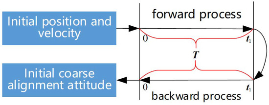
Figure 2.
Timing arrangement of the polar backtracking coarse alignment.
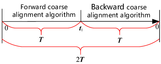
Figure 3.
The running process of the polar backtracking coarse alignment.
The algorithm used in the forward process is directly adopted from Section 2.2 of this paper. However, the solution method for variable in the coarse alignment algorithm used in the backward process is different from that in Section 2.2. The reason for this difference is that at time when the forward process turns to the backward process, the projection of the body’s velocity in the inertial frame undergoes a sudden change from to . However, this velocity change is not reflected in the specific force integration term used in , so compensation needs to be added in . The compensated variable, , is as follows:
Apart from the compensation required for , and other calculations are not affected. That is, the method of obtaining the fixed attitude matrix, , in the backward coarse alignment algorithm is as follows:
where
The solution for can be obtained using Equations (41)–(43), and can be obtained using Equation (2). Furthermore, considering that all the parameters in and have been calculated in the forward coarse alignment to save computational costs and reduce the computational burden, the proposed method for the backtracking coarse alignment in this paper stores the parameter data in and during the forward coarse alignment process and directly provides it to the backtracking coarse alignment process.
It is important to note that when the forward process turns into the backward process, the body frame undergoes a sudden change, rotating 180° around the Z-axis. This means that the transformation matrix, , between frame and frame changes. Therefore, at the backward moment, , the transformation matrix between frame and frame is given by:
where represents the corresponding forward process time of the backward process, ; that is, . is the rotation matrix obtained by rotating counterclockwise 180° around the Z-axis.
In the backward process, except for the calculation of using Equation (44), all parameters in and correspond one-to-one with the corresponding forward process moment. The required data sequence for the backtracking coarse alignment is shown in Table 1.

Table 1.
Data sequence of the polar backtracking coarse alignment.
In summary, the proposed backtracking coarse alignment method consists of the following steps:
- Use the inertial frame coarse alignment algorithm in Section 2.2 to complete the forward coarse alignment and store the parameters in and , the gyroscope, the accelerometer, and the DVL data as the forward data;
- Use the partially stored data in the forward process to simulate the data required for the backward coarse alignment process, as detailed in Table 1;
- Continue the forward coarse alignment process and use Equations (41)–(43) to perform the backward coarse alignment. Finally, the initial attitude matrix, , can be directly obtained.
3.2. The Polar Backtracking Fine Alignment Method
The polar backtracking fine alignment includes three parts in total. The first part is to complete the forward navigation and coarse alignment using the stored forward data after completing the backtracking coarse alignment. The second part is to simulate and generate the necessary data for the backtracking process using the stored data and complete the backward navigation. The third part is to use the stored forward data to complete the forward navigation and fine alignment under a small misalignment, as shown in Figure 4. It should be noted that the purpose of the backward process is to utilize the carrier attitude estimated in the first part for backward navigation to obtain the initial attitude at the starting time, and the backward process does not accelerate the filtering estimation and decrease the alignment time.
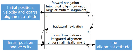
Figure 4.
Timing arrangement of the polar backtracking fine alignment.
The polar integrated fine alignment under a large azimuth misalignment is achieved using the algorithm in Section 2.3. The polar integrated alignment under a small misalignment is achieved using the algorithm in Section 2.4. The forward navigation algorithm, the backward data simulation generation strategy, and the backward navigation algorithm are shown below.
This paper establishes a transverse inertial forward navigation algorithm based on the transverse inertial mechanic’s arrangement proposed in Reference [14] and derives the transverse inertial backward navigation algorithm. The attitude, velocity, and position update algorithms for the transverse SINS are as follows [14]:
In the actual execution of the algorithm, it is necessary to discretize Equations (46)–(49) to obtain the corresponding recursive algorithm and define it as the forward navigation algorithm, which is shown below:
where
where represents the recursive cycle, , and is the inertial solving cycles. represents the rotation change of frame with respect to the reference frame, , from time to time , and represents the rotation change of frame with respect to the reference frame, , from time to time .
The backward navigation algorithm can be obtained by rearranging Equations (50)–(53) through a series of variable substitutions and algebraic manipulations.
Clearly, by comparing (50)–(53) and (55)–(58), it can be seen that to achieve backward navigation, it is only necessary to take the negative of the results of , , , and . Therefore, the specific method of simulating backward data using the stored data from the forward process is as follows:
Firstly, the stored data of the gyroscope and accelerometer in the forward process are reversed, and then the Earth’s rotation angular velocity, , gyroscope output angular rate, , and initial velocity for reverse navigation are negated to obtain the simulated reverse data.
In summary, the proposed backtracking fine alignment method consists of the following steps:
- Use Equations (50)–(53) and the algorithm in Section 2.3 to perform forward navigation and achieve the polar integrated fine alignment under the large misalignment;
- Utilize the data required for the backward navigation process generated through forward data simulation, and use the initial navigation parameters estimated for the forward navigation process, which consist of the attitude, velocity, and position at the final time, to perform backward navigation with Equations (55)–(58);
- Using the known initial position and velocity at the starting time for the forward navigation process, the attitude obtained from the backward navigation process at the final time is employed as the initial attitude for the forward navigation process. Equations (50)–(53) and the algorithm in Section 2.4 are then used to perform forward navigation and achieve a precise alignment of the small misalignment angle combination, resulting in the attitude matrix, , at the final time and completing the alignment of the dynamic base.
4. Experimental Results and Analysis
In this section, we carried out numerical experiments to evaluate the effectiveness of our algorithm. Limited by the geographical location of the authors’ country, which is far away from the Arctic, we conducted semi-physical experiments. The definite latitude and longitude determine the navigation systems’ ideal output, independent of the location of the carrier. Thus, the truth value generated by the trajectory generator and the sensor errors extracted from the SINS and DVL were synthesized to construct the semi-physical experimental data. The experiments were conducted to verify the performance of the inertial frame coarse alignment algorithm aided by the based on the transverse Earth model, the polar backtracking coarse alignment algorithm, and the polar backtracking fine alignment algorithm proposed in this paper.
4.1. Semi-Physical Experimental Conditions
The inertial measurement unit (IMU), composed of the three-axis gyroscope and accelerometer, provided the measured data of the SINS, as shown in Figure 5. The inertial measurement unit was installed on a high-precision turntable, as shown in Figure 6.
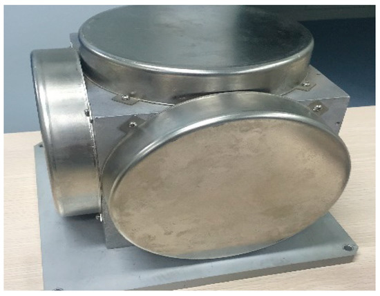
Figure 5.
Inertial measurement unit.
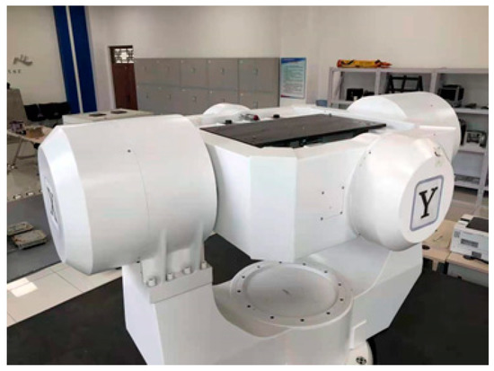
Figure 6.
High-precision three-axis turntable with the SINS.
The ideal output, and , can be inverted from the determined trajectory, and the IMU outputs the practical and . Thus, the measurement error is
After the subtraction, the sensor errors were as follows. The three-axis gyro constant drift was 6.3895 × 10⁻⁹ rad/s, −4.0947 × 10⁻⁹ rad/s, and −1.9605 × 10⁻⁹ rad/s. Its random drift was 3.917 × 10⁻⁶ rad/s, 3.264 × 10⁻⁶ rad/s, and 1.534 × 10⁻⁶ rad/s. The three-axis acceleration constant drift was 5.0024 × 10⁻⁶ m/s2, 2.7952 × 10⁻⁶ m/s2, and −7.2110 × 10⁻⁶ m/s2. Its random drift was 0.00161 m/s2, 0.001698 m/s2, and 0.0003726 m/s2.
The measurement error of the DVL-based velocity was extracted from the data resource of the sea trial near Dalian. The trial carried a ship-borne SINS/GNSS-integrated navigation system and the DVL. The SINS/GNSS-integrated navigation system output a velocity reference, , and the DVL output the measured velocity, . Thus, the measurement error of the DVL was:
The measurement error of the DVL is shown in Figure 7. Due to the interference by the actual environment, the noise contains large gross errors.
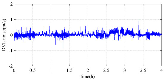
Figure 7.
The measurement error of the DVL.
To simulate the actual movement of the body in mid-latitude and polar regions, we designed a trajectory for the transverse Earth model, with the parameter settings as follows:
- (1)
- The navigation parameters in the mid-latitude region:
The initial position was (the initial position in the Earth model was ), the transverse eastward and northward errors were both 10 m, the initial attitude was , and the initial velocity was 5 m/s;
- (2)
- The navigation parameters in the polar region:
The initial position was (the initial position in the Earth model was ), the transverse eastward and northward errors were both 10 m, the initial attitude was , and the initial velocity was 5 m/s.
4.2. Performance Verification of the Inertial Frame Coarse Alignment Algorithm under the Transverse Earth Model
In order to validate the feasibility of the proposed inertial frame coarse alignment algorithm under the transverse Earth model in Section 2.2, this study employed the mid-latitude and polar motion scenarios designed in Section 4.1, and we conducted coarse alignment using both the traditional inertial frame coarse alignment algorithm [11] and the proposed algorithm under the transverse Earth model. The simulation duration was set to 600 s, and the experimental results are presented in Figure 8 and Figure 9, as well as in Table 2.
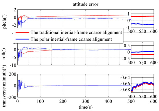
Figure 8.
Performance comparison of inertial frame coarse alignment algorithm in mid−latitude region.
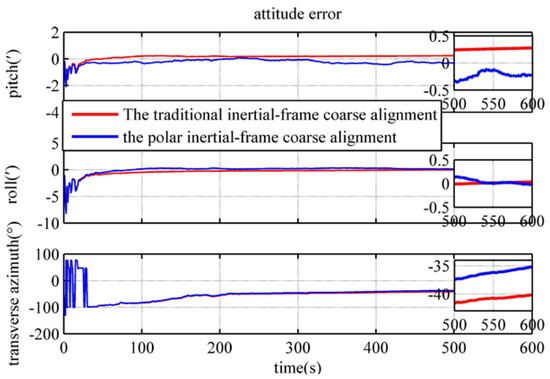
Figure 9.
Performance comparison of inertial frame coarse alignment algorithm in the polar region.
Table 2.
Coarse alignment results of different inertial frame coarse alignment algorithms with a simulation duration of 600 s.
Based on the analysis of Figure 8 and Figure 9 and Table 2, it can be observed that the alignment errors of both the traditional inertial frame coarse alignment algorithm and the proposed algorithm under the transverse Earth model gradually decrease with the increase in alignment time in different regions. In the mid-latitude region, the experimental results reveal that both algorithms have similar accuracy at 600 s, with attitude errors of less than 1′, and can achieve a coarse alignment of the moving base. Therefore, the feasibility of the proposed algorithm is verified in this region. In the polar region, the experimental results indicate that both algorithms have a horizontal attitude error of less than 1′ at 600 s, with transverse azimuth errors of −35.16° and −40.15°, respectively. The proposed algorithm under the transverse Earth model exhibits a higher azimuth accuracy, with an improvement of 12.43% compared to the traditional inertial frame coarse alignment algorithm. This improvement is attributed to the fact that the proposed algorithm eliminates the impact of longitude error amplification on the alignment in the polar region.
Additionally, a comparison of Figure 8 and Figure 9 reveals that the horizontal attitude error of both algorithms is not affected by increasing latitude, while the transverse alignment error increases with latitude. This is due to the fact that as the latitude increases, the earth vector and gravity vector tend to be aligned, reducing the coupling effect between the north direction and the azimuth loop, leading to a decrease in transverse alignment capability, while the horizontal attitude alignment capability is not affected. Therefore, in the polar region, although the transverse alignment error of the inertial coarse alignment algorithm under the transverse earth model is smaller than that of the traditional inertial frame coarse alignment algorithm, it still results in a large alignment error.
4.3. Performance Verification of the Polar Backtracking Coarse Alignment Algorithm
To verify the performance of the polar backtracking coarse alignment algorithm presented in Section 3.1, we utilized the polar motion scenario designed in Section 4.1 and performed coarse alignment using both the inertial frame coarse alignment algorithm under the transverse earth model and the polar backtracking coarse alignment algorithm. The simulation lasted for 180 s, and the experimental results are shown in Figure 10 and Table 3. It should be noted that since the backtracking coarse alignment algorithm does not affect the final velocity and position error of the moving base alignment, this section only presents a comparison of the attitude error between the two algorithms and analyzes the attitude accuracy and alignment time of the polar backtracking coarse alignment algorithm.
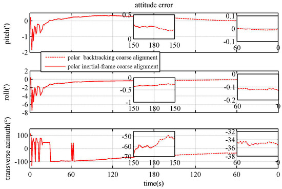
Figure 10.
Comparison of attitude errors between two algorithms.
Table 3.
Alignment results of two coarse alignment algorithms.
Based on the results presented in Figure 10 and Table 3, both algorithms achieved a horizontal attitude error of less than 1′ after 180 s of semi-physical simulation data. The transverse azimuth error for the inertial frame coarse alignment algorithm under the transverse Earth model was −59.86°, while that for the polar backtracking coarse alignment algorithm was −35.37°, indicating a 40.91% higher azimuth accuracy for the polar backtracking coarse alignment algorithm than that for the inertial frame coarse alignment algorithm under the transverse Earth model. The experimental results show that both algorithms have a small horizontal attitude error, which meets the alignment requirements. The polar backtracking coarse alignment algorithm has a smaller transverse azimuth error than the inertial frame coarse alignment algorithm under the transverse Earth model. This is mainly because the inertial frame coarse alignment algorithm under the transverse Earth model requires a longer time to complete the alignment in the polar region, and its alignment result cannot fully converge within 180 s, leading to a larger transverse azimuth error. However, the polar backtracking coarse alignment algorithm extends the alignment time, and its alignment result can further converge, resulting in a smaller transverse azimuth error.
Moreover, since the polar motion navigation parameters in Section 4.2 are consistent with those in Section 4.3, a comprehensive comparison of Table 2 and Table 3 shows that the transverse azimuth error of the inertial frame coarse alignment algorithm under the transverse earth model at 600 s is −35.16°. However, by utilizing semi-physical simulation data with a duration of 180 s, the polar backtracking coarse alignment algorithm yields a transverse azimuth error of −35.37°, which is similar to that of the former algorithm. Therefore, employing the polar backtracking coarse alignment algorithm can effectively save alignment time while the alignment accuracy is not compromised.
4.4. Performance Verification of the Polar Backtracking Fine Alignment Algorithm
According to reference [18], the polar integrated fine alignment under a large azimuth misalignment can complete the alignment in 600 s. To verify the performance of the polar backtracking fine alignment algorithm proposed in Section 3.2, we simulated the polar motion scenario designed in Section 4.1. Then, we compared the attitude, velocity, and position errors at the end of the alignment using the backtracking fine alignment algorithm and the integrated fine alignment under a large azimuth misalignment in Section 2.3 for 180 s and 600 s, respectively, after simulating for 180 s with the backtracking coarse alignment algorithm. The results are shown in Figure 11, Figure 12, Figure 13, Figure 14, Figure 15 and Figure 16 and Table 4. It should be noted that, according to the backtracking fine alignment steps in Section 3.2, the backtracking fine alignment algorithm will use the known initial velocity and position to correct the inertial velocity and position after backward navigation. Therefore, to obtain the velocity and position errors of the backtracking fine alignment algorithm, only the simulation results of Step 3 need to be presented, as shown in Figure 12 and Figure 13.
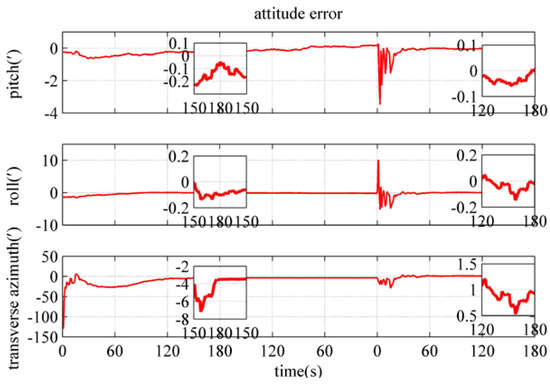
Figure 11.
The attitude error of the polar backtracking fine alignment algorithm.
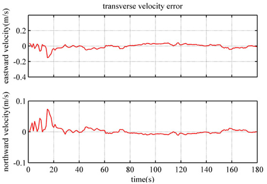
Figure 12.
The velocity error of the polar backtracking fine alignment algorithm.
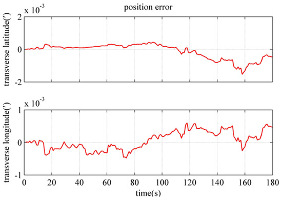
Figure 13.
The position error of the polar backtracking fine alignment algorithm.
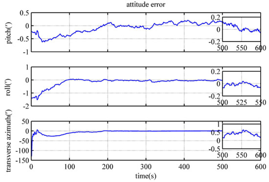
Figure 14.
The attitude error of the polar integrated fine alignment algorithm under large azimuth misalignment.
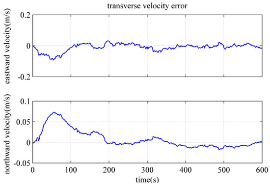
Figure 15.
The velocity error of the polar-integrated fine alignment algorithm under large azimuth misalignment.
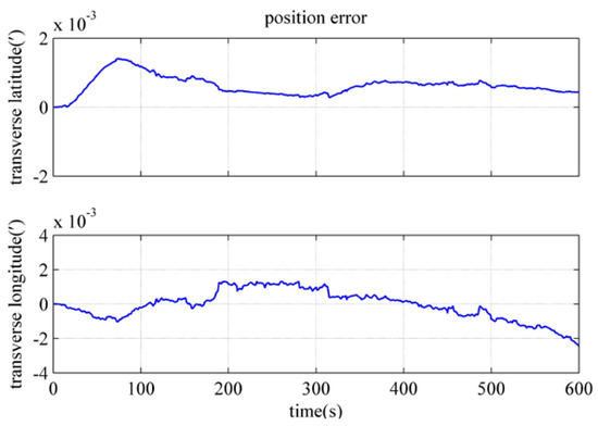
Figure 16.
The position error of the polar-integrated fine alignment algorithm under large azimuth misalignment.
Table 4.
Alignment results of two precise alignment algorithms.
According to Figure 11, Figure 12, Figure 13, Figure 14 and Figure 15 and Table 4, the polar integrated fine alignment under a large azimuth misalignment achieves a transverse attitude error of less than 1′ and a transverse azimuth error of −3.502′ at 180 s. The attitude errors for the polar backtracking fine alignment algorithm are also less than 1′. The transverse azimuth error is significantly improved by 73.59%. This is due to the fact that the alignment time is short, and the filtering of the polar-integrated fine alignment algorithm under a large azimuth misalignment has not fully converged yet. At 600 s, the polar-integrated fine alignment algorithm also achieves an attitude error of less than 1′, which meets the accuracy requirements of the alignment for the polar region. The difference in transverse velocity errors between the two algorithms is not significant, mainly because both algorithms can obtain the body velocity provided by the DVL. When the attitude error is small, the DVL velocity can be converted into transverse velocity with small errors and provided to the integrated alignment system. At both 180 s and 600 s, the attitude errors for both algorithms are relatively small, which results in similar transverse velocities. However, at 600 s, the position error of the polar-integrated fine alignment algorithm is larger than that of the integrated alignment algorithm under a large azimuth misalignment. This is because the observability of the position of the integrated alignment system is poor when only the body velocity is available for assistance, and the position error gradually accumulates as the alignment time increases. Overall, compared with the integrated alignment algorithm under a large azimuth misalignment, the polar backtracking fine alignment algorithm not only has smaller positioning errors but also requires less alignment time, which is 70% less than that of the integrated precision alignment algorithm under a large azimuth misalignment.
5. Conclusions
In this study, we proposed a polar moving base alignment method based on a backtracking scheme to achieve fast and high-precision alignment in the polar region. Firstly, a polar coarse alignment algorithm in the inertial frame under the transverse Earth model was designed to eliminate the effect of the alignment algorithm caused by longitude error amplification. Then, the polar coarse and fine alignment methods based on a backtracking scheme were designed, respectively. In the coarse alignment, the data storage scheme was optimized to reduce the computational burden. In the fine alignment, we derived the forward and backward navigation algorithms for the transverse SINS suitable for polar regions. We design a backtracking scheme that combines the alignment with a large azimuth misalignment and small misalignment, which ensures alignment accuracy and reduces the alignment time. The results of semi-physical simulation experiments show that, compared with previous methods, the coarse alignment algorithm in the inertial frame under the transverse Earth model increased the azimuth accuracy by 12.43%, the retrograde coarse alignment algorithm increased the azimuth accuracy by 40.91%, and the retrograde fine alignment method increased the azimuth accuracy by 73.59%. The algorithm proposed in this paper has a promising application prospect in the polar region.
Author Contributions
Conceptualization, J.L. and J.C. (Jianhua Cheng); methodology, J.L.; validation, J.L.; formal analysis, J.L.; writing—original draft preparation, J.L.; writing—review and editing, Y.W. and J.C. (Jing Cai). All authors have read and agreed to the published version of the manuscript.
Funding
This research was funded by the National Natural Science Foundation of China under Grant 62073093 and Grant 62003108, in part by the Science Fund for Distinguished Young Scholars of Heilongjiang Province under Grant JC2018019, and in part by the Basic Scientific Research Fund under Grant 3072020CFT0403.
Data Availability Statement
Not applicable.
Conflicts of Interest
The authors declare no conflict of interest.
References
- Berkman, P.A.; Vylegzhanin, A.N. Environmental Security in the Arctic Ocean; Springer: Berlin/Heidelberg, Germany, 2012. [Google Scholar]
- Cheng, J.; Liu, J.; Zhao, L. Survey on polar marine navigation and positioning system. Chin. J. Ship Res. 2021, 16, 16–29. [Google Scholar]
- Zhou, J.; Nie, X.; Lin, J. A novel laser doppler velocimeter and its integrated navigation system with strapdown inertial navigation. Opt. Laser Technol. 2014, 64, 319–323. [Google Scholar] [CrossRef]
- Yao, Y.; Xu, X.; Zhang, T.; Hu, G. An improved initial alignment method for sins/gps integration with vectors subtraction. IEEE Sens. J. 2021, 21, 18256–18262. [Google Scholar] [CrossRef]
- Liu, M.; Li, G.; Gao, Y. Improved polar inertial navigation algorithm based on pseudo INS mechanization. Aerosp. Sci. Technol. 2018, 77, 105–116. [Google Scholar] [CrossRef]
- Cai, J.; Cheng, J.; Zhong, S. An Innovative Polar Rapid Transfer Alignment Aided by Doppler Velocity Log For Marine Vessels. In Proceedings of the 2019 European Navigation Conference, Warsaw, Poland, 9–12 April 2019. [Google Scholar]
- Luo, L.; Huang, Y.; Zhang, Z.; Zhang, Y. A New Kalman Filter-Based In-Motion Initial Alignment Method for DVL-Aided Low-Cost SINS. IEEE Trans. Veh. Technol. 2021, 70, 331–343. [Google Scholar]
- Xu, X.; Guo, Z.; Yao, Y.; Zhang, T. Robust Initial Alignment for SINS/DVL Based on Reconstructed Observation Vectors. IEEE/ASME Trans. Mechatron. 2020, 25, 1659–1667. [Google Scholar] [CrossRef]
- Pei, F.; Yang, S.; Yin, S. In-Motion Initial Alignment Using State-Dependent Extended Kalman Filter for Strapdown Inertial Navigation System. IEEE Trans. Instrum. Meas. 2021, 70, 1–12. [Google Scholar] [CrossRef]
- Zhang, Q.; Li, S.; Xu, Z. Velocity-based optimization-based alignment (VBOBA) of low-end MEMS IMU/GNSS for low dynamic applications. IEEE Sens. J. 2020, 20, 5527–5539. [Google Scholar] [CrossRef]
- Xu, J.; He, H.; Qin, F. A novel autonomous initial alignment method for strapdown inertial navigation system. IEEE Trans. Instrum. Meas 2017, 66, 2274–2282. [Google Scholar] [CrossRef]
- Ouyang, W.; Wu, Y. Optimization-based strapdown attitude alignment for high-accuracy systems: Covariance analysis with applications. IEEE Trans. Aerosp. Electron. Syst. 2022, 58, 4053–4069. [Google Scholar] [CrossRef]
- Li, Y.; Liu, M.; Gong, J. Double-velocity inertial-frame alignment algorithm with pseudo INS modeling in polar regions. J. Syst. Eng. Electron. 2022, 44, 1677–1684. [Google Scholar]
- Yao, Y.; Xu, X.; Li, Y.; Liu, Y.; Sun, J. Transverse navigation under the ellipsoidal earth model and its performance in both polar and non-polar areas. J. Navig. 2016, 69, 335–352. [Google Scholar] [CrossRef]
- Cai, J.; Cheng, J.; Liu, J.; Wang, Z.; Xu, Y. A polar rapid transfer alignment assisted by the improved polarized-light navigation. IEEE Sens. J. 2022, 22, 2508–2517. [Google Scholar] [CrossRef]
- Wu, Y.; He, C.; Liu, G. On inertial navigation and attitude initialization in polar areas. Satell. Navigat 2020, 1, 4. [Google Scholar]
- Liu, J.; Zhao, L.; Qi, B.; Cheng, J.; Cai, J. A new polar integrated alignment algorithm with the aids of DVL and the improved polarized-light navigation. In Proceedings of the Name of the 2022 5th International Symposium on Autonomous Systems. (ISAS), Hangzhou, China, 8–10 April 2022. [Google Scholar]
- Yan, Z.; Wang, L.; Wang, T.; Zhang, H.; Yang, Z. Polar transversal initial alignment algorithm for UUV with a large misalignment angle. Sensors 2018, 18, 3231. [Google Scholar] [CrossRef]
- Cheng, J.; Liu, J.; Cai, J.; Xu, Y. A Polar Integrated Alignment Assisted by DVL Under Large Azimuth Misalignment. IEEE Sens. J. 2023, 23, 5962–5973. [Google Scholar] [CrossRef]
- Wen, Z.; Yang, G.; Cai, Q. Odometer aided SINS in-motion alignment method based on backtracking scheme for large misalignment angles. IEEE Access 2020, 8, 7937–7948. [Google Scholar] [CrossRef]
- Sun, Y.; Yang, G.; Cai, Q. A robust in-motion attitude alignment method for odometer-aided strapdown inertial navigation system. Rev. Sci. Instrum. 2020, 91, 125006. [Google Scholar] [CrossRef]
- Wang, D.S.; He, G.Y.; Jiang, X.H. In-motion Alignment Scheme Based on Reverse Kalman Filter. J. Chin. Inertial Technol. 2020, 28, 721–728. [Google Scholar]
- Lin, Y.; Miao, L.; Zhou, Z. A high-accuracy initial alignment method based on backtracking process for strapdown inertial navigation system. Measurement 2022, 201, 111712. [Google Scholar] [CrossRef]
- Wahba, G. A least squares estimate of satellite attitude. SIAM Rev. 1965, 7, 409. [Google Scholar] [CrossRef]
- Yan, G.; Chen, R.; Guo, K. Equivalence analysis between SVD and QUEST for multi-vector attitude determination. J. Chin. Inertial Technol. 2019, 27, 568–572. [Google Scholar]


Disclaimer/Publisher’s Note: The statements, opinions and data contained in all publications are solely those of the individual author(s) and contributor(s) and not of MDPI and/or the editor(s). MDPI and/or the editor(s) disclaim responsibility for any injury to people or property resulting from any ideas, methods, instructions or products referred to in the content. |
© 2023 by the authors. Licensee MDPI, Basel, Switzerland. This article is an open access article distributed under the terms and conditions of the Creative Commons Attribution (CC BY) license (https://creativecommons.org/licenses/by/4.0/).