Abstract
Detecting defects in power transmission lines through unmanned aerial inspection images is crucial for evaluating the operational status of outdoor transmission equipment. This paper presents a defect recognition method called EDF-YOLOv5, which is based on the YOLOv5s, to enhance detection accuracy. Firstly, the EN-SPPFCSPC module is designed to improve the algorithm’s ability to extract information, thereby enhancing the detection performance for small target defects. Secondly, the algorithm incorporates a high-level semantic feature information extraction network, DCNv3C3, which improves its ability to generalize to defects of different shapes. Lastly, a new bounding box loss function, Focal-CIoU, is introduced to enhance the contribution of high-quality samples during training. The experimental results demonstrate that the enhanced algorithm achieves a 2.3% increase in mean average precision (mAP@.5) for power transmission line defect detection, a 0.9% improvement in F1-score, and operates at a detection speed of 117 frames per second. These findings highlight the superior performance of EDF-YOLOv5 in detecting power transmission line defects.
1. Introduction
The electric power industry is rapidly developing due to the gradual rise in electricity demand, which brings substantial challenges in maintaining the existing transmission lines [1]. Furthermore, transmission lines span extensive areas and endure prolonged exposure to the elements, rendering them susceptible to various transmission defects, including insulator damage, insulator pollution flashovers, and bird nest attachments [2]. These issues can be exacerbated by intricate external environmental conditions, posing significant threats to the regular operation of transmission lines [3,4,5].
To prevent faults, the initial approach involved manual patrolling to inspect power transmission line defects. Nevertheless, these conventional manual patrolling methods are not only time-consuming and labor-intensive but also introduce specific risks to the patrolling personnel [6,7].
With the advancement of society and technology, unmanned aerial vehicles (UAVs), commonly referred to as drones, have gained widespread application in the patrol inspection of transmission lines [8]. This innovative inspection method utilizes target detection algorithms to identify defects in images captured by drones, representing a more efficient and technologically advanced approach to detecting and maintaining transmission lines [9,10].
However, it also presents new challenges. For instance, the varied shooting angles of drones and the complex backgrounds of captured targets can all influence the detection accuracy of target detection algorithms [11]. Therefore, the urgent issue at hand is how to enhance the detection accuracy of target detection algorithms for images of power transmission line defects captured by drones [12].
Currently, mainstream target detection algorithms are categorized into two main classes based on whether they involve a separate candidate box generation stage: two-stage target detection algorithms and one-stage target detection algorithms [13]. Prominent two-stage target detection algorithms include Fast R-CNN (Fast Region-Convolutional Neural Network) [14], Faster R-CNN (Faster Region-Convolutional Neural Network) [15], and the like. Two-stage object detection algorithms have demonstrated excellent detection performance in practical applications, but their complexity results in slower detection speeds, limiting their real-time applicability [16].
Mainstream one-stage target detection algorithms include the YOLO (You Only Look Once) series and the SSD (Single Shot MultiBox Detector) series algorithms [17]. One-stage target detection algorithms eliminate the separate stage for candidate box generation, leading to more streamlined models. In this series of algorithms, feature extraction, candidate box regression, and classification all take place within the same convolutional network, resulting in faster detection speeds compared to their two-stage counterparts [18,19].
In recent years, the field of transmission line defect detection through drone patrol inspections has garnered significant interest. Given the small size and fast detection speed of YOLO series algorithms, they have found wide application in this domain. However, YOLO series algorithms have been associated with lower detection accuracy in transmission line defect detection. To address this issue, several scholars have proposed improvements. Hu et al. [20] introduced a BiFPN module for feature fusion, effectively enhancing the defect detection capabilities of the YOLOv5s algorithm. Additionally, to overcome the challenge of detecting small defects on insulators, they integrated an SPD module. Han et al. [21] introduced SA-Net and Multi-head output to improve YOLOv4’s ability to recognize small targets in insulator defects. Bao et al. [22] improved YOLOv5 by adding a coordinate attention module, allowing it to pay more attention to the features of vibration dampers and insulators. Qiu et al. [23] optimized YOLOv4 using the MobileNet lightweight convolutional neural network to enhance the algorithm’s detection speed for defects on transmission lines. Despite the numerous improvements made in YOLO series algorithms in recent years, there have been relatively few enhancements specifically targeting the YOLOv5s algorithm in the field of transmission line defect detection. Therefore, to date, there is still significant room for improvement in the accuracy of YOLOv5s algorithm for detecting transmission line defects, particularly for small target defects and defects with substantial shape variations.
To address the issues mentioned above, we have proposed an improved version of YOLOv5 for detecting defects in power transmission lines. The main contributions of this paper are as follows:
- We have designed a module with enhanced feature extraction capabilities, referred to as EN-SPPFCSPC. This module outperforms Spatial Pyramid Pooling-Fast and Fully Connected Spatial Pyramid Convolution (SPPFCSPC), providing higher detection accuracy while maintaining a lower parameter count. EN-SPPFCSPC effectively leverages feature information, reducing the loss of detailed information, and significantly enhancing detection accuracy.
- We have introduced a high-level semantic information extraction module, DCNv3C3, with stronger adaptive capabilities. This module is employed to replace the C3 module in the YOLOv5s algorithm’s neck. This improvement effectively boosts the algorithm’s generalization ability, enabling it to perform better in various scenarios.
- To expedite model convergence and enhance detection accuracy, we have proposed the Focal-CIoU loss function. This novel loss function aims to augment the gradient contribution of high-quality samples during the training process.
2. Methods
2.1. Network Architecture
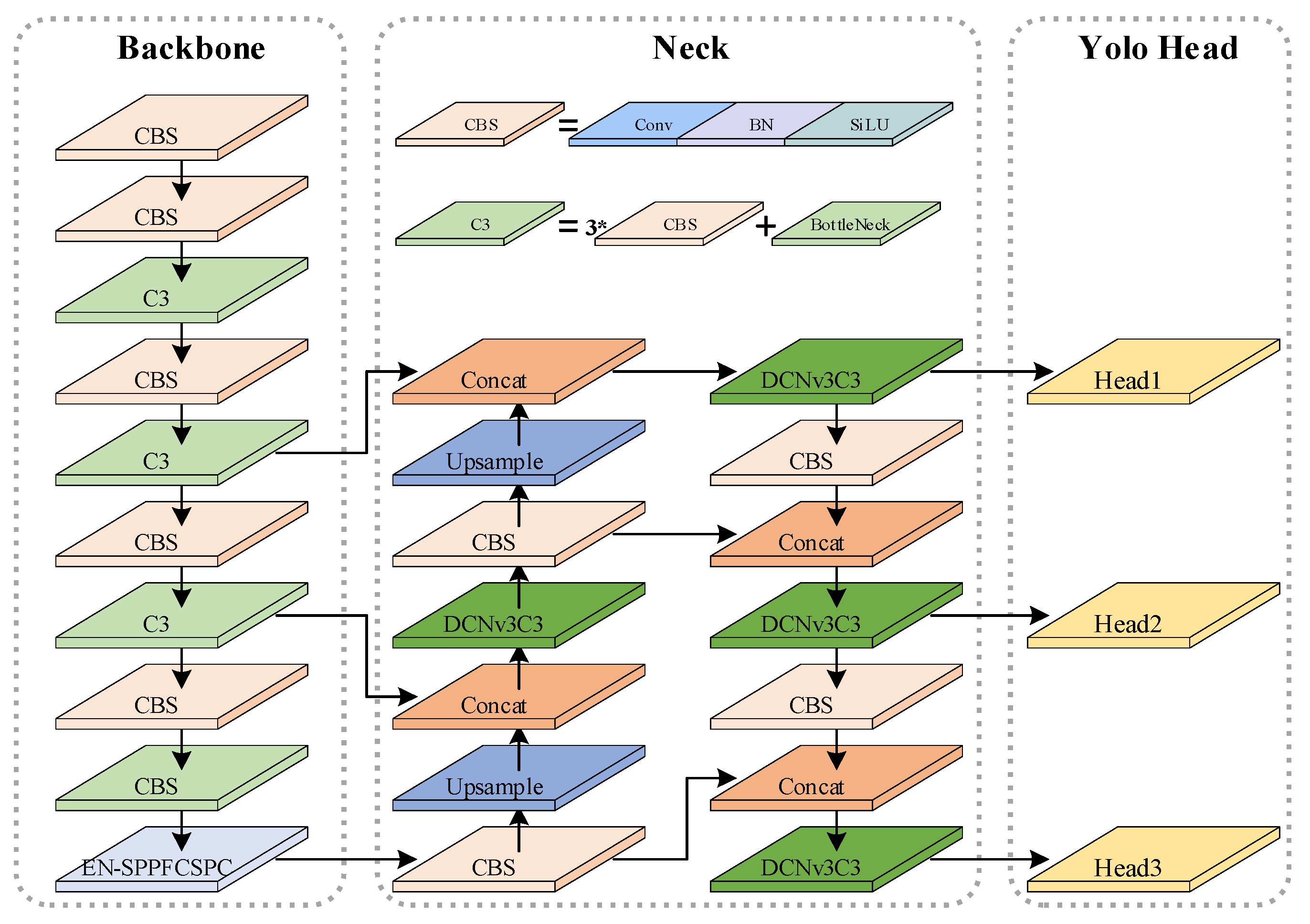
The YOLOv5 algorithm was developed by Glenn Jocher and his team in 2020. This algorithm effectively balances detection speed and accuracy, making it widely applicable in the field of object detection [24]. The YOLOv5 algorithm comprises three main components: the backbone, the neck, and the detection head [25]. Input images first undergo feature extraction in the backbone, generating three useful feature layers that are then passed to the neck network. The neck module performs feature fusion on the incoming feature layers. The top-down part of the neck network achieves feature fusion across different scales through up-sampling and fusion with coarser-grained feature maps. Subsequently, the bottom-up part mainly employs convolutional layers to fuse features across different scales. Finally, the feature maps from both the top-down and bottom-up parts are combined to obtain the ultimate feature map [26]. The detection head serves as the classifier and regressor of the YOLOv5 model, assessing the features from the neck network to detect target objects [27]. In this paper, the YOLOv5s algorithm is enhanced to produce EDF- YOLOv5, which offers increased accuracy in detecting defects on transmission lines, as shown in Figure 1. Firstly, in the YOLOv5s backbone network, we introduce the EN-SPPFCSPC module to replace the Spatial Pyramid Pooling-Fast module (SPPF). The EN-SPPFCSPC comprehensively utilizes feature information, preventing the significant loss of detailed information, and thereby enhancing the algorithm’s capability to detect small target defects in power transmission lines. Secondly, we replace the C3 modules in the algorithm’s neck network section with DCNv3C3. This modification effectively enhances the algorithm’s ability to generalize across various shapes of power transmission line defects. Lastly, we introduce the Focal-CIoU loss function, replacing CIoU. This change enhances the gradient contributions of high-quality samples during the training process, effectively improving the algorithm’s convergence speed and detection accuracy.
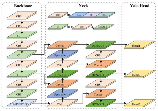
Figure 1.
EDF-YOLOv5 structure diagram.
2.2. EN-SPPFCSPC Module
In this paper, we are inspired by the SPPFCSPC structure [28] and introduce EN-SPPFCSPC, which has improved feature extraction capabilities, effectively preventing the loss of detailed information in defective targets. The advantages of the EN-SPPFCSPC module primarily stem from two key improvements. Firstly, we employ three -sized SoftPool [29] sub-regions as a replacement for the max-pooling in SPPFCSPC. This substitution effectively mitigates the substantial loss of fine-grained details. SoftPool, applied to the input feature layer, activates feature points using a softmax-weighted approach within the pooling region. It then computes the weighted sum of all activated points within the pooling area, ultimately yielding the activation output of the pooling neighborhood. The principle of SoftPool is depicted in Figure 2, where, assuming a pooling kernel size of , we calculated the weight values,, for each pixel point, , within the feature region, R. If the pixel value of each point is , the activation weight is determined using Equation (1).
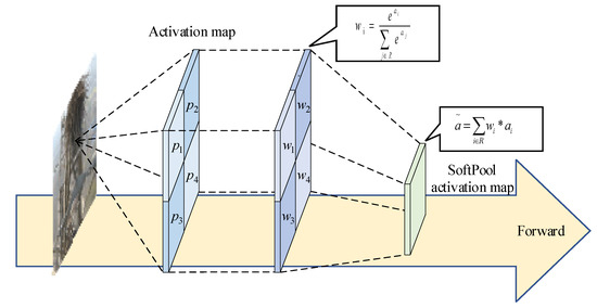
Figure 2.
SoftPool schematic diagram.
Subsequently, the weights are assigned to the respective pixel points and subjected to weighted summation, yielding the SoftPool output result, , as shown in Equation (2).
SoftPool comprehensively considers every feature point within the pooling neighborhood, reducing information loss while preserving the overall receptive field. Moreover, each input feature receives a gradient, contributing to enhanced training effectiveness.
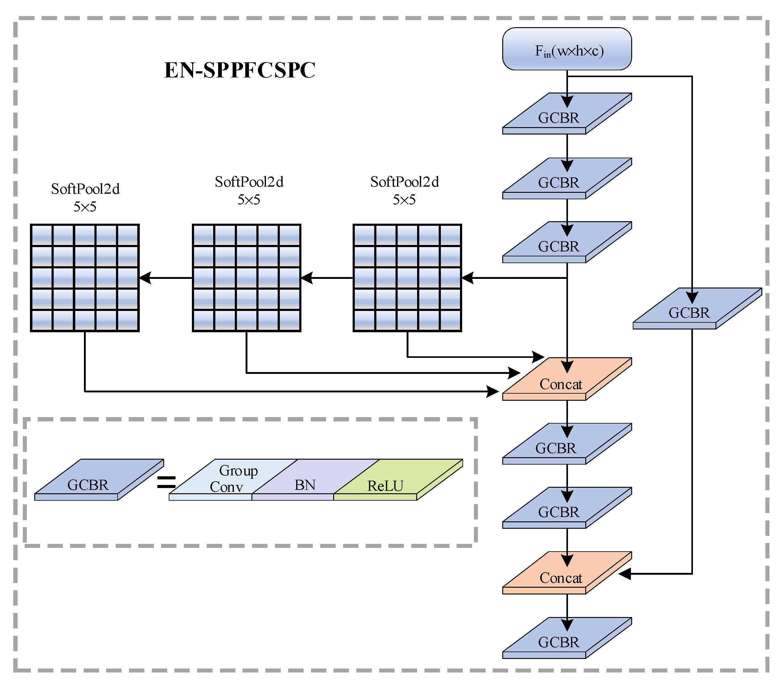
Furthermore, to effectively reduce the number of parameters, EN-SPPFCSPC introduces a multi-group mechanism concept, employing group convolution in place of a conventional convolution. For the input feature maps, it is divided into four groups along the channel dimension; convolution operations are then performed on each of these groups. The EN-SPPFCSPC structure is illustrated in Figure 3. The input feature map undergoes feature extraction through two branches: one branch contains only a GCBR module, which is composed of grouped convolution, batch normalization, and the Relu activation function. The GCBR module in this branch utilizes a convolutional kernel for grouped convolution with a group number of 4, effectively reducing the number of parameters and facilitating inter-channel information interaction. The other branch consists of three serial SoftPool operations with convolutional kernels of size , along with multiple GCBR modules. In this branch, the feature map sequentially undergoes three SoftPool operations, followed by concatenation of the outputs from the three SoftPools and the output from the third GCBR along the channel dimension. This approach effectively controls the parameter count and maximizes the utilization of fine-grained feature information in the feature map. The EN-SPPFCSPC module, with its ability to fully integrate feature information, significantly enhances the algorithm’s capability to detect small defective targets.
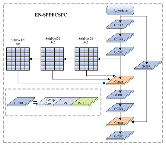
Figure 3.
EN-SPPFCSPC structure diagram.
2.3. DCNv3C3 Module
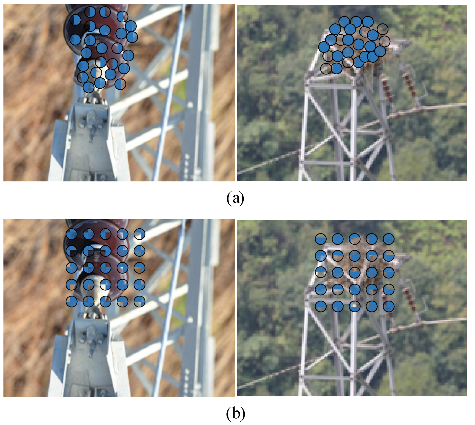
YOLOv5s employs fixed geometric structures for its convolution kernels, inherently limiting its ability to model geometric transformations. Therefore, in this paper, we combine the C3 module with Deformable Convolution v3 (DCNv3) [30] to propose the DCNv3C3 module, which exhibits an enhanced adaptability to cope with changes in the shape of the target object. DCNv3 can adjust the sampling positions of convolution by position-offset maps, allowing the sampling points to better focus on the target objects. Simultaneously, it adjusts the weights of sampling points through the modulation maps. Therefore, compared to regular convolution, DCNv3 exhibits superior generalization capabilities, enabling it to adaptively locate and activate target units. A visual comparison of the sampling effects between regular convolution and DCNv3 is shown in Figure 4.

Figure 4.
(a) Illustration of the sampling effect of DCNv3. (b) Illustration of the sampling effect of ordinary convolution.
Normal convolution employs fixed convolution kernels, D, to sample the input feature map . The final output is obtained by weighting the convolution kernel’s weights with the pixel values at the sampling points. For example, with a 3 × 3 convolution kernel, considering the center position as the reference, each sampling point’s relative position coordinates can be represented as . The mathematical expression for normal convolution is provided in Equation (3):
In the equation, represents the sampled output of the convolution kernel, represents the projection weight of the sampling point of the convolution kernel, is the center position of the convolution kernel, and represents the pixel value of the input feature map at the corresponding sampling point location.
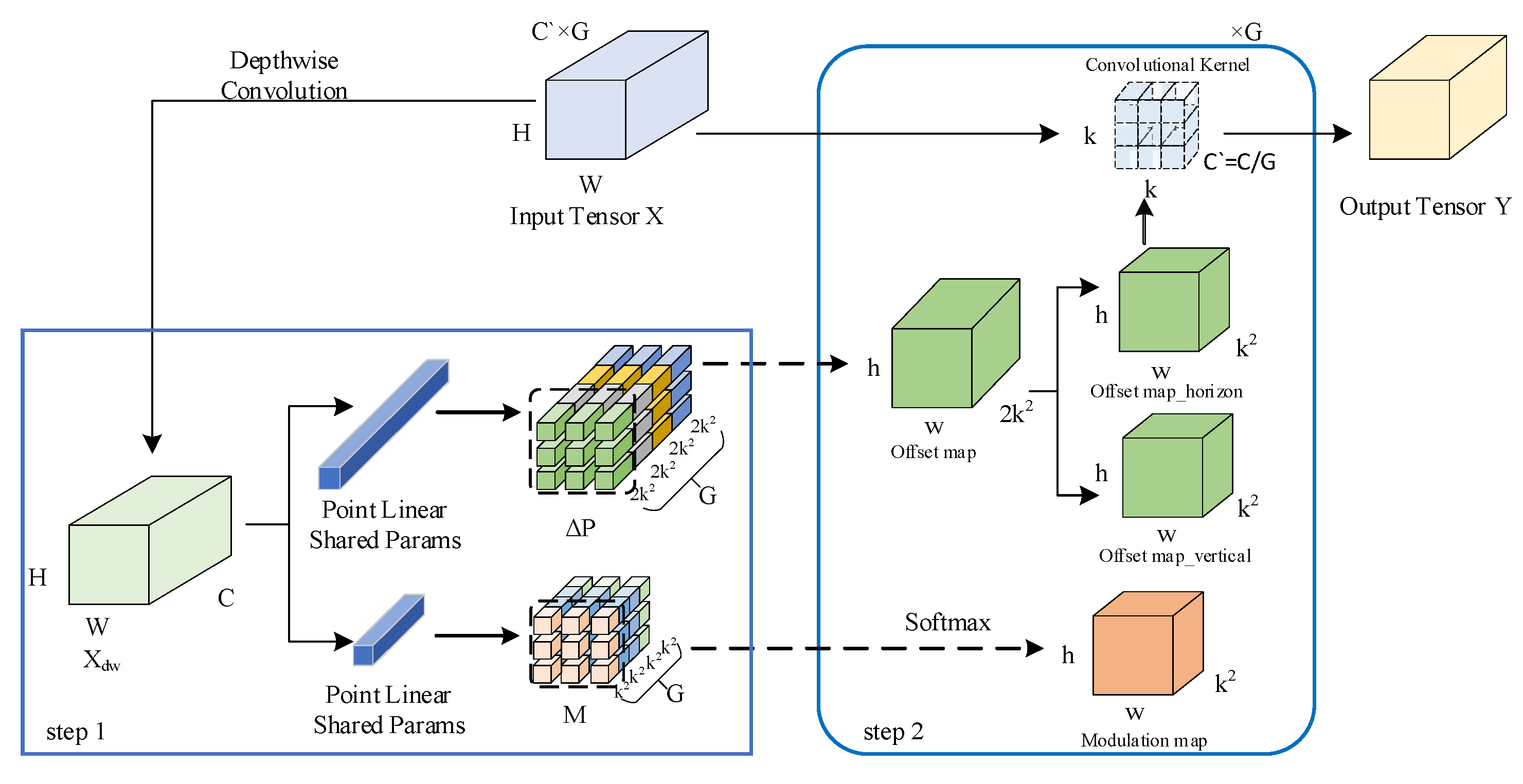
DCNv3 is depicted in Figure 5. Assuming that means the kernel size, the implementation of DCNv3 can be divided into two main steps. The first step involves conducting depth-wise and point-wise inferences on the input feature map , resulting in the generation of position-offset maps and modulation maps , where and represents the number of groups. In the second step, and M play flexible roles in the feature extraction procedure by focusing on the sampling object and modulating the weights, respectively. More detailed explanations with formulas are described in the following.
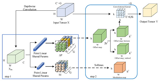
Figure 5.
DCNv3 schematic diagram.
In the first step, the depth-wise direction inference, as indicated by Equation (4), and the channel-wise operation, are applied to the input , which then results in :
where DConv(·) is the depth-wise convolution and converts channel dimensions to the last dimension. BN and GELU mean the normalization and activation function, respectively.
And the point-wise direction inference, as illustrated by Equations (5) and (6), a fully connected approach is employed to enable the sharing of projection weights among sampling points, ultimately computing bias offsets and modulation factors.
where denotes the shared linear layer applied to each sampling point. Note that M passes through a softmax function and is therefore stable in the dimension.
In the second step, grouping convolution operations are applied to the input, , during the convolution operation for each group; the adjustment of sampling points of the conventional convolution kernel is accomplished using position-offset and modulation factors. This adjustment aims to better focus the sampling points on the target features. The output for any pixel of the input feature map is expressed as per Equation (7). DCNv3 not only exhibits enhanced geometric transformation capabilities but also, through the application of grouped convolution, segregates the spatial aggregation process into G groups. This effectively controls the parameter count and introduces diverse spatial aggregation patterns to the sampling process, thereby providing stronger feature information for downstream tasks.
In the equation, represents the number of groups, represents the group, represents the projection weight for the sampling position of the convolution kernel used for sampling in the group, and represents the modulation factor of the sampling point in the group. represents the position-offset of the sampling point in the g-th group.
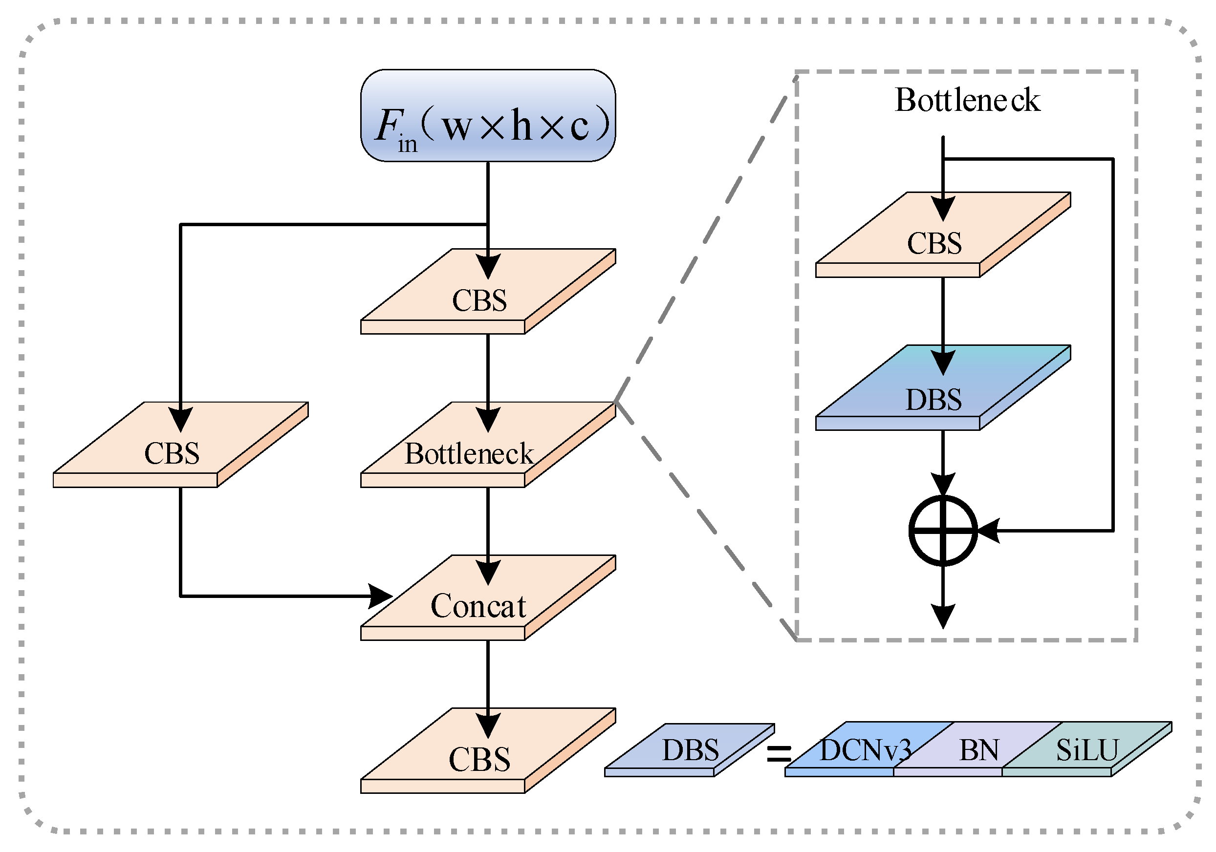
The structure of DCNv3C3 is illustrated in Figure 6, where DCNv3 is introduced into the C3 module. In the original C3 module, the BottleNeck part consists of two CSB structures and one residual connection. In the improved version, one of the CBS structures is optimized into a DBS structure which employs the more versatile DCNv3 in place of the normal convolution for feature sampling. The DCNv3C3 module requires setting the convolution group number for the DCNv3 operator based on the actual situation. In this paper, the parameters were set as follows according to the different numbers of input feature map channels: .

Figure 6.
DCNv3C3 structure diagram.
2.4. Focal-CIoU Loss Function
In the YOLOv5 algorithm, the default choice for bounding box regression loss is the CIoU loss function, as shown in Equations (8)–(10). This loss function takes into account three factors: the overlap area between the predicted and true bounding boxes, the centroid distance, and the aspect ratio. However, it overlooks the issue of imbalance between low-quality and high-quality samples. Low-quality samples refer to predicted boxes with minimal overlap with the target box. These anchor boxes result in larger regression errors and have a negative impact on training.
In Equations (8) and (10), represents the Euclidean distance between the predicted box and the true box’s center point, represents the diagonal length of the minimum closed bounding region of the two bounding boxes, and are the width and height of the predicted box, respectively, and and are the width and height of the true box, respectively.
To enhance the contribution of high-quality samples during training, this study drew inspiration from the Focal-EIoU loss function [31] and combined the ideas of the CIOU loss function and the Focal loss function, proposing the Focal-CIoU loss function. The Focal-CIoU loss function assigns weights to training samples based on IOU and the γ parameter, giving higher weights to high-quality samples. This reduces the contribution of low-quality samples in bounding box regression, allowing the algorithm to focus more on high-quality samples during training, which helps improve regression accuracy. The Focal-CIoU loss function is defined as follows in Equation (11):
where is a parameter used to control the degree of suppression of outliers. In this study, the parameter setting method from Focal-EIoU was adopted, with taking a value of 0.5.
3. Experimentation and Results Analysis
3.1. Experimental Conditions
This experiment was conducted on a Linux system, with an Intel Core i7-8700 CPU, NVIDIA Titan Xp GPU with 12 GB of memory, using CUDA 11.6 as the software environment, and PyTorch 1.12.1 as the deep learning framework. The Python version used was 3.8.8.
In this experiment, a total of 3985 aerial photographs of transmission line defects were used, of which 2845 were collected by the research team. The UAV model used for this collected dataset was the MAVIC PRO 2 with 12 megapixels, a range of 10 km, and a maximum flight altitude of 5000 m. The remaining 1140 aerial photos are from the web. The labeling process was carried out using “labelimg”, and the labeling format adhered to the PASCAL VOC standard. The annotation information for the dataset was uniformly saved in XML format. To enhance model training, efforts were made to ensure that the annotated bounding boxes closely matched the annotated objects.
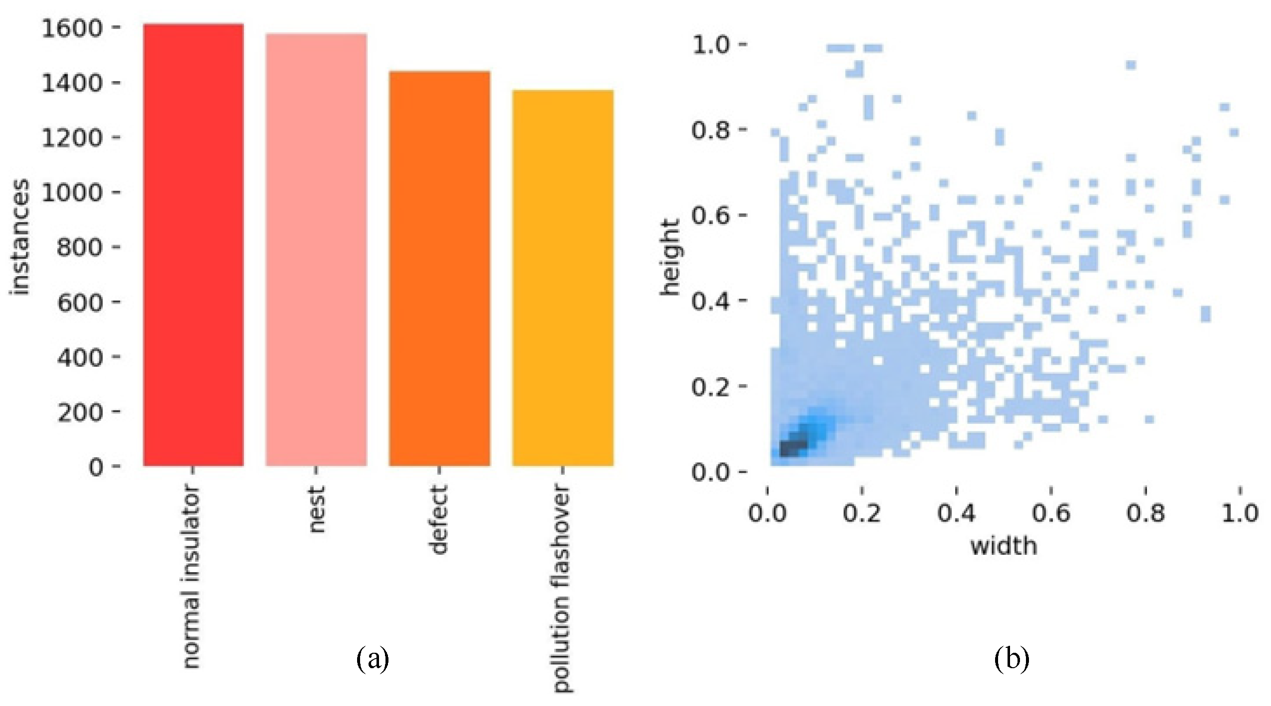
There were four target categories in total: Nest (for tower bird’s nest attachments), Defect (for insulator damage defects), Normal Insulator (for normal insulators), and Pollution Flashover (for insulator pollution flashover defects). The dataset was divided into training, testing, and validation sets in an 8:1:1 ratio. The distribution of sample labels in the dataset can be seen in Figure 7, and the transmission line defects are described in Table 1.

Figure 7.
(a) Distribution of label quantities in the dataset. (b) Distribution of label sizes.

Table 1.
Introduction of transmission line defects.
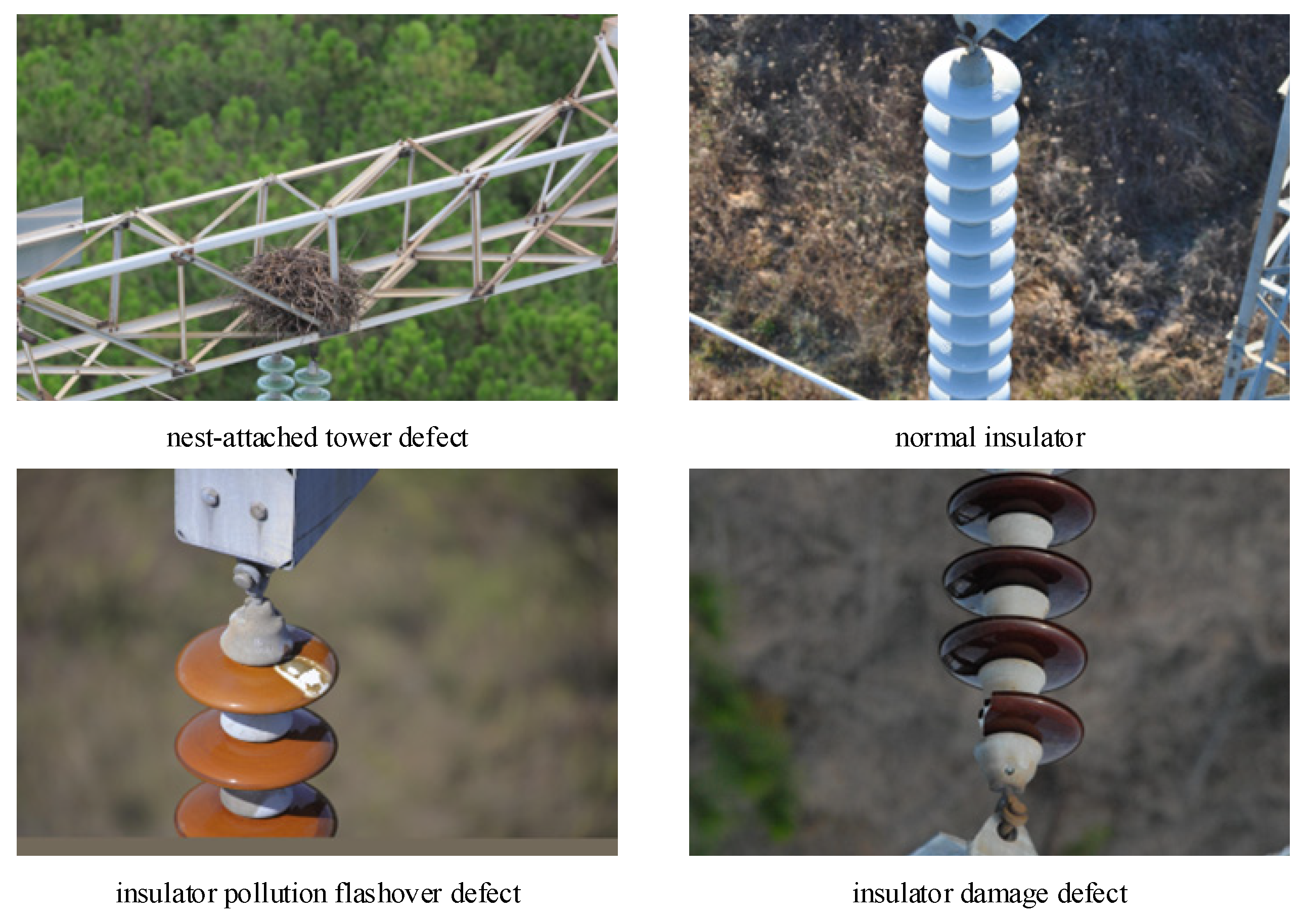
Aerial images depicting transmission line defects are shown in Figure 8.
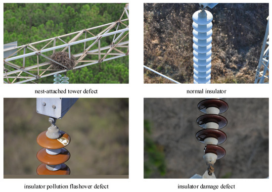
Figure 8.
Example images of the dataset.
3.2. Experimental Evaluation Indicators
The evaluation metrics involved in this experiment primarily include mean average precision (mAP), recall rate (R), precision (P), parameter count, frames per second (FPS), and F1-score. The calculation formulas are as follows (12)–(15).
TP represents the true positive samples in the detection results, FN represents the false negative samples in the detection results, and FP represents the false positive samples in the detection results. mAP is the mean average precision for all categories and the F1-score is a comprehensive metric that simultaneously considers precision and recall to evaluate the algorithm’s performance on positive and negative samples.
3.3. Comparison of Different Loss Functions in Experiments
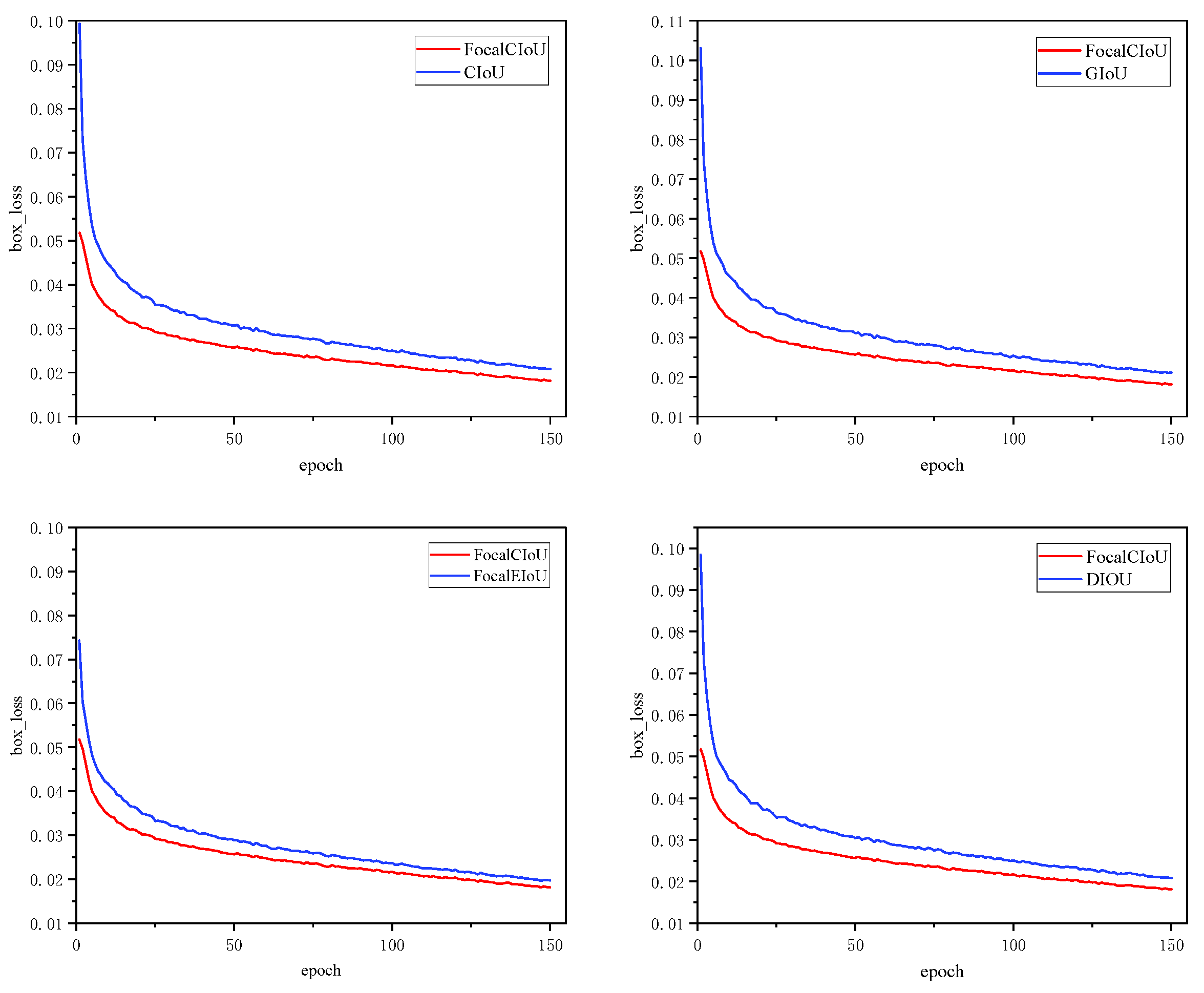
To validate the effectiveness of the Focal-CIoU loss function, this study conducted comparative experiments using the CIoU loss function, GIoU loss function, Focal-EIoU [31] loss function, and DIoU loss function. The experimental results are shown in Figure 9 and Table 2.
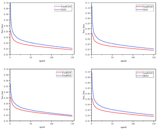
Figure 9.
Loss function experimental results comparison diagram.
Table 2.
Detection accuracy of different loss functions at mAP50.
Analyzing the results in conjunction with Figure 9 and Table 2, the following conclusions can be drawn. The Focal-CIoU loss function performs remarkably well during training, consistently showing lower initial loss values compared to the other four loss functions, and it converges quickly, reaching the lowest loss values below 0.02. Additionally, when YOLOv5s utilizes the Focal-CIoU loss function as the bounding box regression loss, it results in a 1.5% improvement in mAP@0.5. In summary, the Focal-CIoU loss function exhibits the best performance in this comparative experiment. This loss function enhances the gradient contribution of high-quality samples during training, making the model more robust and freer from overfitting issues.
3.4. Comparison of Different Spatial Pyramid Pooling Modules in Experiments
To validate the effectiveness of the EN-SPPFCSPC module, this section conducts comparative experiments using the SPPF module, the SPPFCSPC module, and the EN-SPPFCSPC module, respectively. The experimental results are shown in Table 3.
Table 3.
Comparison of experimental results using different spatial pyramid pooling modules.
From Table 3, it can be observed that the EN-SPPFCSPC model exhibited a favorable performance in this comparative experiment. With a parameter count similar to the SPPF module, the final mAP@0.5 value improved by 0.9%. Furthermore, compared to SPPFCSPC, the EN-SPPFCSPC module significantly reduced the parameter count while improving accuracy, achieving a lightweight effect. It is evident that the EN-SPPFCSPC module effectively utilized comprehensive information from feature maps, addressing the issue of the substantial loss of fine details in the YOLOv5s algorithm’s spatial pyramid pooling module. The standard for real-time object detection typically requires algorithms to process a certain number of frames per second (FPS). This criterion may vary depending on the application scenario, but, generally, the requirement for real-time object detection is around 30 FPS. According to this standard, the improved YOLOv5s algorithm with the SPPFCSPC enhancement performs exceptionally well on this dataset and meets the speed requirements for real-time detection.
3.5. Experimental Comparison of DCNv3C3 Module at Different Usage Positions
To verify the impact of DCNv3C3 on the detection accuracy of the YOLOv5s algorithm and to find the optimal placement of this module in the algorithm, this study conducted comparative experiments using three scenarios: the unmodified YOLOv5s algorithm, the use of the DCNv3C3 module in the backbone of the YOLOv5s algorithm, and the use of the DCNv3C3 module in the neck of the YOLOv5s algorithm. The experimental results are shown in Table 4.
Table 4.
Experimental comparison of DCNv3C3 module usage at different positions.
From Table 4, it can be observed that optimizing C3 in the Backbone of DCNv3C3 results in a slight improvement in average detection accuracy while reducing the parameter count. Specifically, mAP@0.5 improved by 0.6%, but the detection speed decreased by 37.8 frames per second, and there was a slight decrease in F1 score. On the other hand, optimizing C3 in the Neck to DCNv3C3 resulted in the most significant optimization effect for the algorithm. mAP@0.5 improved by 1.2%, F1 score increased significantly, and the model’s detection speed only slightly decreased. In summary, the DCNv3C3 module effectively enhances the YOLOv5s algorithm’s capability to detect transmission line defects.
3.6. Ablation Experiment
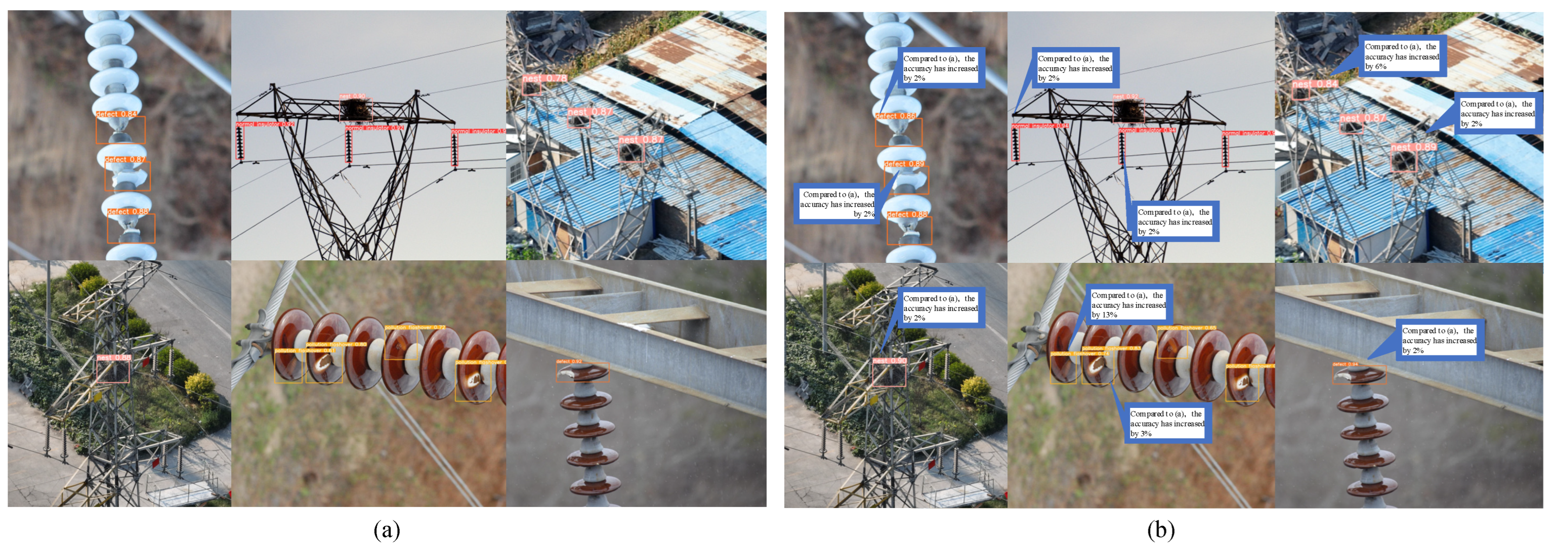
This paper proposes three improvements to the YOLOv5s algorithm. In order to explore the impact of these different improvements on the algorithm’s detection accuracy, ablation experiments were conducted. The experimental results are shown in Table 5, where √ indicates the usage of this module, where M0 represents the unimproved YOLOv5s algorithm, M1 represents the use of EN-SPPFCSPC as the algorithm’s spatial pyramid pooling module, M2 represents the optimization of the C3 module in the algorithm’s neck to the DCNv3C3 module, M3 represents the use of the Focal-CIoU loss function as the algorithm’s bounding box regression loss, M4 represents the simultaneous use of the EN-SPPFCSPC and DCNv3C3 modules for algorithm improvement, M5 represents the simultaneous use of the DCNv3C3 module and Focal-CIoU loss function for algorithm improvement, and M6 represents the simultaneous use of the EN-SPPFCSPC module and Focal-CIoU loss function for algorithm improvement. “Ours” represents the EDF-YOLOv5 obtained by simultaneously using all three of the above-mentioned improvements to enhance the algorithm. We randomly selected test data and performed detection using the YOLOv5s algorithm and an improved algorithm called EDF-YOLOv5. The detection results are shown in Figure 10.
Table 5.
Comparison of ablation experiment results.
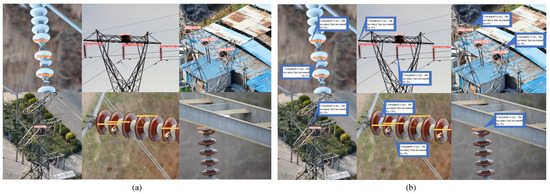
Figure 10.
(a) Detection performance of YOLOv5s. (b) Detection performance of EDF-YOLOv5.
Comparisons between the improved algorithm and the unimproved algorithm M0 lead to the following conclusions:
- (1)
- When using EN-SPPFCSPC alone to improve the algorithm, there is a slight improvement in the average detection accuracy of defect targets. The mAP@.5 increased by 0.9%. Although the detection speed decreased slightly, it still met the real-time detection standard.
- (2)
- When using DCNv3C3 alone to improve the algorithm, the algorithm can more accurately detect defects in power transmission lines. The mAP@.5 increased by 1.2%, and the F1 score also improved by 1.2%. This improvement effectively optimized the algorithm.
- (3)
- When using the Focal-CIoU loss function alone to improve the algorithm, there is a significant improvement in the average detection accuracy of defects in power transmission lines. The mAP@.5 increased by 1.5%, and there is also some improvement in the F1 score, while the detection speed remains unchanged. It is evident that the algorithm’s performance significantly improved.
- (4)
- When simultaneously using EN-SPPFCSPC and DCNv3C3 to improve the algorithm, the mAP@.5 increased by 1.2%, and there is some improvement in the F1 score. Although the detection speed is lower than the original algorithm, it still meets the real-time detection standard.
- (5)
- When simultaneously using Focal-CIoU and DCNv3C3 to improve the algorithm, the mAP@.5 increased by 1.0%, and the F1 score improved slightly, while the model’s detection speed decreased.
- (6)
- When simultaneously using the EN-SPPFCSPC and Focal-CIoU loss function to improve the algorithm, the mAP@.5 increased by 1.1%, and there is some improvement in the F1 score. Although the speed decreased by 31 frames per second, real-time detection was still guaranteed.
- (7)
- When simultaneously applying the three proposed improvement methods in this paper to the algorithm, the algorithm achieves optimal detection accuracy for defects in power transmission lines in this experiment. The mAP@.5 increased by 2.3%, and the F1 score improved by 0.8%. The detection speed decreased by 49 frames per second, but it did not affect the algorithm’s real-time performance. Furthermore, in conjunction with the detection results displayed in Figure 10, we can draw the following conclusions. It is evident that the EDF-YOLOv5 algorithm proposed in this paper performs better on the power transmission line defect dataset. Compared to the unimproved algorithm, it achieves a significant improvement in detection accuracy and can more accurately detect defect targets, demonstrating the effectiveness of the improvements proposed in this paper.
3.7. Comparison of Evaluation Metrics for Mainstream Object Detection Algorithms
To further validate the detection performance of the EDF-YOLOv5 algorithm on this dataset, we conducted comparative experiments with the current mainstream object detection algorithms, including Faster R-CNN, Mask R-CNN, SSD, YOLOX, and YOLOv8. The experimental results are presented in Table 6.
Table 6.
Performance comparison of mainstream detection algorithms.
From Table 6, the following conclusions can be drawn:
- (1)
- In terms of mAP@.5, EDF-YOLOv5 demonstrates an outstanding performance. It outperforms classical two-stage object detection algorithms, Faster R-CNN and Mask R-CNN, with accuracy improvements of 13.5% and 9.8%, respectively. Compared to other single-stage object detection algorithms, such as YOLOv5s, SSD, YOLOX, and YOLOv8, it achieves improvements of 2.3%, 12.0%, 7.5%, and 0.4%, respectively. This indicates that the algorithm exhibits superior detection effectiveness for power transmission line defects.
- (2)
- Analyzing the detection speed of the algorithms, it is observed that the two-stage object detection algorithm, Faster R-CNN, has the lowest detection speed. YOLOv8 achieves the fastest detection speed, reaching up to 181 frames per second, while EDF-YOLOv5’s detection speed of 117 frames per second ranks third among the compared algorithms. It is evident that EDF-YOLOv5 also possesses a certain advantage in terms of detection speed, meeting the real-time detection requirements.
- (3)
- The F1 score is another standard for assessing algorithm accuracy. Comparing the F1 scores of different object detection algorithms, it is noted that EDF-YOLOv5 achieves an F1 score of 90.1%. This is an improvement of 0.8%, 27.4%, 16.4%, and 0.7% compared to other object detection algorithms, including YOLOv5s, Faster R-CNN, SSD, and YOLOv8, respectively. It is evident that the EDF-YOLOv5 algorithm exhibits an outstanding performance in power transmission line defect detection, both in terms of detection speed and accuracy.
4. Conclusions
This paper introduces an improved YOLOv5s algorithm, EDF-YOLOv5, for the detection of power transmission line defects in aerial drone images. Through extensive experiments, it has been demonstrated that the proposed EN-SPPFCSPC module effectively utilizes comprehensive information from input features while controlling the parameter count, reducing the loss of fine-grained details, and improving the algorithm’s detection accuracy. The introduced DCNv3C3 module enhances the model’s generalization ability and synchronously improves detection accuracy. Additionally, the Focal-CIoU loss function enables the algorithm to achieve faster convergence and lower initial loss values. In summary, the enhanced algorithm exhibits superior performance in power transmission line defect detection tasks, achieving a mAP@.5 of 93.1% and an F1 score of 90.1%, with a detection speed of 117 frames per second, meeting the real-time detection requirements for power transmission line defect detection. Moving forward, we will continue to explore on the basis of this improved algorithm, make further efforts to enhance accuracy, and pursue algorithm lightweighting. We hope that the proposed improved algorithm can find broader applications in the field.
Author Contributions
Conceptualization, H.P. and Y.M.; methodology, H.P. and M.L.; formal analysis, H.P., M.L. and C.Y.; investigation, H.P. and C.Y.; data curation, H.P. and M.L.; writing—original draft preparation, M.L. and C.Y.; writing—review and editing, H.P. and Y.M.; visualization, H.P., M.L. and C.Y.; supervision, H.P. and Y.M. All authors have read and agreed to the published version of the manuscript.
Funding
This research was funded by the NSFC-Henan Joint Fund under Grant No. U1904119 and the Key Scientific Research Projects of Higher Education Institutions in Henan Province under Grant No. 23A520037.
Data Availability Statement
Data are contained within the article.
Conflicts of Interest
The authors declare no conflict of interest.
References
- Liu, C.; Wu, Y.; Liu, J.; Sun, Z.; Xu, H. Insulator faults detection in aerial images from high-voltage transmission lines based on deep learning model. Appl. Sci. 2021, 11, 4647. [Google Scholar] [CrossRef]
- Liu, Z.; Wu, G.; He, W.; Fan, F.; Ye, X. Key target and defect detection of high-voltage power transmission lines with deep learning. Int. J. Electr. Power Energy Syst. 2022, 142, 108277. [Google Scholar] [CrossRef]
- Liang, H.; Zuo, C.; Wei, W. Detection and evaluation method of transmission line defects based on deep learning. IEEE Access 2020, 8, 38448–38458. [Google Scholar] [CrossRef]
- Yang, H. Transmission Line Fault Detection Based on Multi-layer Perceptron. In Proceedings of the 2022 International Conference on Big Data, Information and Computer Network (BDICN), Sanya, China, 20–22 January 2022; pp. 778–781. [Google Scholar]
- Wanguo, W.; Zhenli, W.; Bin, L.; Yuechen, Y.; Xiaobin, S. Typical defect detection technology of transmission line based on deep learning. In Proceedings of the 2019 Chinese Automation Congress (CAC), Hangzhou, China, 22–24 November 2019; pp. 1185–1189. [Google Scholar]
- Zhao, W.; Xu, M.; Cheng, X.; Zhao, Z. An insulator in transmission lines recognition and fault detection model based on improved faster RCNN. IEEE Trans. Instrum. Meas. 2021, 70, 1–8. [Google Scholar] [CrossRef]
- Wang, J.; Deng, F.; Wei, B. Defect Detection Scheme for Key Equipment of Transmission Line for Complex Environment. Electronics 2022, 11, 2332. [Google Scholar] [CrossRef]
- Feng, Z.; Guo, L.; Huang, D.; Li, R. Electrical insulator defects detection method based on yolov5. In Proceedings of the 2021 IEEE 10th Data Driven Control and Learning Systems Conference (DDCLS), Suzhou, China, 14–16 May 2021; pp. 979–984. [Google Scholar]
- Li, Q.; Zhao, F.; Xu, Z.; Wang, J.; Liu, K.; Qin, L. Insulator and damage detection and location based on YOLOv5. In Proceedings of the 2022 International Conference on Power Energy Systems and Applications (ICoPESA), Virtual, 25–27 February 2022; pp. 17–24. [Google Scholar]
- Deng, F.; Xie, Z.; Mao, W.; Li, B.; Shan, Y.; Wei, B.; Zeng, H. Research on edge intelligent recognition method oriented to transmission line insulator fault detection. Int. J. Electr. Power Energy Syst. 2022, 139, 108054. [Google Scholar] [CrossRef]
- Wang, X.; Li, W.; Guo, W.; Cao, K. SPB-YOLO: An efficient real-time detector for unmanned aerial vehicle images. In Proceedings of the 2021 International Conference on Artificial Intelligence in Information and Communication (ICAIIC), Jeju Island, Republic of Korea, 13–16 April 2021; pp. 99–104. [Google Scholar]
- Souza, B.J.; Stefenon, S.F.; Singh, G.; Freire, R.Z. Hybrid-YOLO for classification of insulators defects in transmission lines based on UAV. Int. J. Electr. Power Energy Syst. 2023, 148, 108982. [Google Scholar] [CrossRef]
- Zaidi, S.S.A.; Ansari, M.S.; Aslam, A.; Kanwal, N.; Asghar, M.; Lee, B. A survey of modern deep learning based object detection models. Digit. Signal Process. 2022, 126, 103514. [Google Scholar] [CrossRef]
- Girshick, R. Fast r-cnn. In Proceedings of the IEEE International Conference on Computer Vision, Santiago, Chile, 7–13 December 2015; pp. 1440–1448. [Google Scholar]
- Ren, S.; He, K.; Girshick, R.; Sun, J. Faster r-cnn: Towards real-time object detection with region proposal networks. Adv. Neural Inf. Process. Syst. 2015, 28. [Google Scholar] [CrossRef]
- Cui, F.; Ning, M.; Shen, J.; Shu, X. Automatic recognition and tracking of highway layer-interface using Faster R-CNN. J. Appl. Geophys. 2022, 196, 104477. [Google Scholar] [CrossRef]
- Kim, J.H.; Kim, N.; Park, Y.W.; Won, C.S. Object detection and classification based on YOLO-V5 with improved maritime dataset. J. Mar. Sci. Eng. 2022, 10, 377. [Google Scholar] [CrossRef]
- Kim, J.; Sung, J.Y.; Park, S. Comparison of Faster-RCNN, YOLO, and SSD for real-time vehicle type recognition. In Proceedings of the 2020 IEEE International Conference on Consumer Electronics-Asia (ICCE-Asia), Seoul, Republic of Korea, 1–3 November 2020; pp. 1–4. [Google Scholar]
- Fang, W.; Wang, L.; Ren, P. Tinier-YOLO: A real-time object detection method for constrained environments. IEEE Access 2019, 8, 1935–1944. [Google Scholar] [CrossRef]
- Hu, C.; Min, S.; Liu, X.; Zhou, X.; Zhang, H. Research on an Improved Detection Algorithm Based on YOLOv5s for Power Line Self-Exploding Insulators. Electronics 2023, 12, 3675. [Google Scholar] [CrossRef]
- Han, G.; Yuan, Q.; Zhao, F.; Wang, R.; Zhao, L.; Li, S.; He, M.; Yang, S.; Qin, L. An Improved Algorithm for Insulator and Defect Detection Based on YOLOv4. Electronics 2023, 12, 933. [Google Scholar] [CrossRef]
- Bao, W.; Du, X.; Wang, N.; Yuan, M.; Yang, X. A Defect Detection Method Based on BC-YOLO for Transmission Line Components in UAV Remote Sensing Images. Remote Sens. 2022, 14, 5176. [Google Scholar] [CrossRef]
- Qiu, Z.; Zhu, X.; Liao, C.; Shi, D.; Qu, W. Detection of transmission line insulator defects based on an improved lightweight YOLOv4 model. Appl. Sci. 2022, 12, 1207. [Google Scholar] [CrossRef]
- Benjumea, A.; Teeti, I.; Cuzzolin, F.; Bradley, A. YOLO-Z: Improving small object detection in YOLOv5 for autonomous vehicles. arXiv 2021, arXiv:2112.11798. [Google Scholar]
- Zhou, F.; Zhao, H.; Nie, Z. Safety helmet detection based on YOLOv5. In Proceedings of the 2021 IEEE International Conference on Power Electronics, Computer Applications (ICPECA), Shenyang, China, 22–24 January 2021; pp. 6–11. [Google Scholar]
- Mahaur, B.; Mishra, K.K. Small-object detection based on YOLOv5 in autonomous driving systems. Pattern Recognit. Lett. 2023, 168, 115–122. [Google Scholar] [CrossRef]
- Wang, L.; Cao, Y.; Wang, S.; Song, X.; Zhang, S.; Zhang, J.; Niu, J. Investigation into recognition algorithm of helmet violation based on YOLOv5-CBAM-DCN. IEEE Access 2022, 10, 60622–60632. [Google Scholar] [CrossRef]
- Li, C.; Li, L.; Geng, Y.; Jiang, H.; Cheng, M.; Zhang, B.; Ke, Z.; Xu, X.; Chu, X. Yolov6 v3.0: A full-scale reloading. arXiv 2023, arXiv:2301.05586. [Google Scholar]
- Stergiou, A.; Poppe, R.; Kalliatakis, G. Refining activation downsampling with SoftPool. In Proceedings of the IEEE/CVF International Conference on Computer Vision, Montreal, BC, Canada, 11–17 October 2021; pp. 10357–10366. [Google Scholar]
- Wang, W.; Dai, J.; Chen, Z.; Huang, Z.; Li, Z.; Zhu, X.; Qiao, Y. Internimage: Exploring large-scale vision foundation models with deformable convolutions. In Proceedings of the IEEE/CVF Conference on Computer Vision and Pattern Recognition, Vancouver, BC, Canada, 18–22 June 2023; pp. 14408–14419. [Google Scholar]
- Zhang, Y.F.; Ren, W.; Zhang, Z.; Jia, Z.; Wang, L.; Tan, T. Focal and efficient IOU loss for accurate bounding box regression. Neurocomputing 2022, 506, 146–157. [Google Scholar] [CrossRef]

Disclaimer/Publisher’s Note: The statements, opinions and data contained in all publications are solely those of the individual author(s) and contributor(s) and not of MDPI and/or the editor(s). MDPI and/or the editor(s) disclaim responsibility for any injury to people or property resulting from any ideas, methods, instructions or products referred to in the content. |
© 2023 by the authors. Licensee MDPI, Basel, Switzerland. This article is an open access article distributed under the terms and conditions of the Creative Commons Attribution (CC BY) license (https://creativecommons.org/licenses/by/4.0/).