Abstract
The restoration of underwater images plays a vital role in underwater target detection and recognition, underwater robots, underwater rescue, sea organism monitoring, marine geological surveys, and real-time navigation. In this paper, we propose an end-to-end neural network model, UW-Net, that leverages discrete wavelet transform (DWT) and inverse discrete wavelet transform (IDWT) for effective feature extraction for underwater image restoration. First, a color correction method is applied that compensates for color loss in the red and blue channels. Then, a U-Net based network that applies DWT for down-sampling and IDWT for up-sampling is designed for underwater image restoration. Additionally, a chromatic adaptation transform layer is added to the net to enhance the contrast and color in the restored image. The model is rigorously trained and evaluated using well-known datasets, demonstrating an enhanced performance compared with existing methods across various metrics in experimental evaluations.
1. Introduction
Underwater imaging is important for many underwater activities, like visual surveys, which need clear and accurate images. However, underwater images are usually less clear, have a low contrast, contain noise, and look hazy due to the absorption and scattering of the direction of light. In normal seawater images, it is common for objects that are more than 10 m away to be almost impossible to see clearly, and their colors also become less vibrant as they move deeper into the water. Underwater image enhancement (UIE), i.e., color restoration, enhancing the contrast, and details, is an essential task in marine engineering and observation applications [1].
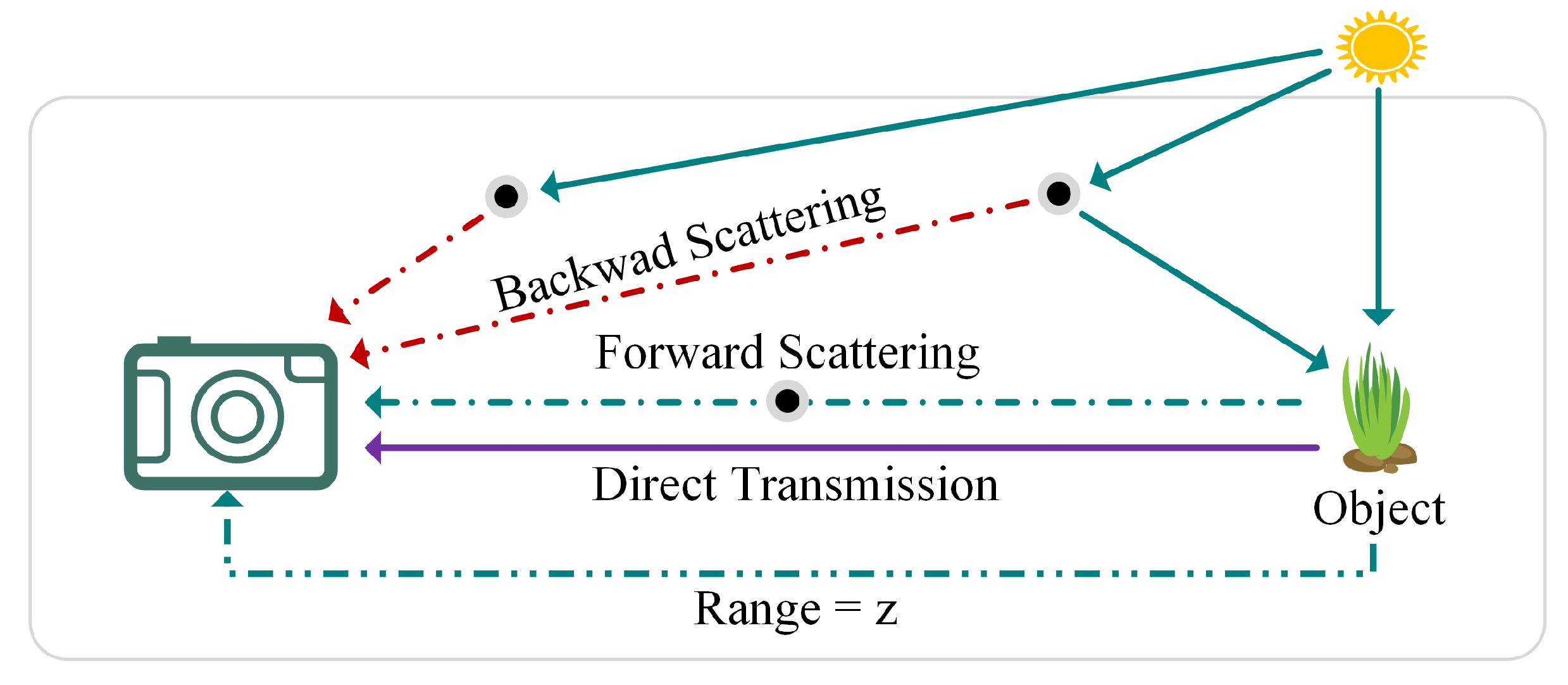
The formation of underwater images is illustrated in Figure 1, where three different types of light are observed as reaching the imaging device: (1) direct transmission, which travels directly to the camera after striking the object; (2) forward-scattered light, which deviates from its original path upon interacting with the object; and (3) back-scattered light, which reaches the camera after encountering particles in the water. The attenuation of light is influenced by both the distance between the device and the object, as well as the light’s wavelength, and is further affected by seasonal, geographic, and climatic variations [2]. These factors collectively impose significant challenges on the quality of captured images, making image restoration a challenging task. The atmospheric scattering model is a traditional way to explain how hazy images are created [3,4].
where , is the hazy image, is the scene radiance, is the background light, and is the transmission map, for each of the RGB color channels. The transmission map can be written as . Here, is the attenuation coefficient for each color channel and is the distance between the observer and the object.
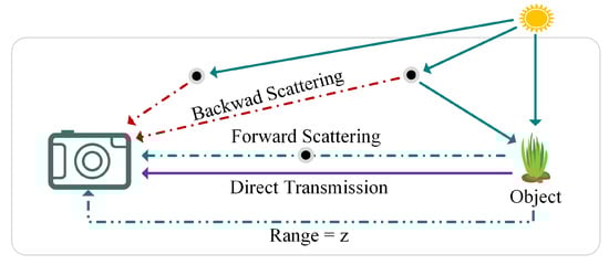
Figure 1.
Illustration of underwater image formation, showing the camera receiving three types of light: direct reflected light, forward-scattered light, and back-scattered light.
A wide range of techniques have been developed to tackle the challenges in underwater image enhancement, which can be broadly categorized into traditional and deep learning approaches. Traditional methods, such as those in [5,6,7,8,9,10,11,12,13,14,15], focus on modeling and correcting the specific distortions encountered in underwater environments. They often rely on physical models to correct specific distortions by estimating light scattering and absorption. However, these methods often struggle with different water types due to their reliance on static models. The Sea-thru model [16] presents a revised model accounting for varying attenuation and scattering behaviors:
where is the observed intensity, is the inherent radiance, is the ambient light, and are the attenuation coefficients, and z is the distance. The vectors and represent dependencies, with as the reflectance, E as the irradiance, as the sensor response, b as the backscatter, and as the scattering and attenuation coefficients.
To further refine underwater image formation, recent complex imaging models like [17] offer improvements by capturing differential absorption and scattering effects:
with being the observed intensity, as the source radiance, and as the ambient light. These models focus on the dominant distance effect on image degradation without needing detailed depth or manual optical parameters.
On the other hand, deep learning techniques, such as those in [18,19,20,21,22,23,24], leverage the power of neural networks to learn complex mappings from degraded underwater images in order to their enhanced counterparts. These methods have shown promising results in handling diverse underwater image distortions, offering adaptability and generalization capabilities across different datasets [1,21,25,26]. Despite their effectiveness, they require extensive, annotated training data and computational resources, posing challenges for practical deployment, especially in dynamically changing underwater environments.
In this paper, we introduce UW-Net, a comprehensive end-to-end neural network model specifically designed for underwater image restoration. This model uniquely combines color correction techniques with discrete wavelet transform (DWT) and inverse discrete wavelet transform (IDWT), as well as incorporating a chromatic adaptation layer for enhanced image quality. The key contributions of our research are summarized as follows:
- Development of UW-Net, a neural network model leveraging DWT and IDWT for enhanced feature extraction, tailored specifically for underwater image restoration tasks.
- Implementation of a color correction method that effectively addresses color loss in the red and blue channels, utilizing the Gray World Hypothesis to significantly enhance the visual quality of the restored images.
- Integration of a chromatic adaptation layer within UW-Net, which significantly improves the contrast and color fidelity of the output images, resulting in a noticeable enhancement in the overall image quality.
2. Related Work
In the literature, there have been numerous efforts to enhance visibility and restore the quality of degraded underwater images. These techniques are generally categorized into traditional and learning-based methods. Traditional methods improve image clarity by calculating atmospheric light and creating a transmission map. They often employ various strategies, such as guided filtering, statistical models, and matting algorithms, to refine the initial transmission map. Typically, key parameters in the image formation model are inferred using various man-made principles or ‘priors’; these are then used to reverse the model, producing a clear image. Notable priors include the dark channel prior [5], which leverages the observation that most local patches in haze-free images have low-intensity pixels in at least one color channel, allowing for the direct estimation of haze thickness and the recovery of high-quality haze-free images, and the underwater dark channel prior [6], which focuses on green and blue channels for transmission estimation in underwater images. Additionally, the Histogram Distribution Prior [7] proposes an algorithm based on the minimum information loss principle to enhance contrast and brightness. The two-step approach [8] enhances underwater image quality in two phases, addressing color distortion and low contrast separately. The blurriness prior [9] introduces a depth estimation method for underwater scenes based on image blurriness and light absorption. Non-local dehazing [10] detects haze lines automatically and uses them for dehazing. The generalized dark channel prior (GDCP) [27] estimates ambient light using depth-dependent color changes and calculates scene transmission based on the observed intensity differences. The region line prior [28] transforms the dehazing process into a 2D joint optimization function, leveraging information across the entire image for reliable restoration. While effective in some scenarios, the reliance of these physics-based methods on man-made priors often limits their effectiveness in handling the diverse optical properties of water.
Beyond prior-based methods, novel approaches have emerged. UTV [11] restores images using the underwater dark channel prior (UDCP) within a variational framework, enhancing dehazing, contrast, and edge preservation, while suppressing noise. Moreover, TEBCF [12] merges different scales of an image to enhance texture. CBM [13] focuses on restoring scene object details for improved visual results. WWPF [15] combines color correction and contrast adjustments to address common issues in underwater image quality. UNTV [29], which combine the total variation and blur kernel sparsity into a unified framework uses efficient algorithms for transmission map refinement, background light estimation, and accelerated convergence. MMLE [30] proposes a locally adaptive color correction method built on the minimum color loss principle and the maximum attenuation map-guided fusion strategy. These methods represent a significant evolution in tackling the specific challenges of underwater imaging. Recently, PCDE [14] introduced a piece-wise color correction technique utilizing dual gain factors for adaptive color balancing and a dual prior optimized strategy for contrast enhancement that separately optimizes the base and detail layers of the image to improve the overall quality.
Deep learning, with its powerful convolutional neural networks (CNNs), generative adversarial networks (GANs), and other advanced neural networks, has revolutionized underwater image enhancement. These technologies have led to a surge in specialized and effective methods tailored for the unique challenges presented by underwater environments. UcycleGAN, developed by [18], employs a semi-supervised approach for color adjustment and haze removal in underwater images. Fabbri et al. furthered this field with UGAN [19], a GAN-based method that significantly enhances the visual quality of underwater scenes, proving particularly beneficial for autonomous underwater vehicles in generating clear imagery from obscured underwater environments. In addition, the UWCNN model by [20] stands out as a lightweight yet effective solution for improving both underwater images and videos. This model capitalizes on specialized training data to directly enhance image quality. Complementing this, Water-Net [21], also by Li et al., not only offers a comprehensive dataset of real-world underwater images for benchmarking purposes, but also introduces an innovative model trained on this dataset to further advance image enhancement techniques. MDGAN, conceptualized by [22], utilizes the prowess of GANs to refine image details, employing an intricate block system and specialized training regimen. Similarly, FUnIE-GAN by [23] was designed for rapid underwater image enhancement, focusing on augmenting overall visual quality, color richness, and texture clarity. The Ucolor method by [24] takes a novel approach, harnessing various color spaces and an attention mechanism to specifically target and enhance the most quality-degraded areas of underwater images. Moreover, the PUIE model by [31] employs a sophisticated autoencoder framework, demonstrating the breadth and adaptability of deep learning techniques in understanding and enhancing the quality of underwater imagery. More recently, new frameworks like SyreaNet [32] and SCEIR [33] have been proposed for underwater image enhancement and restoration. SyreaNet, a GAN-based technique, fuses synthetic and real data with advanced domain adaptation to enhance underwater image restoration. SCEIR introduces a two-part underwater image restoration model: one module for global color and contrast correction, another for local detail enhancement, based on the atmospheric scattering model principles. These diverse methodologies underscore the significant impact and potential of learning-based methods, offering significant improvements in both the technical approach and the quality of image restoration.
Quality Evaluation in Image Super-Resolution
Recent advancements in image super-resolution (SR), driven by deep learning and transformer-based models, have underscored the importance of accurately evaluating the quality of super-resolved images, surpassing the capabilities of traditional standards [34,35]. Conventional metrics such as PSNR, SSIM, NIQE, and their variants provide quantitative assessments, but may not fully capture the perceptual nuances that human observers can appreciate [36]. To overcome these limitations, specialized SR quality metrics have emerged. The DeepSRQ network, for example, scrutinizes the structural and textural aspects of quality separately, which enhances the feature representation of distorted images for a more discriminating analysis [36]. Additionally, the SRIF index introduces a two-dimensional evaluation that contrasts deterministic fidelity (DF) and statistical fidelity (SF), offering a holistic assessment of SR image quality [37]. This index synthesizes considerations of sharpness and texture into a comprehensive measure that reflects both the accuracy of detail and the naturalness of appearance. In addition, advancements have also addressed challenges in quality assessment related to image degradation and misalignment. DR-IQA, for instance, utilizes degraded images as references to establish a degradation-tolerant feature space, aligning features with pristine-quality images [38]. Similarly, LPIPS has been fine-tuned for greater tolerance to shifts, incorporating anti-aliasing filters and network structure alterations to align more closely with human visual perception, even in the presence of imperceptible misalignments [39]. These advancements in SR quality metrics represent a significant shift towards more human-centric evaluation methods, keeping pace with the rapid advancements in image enhancement and restoration algorithms.
3. Proposed Method
The proposed method for underwater image restoration involves compensating the red and blue channels using the green channel, extracting features with DWT and IDWT within UW-Net, and enhancing image brightness adaptively with a chromatic adaptation layer for better color restoration.
3.1. Color Correction
Given a degraded image , the color corrected image through the additive factors can be formulated as follows:
where denotes the constants for each channel, and signifies the scaling factor, which is determined based on the channel’s mean values. This determination is grounded in the principles of the Gray World Hypothesis [40], which assumes that, prior to distortion, all channels exhibit similar mean intensities. Thus, can be computed as follows:
where , , and denote the mean values of their respective channels of .
3.2. Wavelet Transform
Wavelet analysis has strengthened its role in image processing due to its ability to adeptly partition an image’s information into two integral categories: approximations, encapsulating broader trends, and details. This segregation is achieved using high-pass and low-pass filters, ending in the extraction of both the high-frequency (detail) and low-frequency (approximation) components of the image. When it comes to 2D DWT, the input signal is split into four distinguished filter bands: low-low (LL), low-high (LH), high-low (HL), and high-high (HH). For instance, the scaling function of a 2D wavelet, denoted by , is expressed as follows:
Given this, the other three 2D wavelets can be represented as follows:
where and denote the 1D scaling and wavelet functions along the x direction, respectively, and and are their counterparts along the y-direction, respectively.
In image processing, the 2D DWT operation is executed by sequentially applying 1D wavelet transforms—specifically, and —first across each row and then across each column of the color-corrected image . This method integrates both filtering and data reduction, which is commonly referred to as downsampling. Let the discrete wavelet transform function be denoted by W; this two-step operation can be generalized as follows:
where the symbol ∘ denotes the function composition, and and represent the 1D wavelet transforms applied row-wise and column-wise, respectively. The resulting 2D wavelet-transformed image, denoted as , yields four distinct, downscaled sub-band images: contains the low-frequency components, depicting broader image trends, whereas , , and capture the high-frequency details corresponding to the horizontal, vertical, and diagonal edges of the original color-corrected image, respectively. Conversely, IDWT employs these filters to reconstruct the wavelet-transformed image back to its original state. This approach utilizes both filtering and data upscaling, commonly known as upsampling. In the subsequent section, we elucidate how DWT and IDWT are employed in our model to extract enriched features in conjunction with convolution layers while managing the downsampling and upsampling of the image.
3.3. UW-Net Model
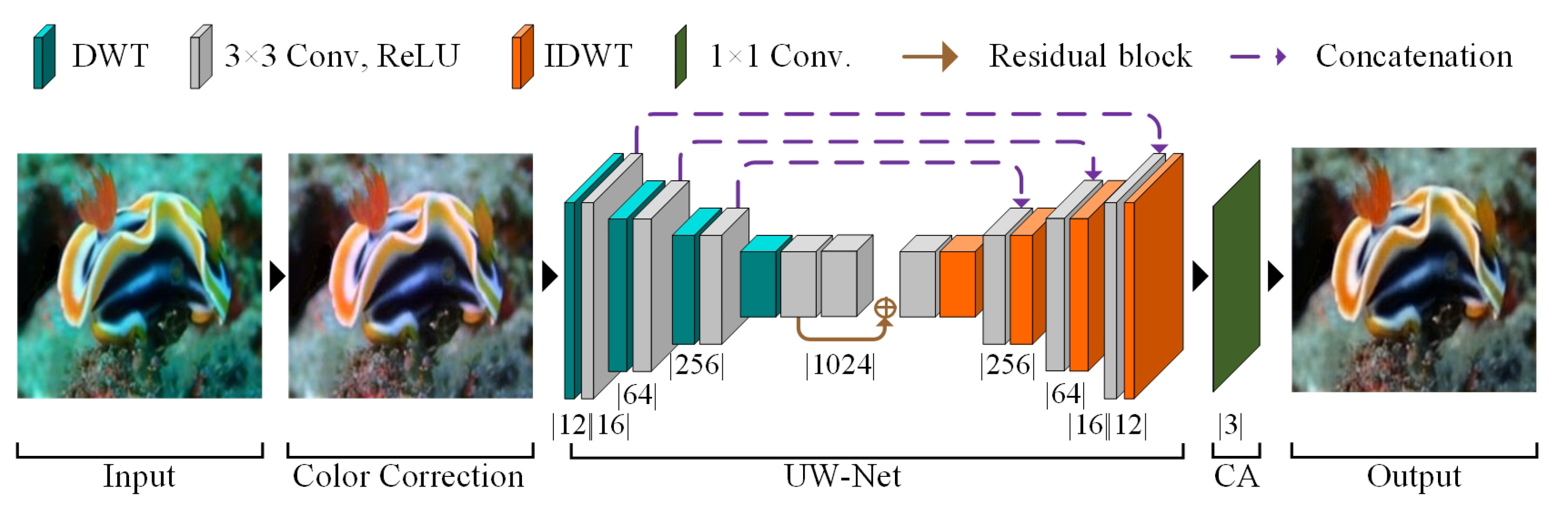
In our proposed underwater image dehazing network (UW-Net), we enhanced the U-Net architecture [41] by integrating both the discrete wavelet transform (DWT) and the inverse discrete wavelet transform (IDWT), as illustrated in Figure 2. The color-corrected image is provided to the UW-Net as the input. First, the DWT is applied to the color-corrected image , as detailed in Equations (4) and (5), thereby converting the image into a 12-channel representation. Each channel corresponds to one of the four sub-band images, as elaborated in Equation (6). These channels are then fed into a first convolutional layer , which expands the dimensions to 16 channels. The combined operation of applying DWT followed by the convolutional layers can be mathematically expressed as follows:
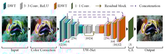
Figure 2.
Representation of the wavelet-based UW-Net integrating color correction and chromatic adaptation for effective single-image dehazing. Beneath each convolution layer, the number of output channels is denoted.
Here, represents the output with d channels, denotes the DWT funtional, represents the convolution kernel of size , and ⊛ indicates the convolution operation. Sequentially, we continue to downsample the input by half, resulting in dimensions of [128, 64, 32, 16], given the original input size of , while simultaneously multiplying the number of channels by 4, resulting in output channels [64, 256, 1024] for layers (). This approach resembles common practices of reducing data dimensions through adjusting convolution strides, but aims to preserve fine edge details that are often lost due to data discarding. Additionally, we consistently use padding and a stride of 1 throughout the network.
In addition to the downsampling of data, the U-Net architecture’s core includes a residual block, inspired by ResNet [42], designed to learn residual functions with respect to the input layers. This facilitates the training of deeper networks. The operations involving the residual and convolutional layers are represented as follows:
where is the output with d channels obtained after the residual operation, ⊕ symbolizes element-wise addition, and represents the convolution kernels of size . Here, denotes the output from the last downsampled convolutional layer , and refers to the output of the subsequent convolutional layer .
After residual processing, the output is upsampled and reconstructed using IDWT to refine the previously outlined edge features by applying layers (). At layer , the combined operation of applying the convolutional and IDWT is mathematically expressed as follows:
where is the output with d channels, denotes the IDWT functional, and is the convolution operation with a size of . This upsampling continues through layers (). At each layer, the output channel’s dimensions are doubled and the channel numbers are reduced times. Thus, the original input channel dimensions are retrieved, while reducing the number of channels by a factor of four, returning to 16 channels. Following the final convolution layer , the resultant image is transformed back to 12-channel dimensions. Finally, the operation is applied as follows:
Here, represents the output image obtained from the last IDWT and the convolution filter of size . Note that the output of the layer has channels.
The UW-Net model, tailored for underwater image dehazing, boasts a significant depth with approximately 30.2 million trainable parameters. In terms of computational demands, the model requires an input size of 0.75 MB per image, and the total memory footprint for processing each image, including the forward and backward pass, is around 157.97 MB. This encompasses a forward/backward pass size of 42.00 MB and a parameter memory requirement of 115.22 MB. The next segment of UW-Net, which involves a chromatic adaptation layer (CA), is detailed in the subsequent section.
3.4. Image Restoration
Color restoration is pivotal for enhancing the visual quality of dehazed images produced by UW-Net, in addition to edge delineation. The images, particularly those emerging from the final layer of UW-Net, often exhibit a diminished luminance. To counteract this, a chromatic adaptation (CA) layer is integrated to adjust the color balance and enhance brightness. Drawing on the statistical-based simplified model presented in [43], we employ a standardized matrix to uniformly and adaptively improve the contrast of the final output image . The mathematical representation of this operation is as follows:
where the diagonal matrix, with diagonal elements , , and , being greater than zero, is utilized to scale the respective color channels. The color transformation process, as delineated in Equation (13), exhibits a resemblance to the functionality of a residual block. In this context, the transformation is effected through a convolutional kernel, catering to both the input and output of the 3-channel images. The initialization range of the convolutional kernels, set between 0 and 1, not only accelerates the learning process by mitigating the diagonal elements, but also enhances the precision of the model. This enhancement is attributable to the intrinsic accuracy-improving characteristics of the residual block.
4. Results and Discussions
4.1. Experimental Setup
In our experimental setup, the proposed UW-NET model is rigorously evaluated using the EUVP (Enhancing Underwater Visual Perception) dataset [23]. The EUVP dataset, specifically designed for underwater image enhancement, comprises a comprehensive collection of both paired and unpaired images, showcasing a wide range of perceptual qualities. These images have been captured using seven different cameras under diverse visibility conditions, including during oceanic explorations and human–robot collaborative experiments. For training UW-NET, we utilized a subset comprising 9250 paired images from the Underwater Dark and Underwater ImageNet collections. Additionally, for validation purposes, the Underwater Scenes subset, containing 2185 images, was employed. The network underwent 110 epochs of training on this dataset. The training phase was facilitated by the Adam optimizer [44] with an initial learning rate of . Finally, for comprehensive testing and performance evaluation, 515 images from the test_samples folder, also a part of the EUVP dataset, were used, applying the same training parameters.
Furthermore, we included the Large Scale Underwater Image (LSUI) dataset [1], which offers an even more abundant and varied collection of underwater scenes compared with existing datasets. The LSUI dataset is comprised of 4279 real-world underwater image groups. Each group in the dataset provides a raw underwater image along with a clear reference image, enabling a direct comparison of the enhancement results. For the training of UW-NET using the LSUI dataset, we randomly selected 3879 picture pairs as the training set and reserved the remaining 400 for the test set, undergoing 200 epochs of training. Each image was resized to 240 × 320 pixels for uniformity. The same Adam optimizer with an initial learning rate of was employed throughout the training phase. The LSUI dataset’s provision of high-quality reference images and additional image processing maps presented a unique opportunity to evaluate UW-NET’s performance in enhancing underwater imagery with greater accuracy and context awareness.
Moving to the specifics of the model training, all of the model parameters were initialized randomly, and RMSE was employed as the primary loss metric. The use of RMSE aligned with our objective to minimize the errors between the estimated output images and the ground truth images, ensuring a high fidelity in the restored underwater imagery.
4.2. Evaluation Metrics
In assessing the quality of restored images, we adopted widely recognized metrics such as RMSE, PSNR, and SSIM [45], and the no-reference metric NIQE, introduced by Mittal et al. [46]. RMSE was calculated as follows:
where M and N represent the dimensions of the images, is the color-corrected input image, and is the output image. A lower value of RMSE indicates better results. In addition to RMSE, the peak signal-to-noise ratio (PSNR) was used as an evaluation metric during the validation phase. PSNR is a standard measure for assessing the quality of reconstructed images in comparison with the original ones. PSNR was calculated using the formula:
where is the maximum possible pixel value of the image, and MSE represents the mean squared error, calculated as the squared difference between and , averaged over all of the pixels. A higher value of PSNR represented better quality.
For assessing the perceptual quality of the output images, the Structural Similarity Index (SSIM) was used:
where and are the average pixel values, and are the variances, and is the covariance of the input and output images, respectively. SSIM values ranged from −1 to 1, with 1 indicating perfect similarity.
Lastly, the Naturalness Image Quality Evaluator (NIQE) was applied as a no-reference image quality assessment:
where is a function that quantifies the naturalness of the restored output image by measuring its statistical deviations from established natural image statistics. Lower NIQE values denote a higher resemblance to the quality of natural scenes.
4.3. Comparative Analysis
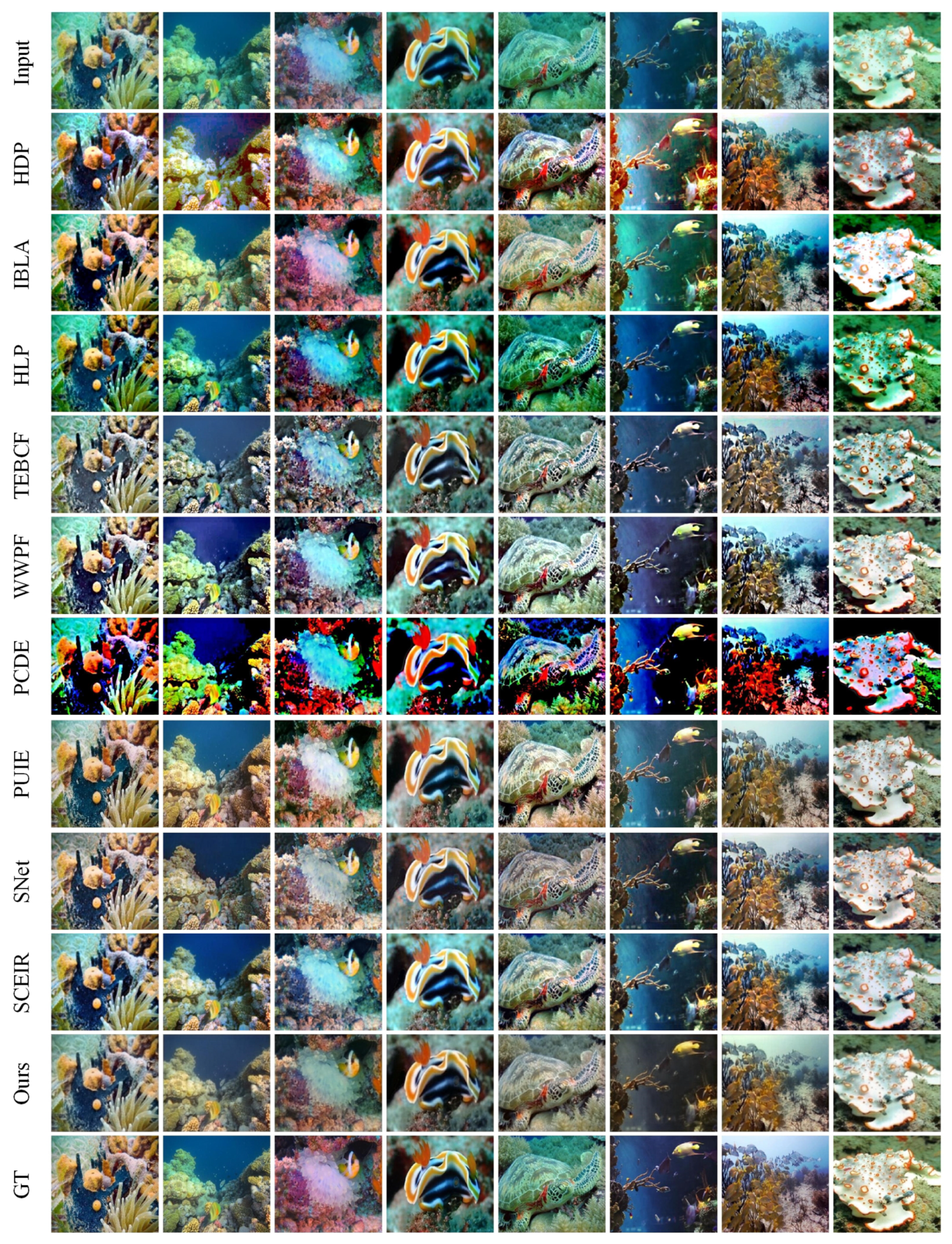
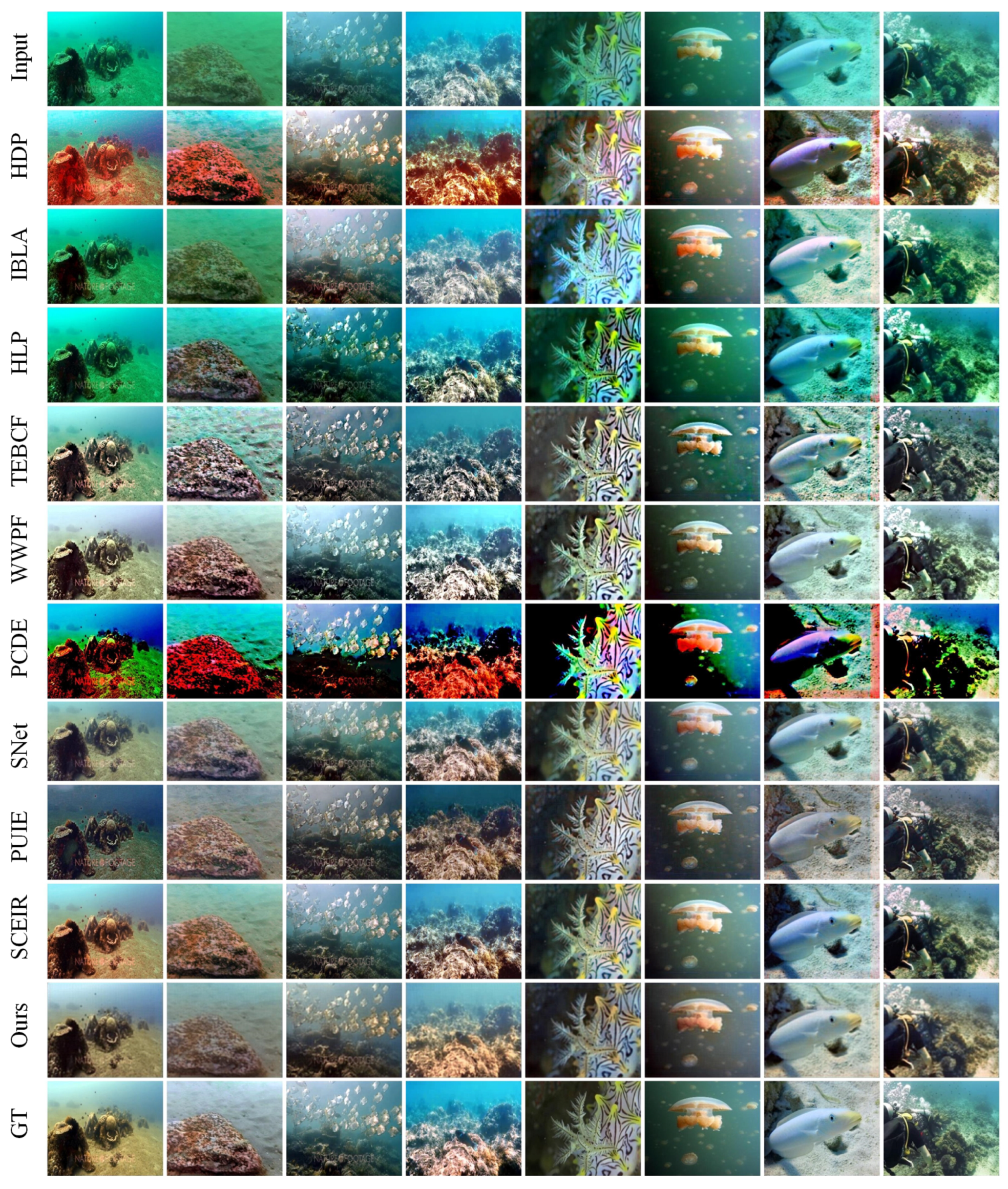
In this study, we assessed the performance of several underwater image enhancement techniques, including our proposed method, through both qualitative and quantitative evaluations. We employed real-world hazy images from the EUVP test_samples for a comparative analysis. Initially, eight random test images were restored using various methods: HDP [7], IBLA [9], HLP [10], TEBCF [12], WWPF [15], PCDE [14], PUIE [31], SNet [32], SCEIR [33], and our proposed method. The results, displayed in Figure 3, reveal that images enhanced using our method generally exhibited a better quality. A detailed examination shows that HDP [7] and PCDE [14] often introduced significant color distortion and texture degradation. On the other hand, methods like HLP [10] and TEBCF [12] struggled to completely eliminate haze effects. Although WWPF [15] performed better compared with other non-learning methods, it still exhibited color loss relative to the ground truth (GT). In contrast, learning-based methods such as PUIE [31], SNet [32], SCEIR [33], and our proposed technique consistently produced higher quality restorations. These methods effectively preserved texture, maintained color balance, and aligned more closely with GT. Overall, the comparative analysis presented in Figure 3 highlights the good performance of learning-based approaches over traditional or non-learning methods, including the proposed method, which consistently demonstrates an enhanced image quality across a range of challenging underwater conditions.
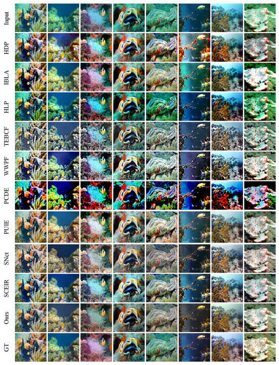
Figure 3.
Comparative analysis of dehazing methods on the EUVP dataset test images. This figure illustrates a progression from top to bottom: the original input image, followed by outcomes from non-learning-based methods HDP [7], IBLA [9], HLP [10], TEBCF [12], WWPF [15], and PCDE [14], as well as learning-based approaches such as PUIE [31], SNet [32], SCEIR [33], our method, and the ground truth. The figure presents the nuanced performance of various dehazing techniques, with the learning-based methods showing competitive results, including the proposed method.
The quantitative analysis of the EUVP dataset and samples, as shown in Figure 3, is detailed in Table 1, where the performance of both non-learning and learning-based image enhancement methods is compared using RMSE, SSIM, PSNR, and NIQE metrics. Within the non-learning methods, WWPF showed the lowest RMSE of 0.08 and highest PSNR of 21.52 dB. IBLA, on the other hand, achieved the highest SSIM of 0.84. PCDE recorded the lowest NIQE score of 3.24, suggesting its enhanced naturalness in image quality. In contrast, the learning-based methods demonstrated even more robust performances. PUIE achieved both the lowest RMSE of 0.10 and the highest SSIM of 0.96. The proposed method outperformed in PSNR with a high of 24.60 dB, underlining its superiority in the peak signal-to-noise ratio. Furthermore, it maintained a balanced performance in NIQE scores, ranging from 4.02 to 6.05 across various tests. Overall, while the learning-based methods generally excelled over non-learning ones, each technique exhibited unique strengths.

Table 1.
Comparative evaluation of image enhancement methods on the EUVP dataset, using RMSE, SSIM, PSNR, and NIQE metrics. Lower RMSE/NIQE and higher SSIM/PSNR indicate better image quality.
We next evaluated the effectiveness of our proposed method against a range of well-known techniques using challenging images from the LSUI dataset. For this comparative analysis, eight randomly selected test images were enhanced using several methods, such as HDP [7], IBLA [9], HLP [10], TEBCF [12], WWPF [15], PCDE [14], PUIE [31], SNet [32], and SCEIR [33], alongside our proposed technique. The results, depicted in Figure 4, indicate that our method typically yielded better image enhancement. A detailed analysis showed that HDP [7] and PCDE [14] tended to cause notable color distortion and texture degradation. In contrast, HLP [10] and IBLA [12] struggled with residual haze. WWPF [15], while improved over other non-learning methods, still faced color fidelity issues compared with the ground truth (GT). Among learning-based methods, PUIE [31] sometimes resulted in over-darkening of the images, but SNet [32] and SCEIR [33] delivered visually appealing restorations. Our proposed method also achieved high-quality restorations, effectively preserving the texture and color balance, and closely aligning with GT. Overall, learning-based approaches, including ours, exhibited a better performance compared with traditional methods.
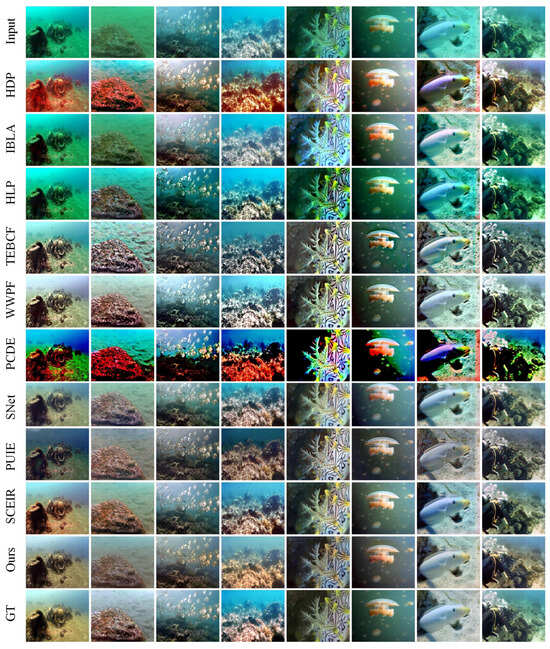
Figure 4.
Comparative analysis of dehazing methods on LSUI dataset test images. This figure illustrates a progression from the top to bottom: the original input image, followed by outcomes from non-learning-based methods HDP [7], IBLA [9], HLP [10], TEBCF [12], WWPF [15], PCDE [14], and learning-based approaches such as PUIE [31], SNet [32], SCEIR [33], our method, and the ground truth. The figure presents the nuanced performance of various dehazing techniques, with learning-based methods showing competitive results, including the proposed method.
The quantitative analysis for the samples from EUVP dataset LSUI dataset, as shown in Figure 3 and Figure 4, is detailed in Table 1 and Table 2, respectively, where the performance of both non-learning and learning-based image enhancement methods is compared using RMSE, SSIM, PSNR, and NIQE metrics. Among the non-learning methods, WWPF notably achieved the lowest RMSE of 0.05 and the highest PSNR at 25.40 dB. IBLA excelled with the highest SSIM score of 0.87, while HDP recorded the lowest NIQE score of 3.21. Shifting focus to the learning-based methods, SNet peformed better with the lowest RMSE of 0.02, the highest SSIM of 0.97, and PSNR of 33.06 dB. PUIE, meanwhile, had the lowest NIQE score of 2.72, indicative of its ability to produce naturally appearing images. Our proposed method demonstrated a balanced performance across the board, achieving an RMSE as low as 0.05, an SSIM up to 0.75, a PSNR of 26.30 dB, and maintaining NIQE scores within the range of 3.54 to 5.04 across different images. In summary, while learning-based methods generally surpassed their non-learning counterparts in terms of metric performance, each method exhibited its unique strengths.
Table 2.
Comparative evaluation of image enhancement methods on the LSUI dataset, using RMSE, SSIM, PSNR, and NIQE metrics. Lower RMSE/NIQE and higher SSIM/PSNR indicate better image quality.
In addition, a comprehensive quantitative evaluation was conducted using all of the test datasets. The EUVP test dataset comprised 515 images, while the LSUI dataset included 400 test images. Various methods were employed for image restoration, including HDP [7], IBLA [9], TEBCF [12], WWPF [15], PCDE [14], PUIE [31], SNet [32], SCEIR [33], and our proposed method. With the available ground truth data, RMSE, PSNR, SSIM, and NIQE metrics were computed for each restored image, and the average values for each method are summarized in Table 3. For the EUVP dataset among non-learning methods, TEBCF achieved the lowest RMSE of 0.14 and shared the highest SSIM of 0.63 with WWPF. IBLA recorded the highest PSNR of 17.32 and the lowest NIQE of 4.997. In the learning-based category, both PUIE and our proposed method achieved the lowest RMSE of 0.11, while SCEIR exhibited the highest SSIM of 0.68 and the lowest NIQE of 4.93. Our method demonstrated the highest PSNR of 19.90.
Table 3.
Quantitative comparison of non-learning and learning-based methods using RMSE, PSNR, SSIM, and NIQE metrics on the EUVP and LSUI datasets. Lower RMSE and NIQE and higher SSIM and PSNR indicate a better image quality.
For the LSUI dataset, TEBCF again showed the lowest RMSE of 0.13 among the non-learning methods, while WWPF had the highest SSIM of 0.71 and the highest PSNR of 18.10, IBLA achieved the lowest NIQE of 4.16. In the learning-based methods, SCEIR outperformed the others with the lowest RMSE of 0.10, the highest SSIM of 0.75, and the highest PSNR of 20.70, as well as a competitive NIQE of 4.22. The proposed method demonstrated a reasonable performance across all metrics, particularly in RMSE and PSNR, which were just slightly lower than those of SCEIR. Overall, while learning-based methods generally exhibited a superior performance, with SCEIR performing better in the LSUI dataset, non-learning methods like IBLA and TEBCF showed good results in specific metrics. The proposed method demonstrates a balanced performance, achieving competitive RMSE and the highest PSNR in the EUVP dataset, thus ensuring its viability as an effective image enhancement technique.
4.4. Ablation Study
In our ablation study, we meticulously analyzed the restored images both qualitatively and quantitatively using the EUVP and LSUI datasets. First, the average results for the complete test samples was computed from the EUVP and LSUI datasets with and without the color correction (CC) and chromatic layer (CL), as detailed in Table 4. It is evident that for both datasets, when the model was trained without CC, RMSE increased, while the PSNR and NIQE decreased, and the SSIM exhibited a mixed behavior. Conversely, the impact of CL on our proposed model’s performance was more pronounced. There was a significant difference in all of the metrics, highlighting CL’s effectiveness in enhancing the structure, color balance, and texture of the restored images.
Table 4.
Ablation study for average score comparison using different metrics with (w/) and without (w/o) color correction (CC) and chromatic layer (CL) on EUVP and LSUI datasets. ✓ indicates ‘yes’ and (×) represents ‘no’.
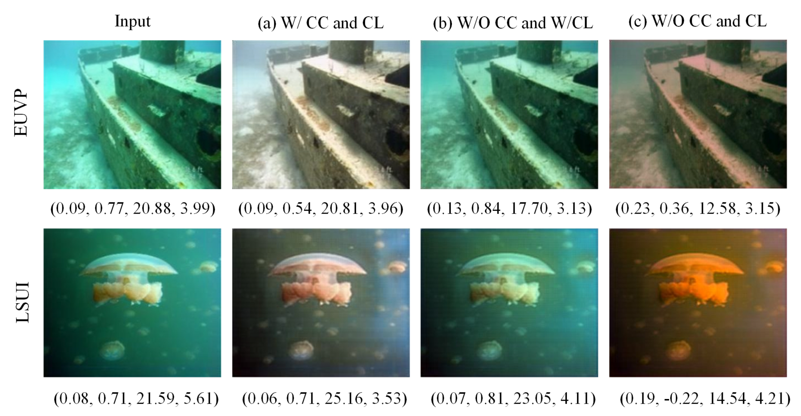
Furthermore, we selected two random images from each dataset to analyze the effect of CC and CL qualitatively and quantitatively, as depicted in Figure 5. Figure 5a demonstrates that the image restored with both the color correction (CC) and chromatic layer (CL) appears clear, without haze, and is visually appealing. Conversely, Figure 5b shows that employing CL without CC results in a restored image that retains some haze. Moreover, omitting both CC and CL, as observed in Figure 5c, produces an image with a pronounced reddish tint. The metrics, RMSE, SSIM, PSNR, and NIQE, listed below each image quantify the differences in performance with and without the use of CC and CL in our proposed model.
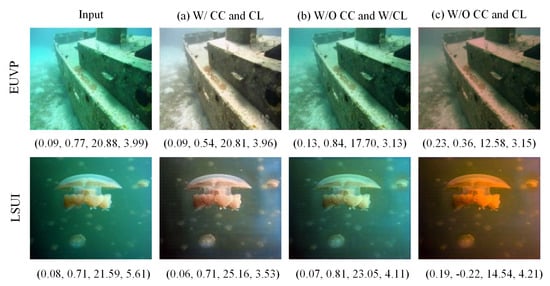
Figure 5.
Ablation study effects on underwater image restoration: comparative visualization using different metrics with (w/) and without (w/o) color correction (CC) and chromatic layer (CL) on the EUVP and LSUI datasets. Below each image, the corresponding metrics—RMSE, SSIM, PSNR, and NIQE—are provided to quantify the restoration quality.
5. Conclusions
In this work, we introduced an end-to-end neural network model utilizing discrete wavelet transform (DWT) and inverse discrete wavelet transform (IDWT) for the advanced feature extraction required for underwater image restoration. Our model incorporates a color correction strategy that effectively mitigates color losses, specifically in the red and blue channels. Further, we integrate a chromatic adaptation transform layer into UW-Net, which significantly increases contrast and color fidelity, yielding a noticeable enhancement in overall image quality. The ablation study further underscores the enhancement brought about by the synergistic effects of color correction and chromatic adaptation. Rigorous training and validation on the EUVP and LSUI datasets demonstrate that, while our model shows better performance in metrics like RMSE and PSNR, its results in perceptual quality metrics are competitive, but do not consistently surpass existing methods. Future work will aim to refine the model for optimized real-time performance and efficacy in varied underwater conditions, while developing a combined loss approach that balances traditional and perceptual quality metrics.
Author Contributions
Conceptualization, H.S.A.A. and M.T.M.; methodology, M.T.M.; software, H.S.A.A.; validation, H.S.A.A. and M.T.M.; formal analysis, H.S.A.A.; investigation, H.S.A.A.; resources, M.T.M.; data curation, H.S.A.A.; writing—original draft preparation, H.S.A.A.; writing—review and editing, M.T.M.; visualization, H.S.A.A.; supervision, M.T.M.; project administration, M.T.M.; funding acquisition, M.T.M. All authors have read and agreed to the published version of the manuscript.
Funding
This work was supported by the Education and Research Promotion Program of KoreaTech (2023) and by the Basic research program through the National Research Foundation (NRF) Korea grant funded by the Korean government (MSIT: Ministry of Science and ICT) (2022R1F1A1071452).
Data Availability Statement
The datasets used for this study are publicly available. The EUVP dataset can be accessed through the following link: https://irvlab.cs.umn.edu/resources/euvp-dataset (accessed on 26 December 2023), and the LSUI dataset is available at https://bianlab.github.io/data.html (accessed on 26 December 2023). The code and pretrained models developed during the current study are available from the corresponding author upon reasonable request.
Conflicts of Interest
The authors declare no conflict of interest.
References
- Peng, L.; Zhu, C.; Bian, L. U-shape transformer for underwater image enhancement. IEEE Trans. Image Process. 2023, 32, 3066–3079. [Google Scholar] [CrossRef] [PubMed]
- Han, M.; Lyu, Z.; Qiu, T.; Xu, M. A Review on Intelligence Dehazing and Color Restoration for Underwater Images. IEEE Trans. Syst. Man Cybern. Syst. 2020, 50, 1820–1832. [Google Scholar] [CrossRef]
- McCartney, E.J. Optics of the Atmosphere: Scattering by Molecules and Particles; Wiley: New York, NY, USA, 1976. [Google Scholar]
- Narasimhan, S.G.; Nayar, S.K. Chromatic framework for vision in bad weather. In Proceedings of the IEEE Conference on Computer Vision and Pattern Recognition. CVPR 2000 (Cat. No. PR00662), Hilton Head, SC, USA, 15 June 2000; Volume 1, pp. 598–605. [Google Scholar]
- He, K.; Sun, J.; Tang, X. Single image haze removal using dark channel prior. IEEE Trans. Pattern Anal. Mach. Intell. 2010, 33, 2341–2353. [Google Scholar] [PubMed]
- Drews, P.; Nascimento, E.; Moraes, F.; Botelho, S.; Campos, M. Transmission estimation in underwater single images. In Proceedings of the IEEE international Conference on Computer Vision Workshops, Sydney, NSW, Australia, 2–8 December 2013; pp. 825–830. [Google Scholar]
- Li, C.Y.; Guo, J.C.; Cong, R.M.; Pang, Y.W.; Wang, B. Underwater image enhancement by dehazing with minimum information loss and histogram distribution prior. IEEE Trans. Image Process. 2016, 25, 5664–5677. [Google Scholar] [CrossRef] [PubMed]
- Fu, X.; Fan, Z.; Ling, M.; Huang, Y.; Ding, X. Two-step approach for single underwater image enhancement. In Proceedings of the 2017 International Symposium on Intelligent Signal Processing and Communication Systems (ISPACS), Xiamen, China, 6–9 November 2017; pp. 789–794. [Google Scholar]
- Peng, Y.T.; Cosman, P.C. Underwater Image Restoration Based on Image Blurriness and Light Absorption. IEEE Trans. Image Process. 2017, 26, 1579–1594. [Google Scholar] [CrossRef] [PubMed]
- Berman, D.; Treibitz, T.; Avidan, S. Single image dehazing using haze-lines. IEEE Trans. Pattern Anal. Mach. Intell. 2018, 42, 720–734. [Google Scholar] [CrossRef] [PubMed]
- Hou, G.; Li, J.; Wang, G.; Yang, H.; Huang, B.; Pan, Z. A novel dark channel prior guided variational framework for underwater image restoration. J. Vis. Commun. Image Represent. 2020, 66, 102732. [Google Scholar] [CrossRef]
- Yuan, J.; Cai, Z.; Cao, W. TEBCF: Real-world underwater image texture enhancement model based on blurriness and color fusion. IEEE Trans. Geosci. Remote Sens. 2021, 60, 4204315. [Google Scholar] [CrossRef]
- Yuan, J.; Cao, W.; Cai, Z.; Su, B. An Underwater Image Vision Enhancement Algorithm Based on Contour Bougie Morphology. IEEE Trans. Geosci. Remote Sens. 2021, 59, 8117–8128. [Google Scholar] [CrossRef]
- Zhang, W.; Jin, S.; Zhuang, P.; Liang, Z.; Li, C. Underwater image enhancement via piecewise color correction and dual prior optimized contrast enhancement. IEEE Signal Process. Lett. 2023, 30, 229–233. [Google Scholar] [CrossRef]
- Zhang, W.; Zhou, L.; Zhuang, P.; Li, G.; Pan, X.; Zhao, W.; Li, C. Underwater Image Enhancement via Weighted Wavelet Visual Perception Fusion. IEEE Trans. Circuits Syst. Video Technol. 2023, 1. [Google Scholar] [CrossRef]
- Akkaynak, D.; Treibitz, T. A revised underwater image formation model. In Proceedings of the IEEE Conference on Computer Vision and Pattern Recognition, Salt Lake City, UT, USA, 18–22 June 2018; pp. 6723–6732. [Google Scholar]
- Zhou, J.; Liu, Q.; Jiang, Q.; Ren, W.; Lam, K.M.; Zhang, W. Underwater camera: Improving visual perception via adaptive dark pixel prior and color correction. Int. J. Comput. Vis. 2023, 1–19. [Google Scholar] [CrossRef]
- Li, C.; Guo, J.; Guo, C. Emerging from water: Underwater image color correction based on weakly supervised color transfer. IEEE Signal Process. Lett. 2018, 25, 323–327. [Google Scholar] [CrossRef]
- Fabbri, C.; Islam, M.J.; Sattar, J. Enhancing underwater imagery using generative adversarial networks. In Proceedings of the 2018 IEEE International Conference on Robotics and Automation (ICRA), Brisbane, QLD, Australia, 21–25 May 2018; pp. 7159–7165. [Google Scholar]
- Li, C.; Anwar, S.; Porikli, F. Underwater scene prior inspired deep underwater image and video enhancement. Pattern Recognit. 2020, 98, 107038. [Google Scholar] [CrossRef]
- Li, C.; Guo, C.; Ren, W.; Cong, R.; Hou, J.; Kwong, S.; Tao, D. An underwater image enhancement benchmark dataset and beyond. IEEE Trans. Image Process. 2019, 29, 4376–4389. [Google Scholar] [CrossRef] [PubMed]
- Guo, Y.; Li, H.; Zhuang, P. Underwater image enhancement using a multiscale dense generative adversarial network. IEEE J. Ocean. Eng. 2019, 45, 862–870. [Google Scholar] [CrossRef]
- Islam, M.J.; Xia, Y.; Sattar, J. Fast underwater image enhancement for improved visual perception. IEEE Robot. Autom. Lett. 2020, 5, 3227–3234. [Google Scholar] [CrossRef]
- Li, C.; Anwar, S.; Hou, J.; Cong, R.; Guo, C.; Ren, W. Underwater image enhancement via medium transmission-guided multi-color space embedding. IEEE Trans. Image Process. 2021, 30, 4985–5000. [Google Scholar] [CrossRef]
- Liu, R.; Fan, X.; Zhu, M.; Hou, M.; Luo, Z. Real-world underwater enhancement: Challenges, benchmarks, and solutions under natural light. IEEE Trans. Circuits Syst. Video Technol. 2020, 30, 4861–4875. [Google Scholar] [CrossRef]
- Islam, M.J.; Luo, P.; Sattar, J. Simultaneous enhancement and super-resolution of underwater imagery for improved visual perception. arXiv 2020, arXiv:2002.01155. [Google Scholar]
- Peng, Y.T.; Cao, K.; Cosman, P.C. Generalization of the dark channel prior for single image restoration. IEEE Trans. Image Process. 2018, 27, 2856–2868. [Google Scholar] [CrossRef] [PubMed]
- Ju, M.; Ding, C.; Guo, C.A.; Ren, W.; Tao, D. IDRLP: Image dehazing using region line prior. IEEE Trans. Image Process. 2021, 30, 9043–9057. [Google Scholar] [CrossRef] [PubMed]
- Xie, J.; Hou, G.; Wang, G.; Pan, Z. A variational framework for underwater image dehazing and deblurring. IEEE Trans. Circuits Syst. Video Technol. 2021, 32, 3514–3526. [Google Scholar] [CrossRef]
- Zhang, W.; Zhuang, P.; Sun, H.H.; Li, G.; Kwong, S.; Li, C. Underwater image enhancement via minimal color loss and locally adaptive contrast enhancement. IEEE Trans. Image Process. 2022, 31, 3997–4010. [Google Scholar] [CrossRef] [PubMed]
- Fu, Z.; Wang, W.; Huang, Y.; Ding, X.; Ma, K.K. Uncertainty inspired underwater image enhancement. In Proceedings of the European Conference on Computer Vision, Tel Aviv, Israel, 23–27 October 2022; Springer: Cham, Switzerland, 2022; pp. 465–482. [Google Scholar]
- Wen, J.; Cui, J.; Zhao, Z.; Yan, R.; Gao, Z.; Dou, L.; Chen, B.M. SyreaNet: A Physically Guided Underwater Image Enhancement Framework Integrating Synthetic and Real Images. arXiv 2023, arXiv:2302.08269. [Google Scholar]
- Gao, S.; Wu, W.; Li, H.; Zhu, L.; Wang, X. Atmospheric Scattering Model Induced Statistical Characteristics Estimation for Underwater Image Restoration. IEEE Signal Process. Lett. 2023, 30, 658–662. [Google Scholar] [CrossRef]
- Lepcha, D.C.; Goyal, B.; Dogra, A.; Goyal, V. Image super-resolution: A comprehensive review, recent trends, challenges and applications. Inf. Fusion 2023, 91, 230–260. [Google Scholar] [CrossRef]
- Yang, J.; Lyu, M.; Qi, Z.; Shi, Y. Deep Learning Based Image Quality Assessment: A Survey. Procedia Comput. Sci. 2023, 221, 1000–1005. [Google Scholar] [CrossRef]
- Zhou, W.; Jiang, Q.; Wang, Y.; Chen, Z.; Li, W. Blind quality assessment for image superresolution using deep two-stream convolutional networks. Inf. Sci. 2020, 528, 205–218. [Google Scholar] [CrossRef]
- Zhou, W.; Wang, Z. Quality assessment of image super-resolution: Balancing deterministic and statistical fidelity. In Proceedings of the 30th ACM International Conference on Multimedia, Lisboa, Portugal, 10–14 October 2022; pp. 934–942. [Google Scholar]
- Zheng, H.; Yang, H.; Fu, J.; Zha, Z.J.; Luo, J. Learning conditional knowledge distillation for degraded-reference image quality assessment. In Proceedings of the IEEE/CVF International Conference on Computer Vision, Montreal, BC, Canada, 11–17 October 2021; pp. 10242–10251. [Google Scholar]
- Ghildyal, A.; Liu, F. Shift-tolerant perceptual similarity metric. In Proceedings of the European Conference on Computer Vision, Tel Aviv, Israel, 23–27 October 2022; pp. 91–107. [Google Scholar]
- Buchsbaum, G. A spatial processor model for object colour perception. J. Frankl. Inst. 1980, 310, 1–26. [Google Scholar] [CrossRef]
- Ronneberger, O.; Fischer, P.; Brox, T. U-net: Convolutional networks for biomedical image segmentation. In Proceedings of the Medical Image Computing and Computer-Assisted Intervention–MICCAI 2015: 18th International Conference, Munich, Germany, 5–9 October 2015; Part III 18. Springer: Cham, Switzerland, 2015; pp. 234–241. [Google Scholar]
- He, K.; Zhang, X.; Ren, S.; Sun, J. Deep residual learning for image recognition. In Proceedings of the IEEE Conference on Computer Vision and Pattern Recognition, Las Vegas, NV, USA, 27–30 June 2016; pp. 770–778. [Google Scholar]
- Gijsenij, A.; Gevers, T.; van de Weijer, J. Computational Color Constancy: Survey and Experiments. IEEE Trans. Image Process. 2011, 20, 2475–2489. [Google Scholar] [CrossRef] [PubMed]
- Kingma, D.P.; Ba, J. Adam: A method for stochastic optimization. arXiv 2014, arXiv:1412.6980. [Google Scholar]
- Hore, A.; Ziou, D. Image quality metrics: PSNR vs. SSIM. In Proceedings of the 2010 20th International Conference on Pattern Recognition, Istanbul, Turkey, 23–26 August 2010; pp. 2366–2369. [Google Scholar]
- Mittal, A.; Soundararajan, R.; Bovik, A.C. Making a “completely blind” image quality analyzer. IEEE Signal Process. Lett. 2012, 20, 209–212. [Google Scholar] [CrossRef]
Disclaimer/Publisher’s Note: The statements, opinions and data contained in all publications are solely those of the individual author(s) and contributor(s) and not of MDPI and/or the editor(s). MDPI and/or the editor(s) disclaim responsibility for any injury to people or property resulting from any ideas, methods, instructions or products referred to in the content. |
© 2024 by the authors. Licensee MDPI, Basel, Switzerland. This article is an open access article distributed under the terms and conditions of the Creative Commons Attribution (CC BY) license (https://creativecommons.org/licenses/by/4.0/).