Tourism Hotel Accommodation Recommendation Algorithm Based on the Cellular Space-Improved Divisive Analysis (CS-IDIANA) Clustering Model

Abstract

On the basis of analyzing the problems concerning hotel accommodation recommendation (HAR), this paper constructs a tourism HAR algorithm based on the CS-IDIANA clustering model (cellular space-improved divisive analysis). The algorithm integrates the cellular space model with DIANA, and takes the tourist attractions and the travel route costs as the research background and constraint conditions. Considering the feature attributes and spatial attributes of the tourist attractions, the tourist attraction recommendation algorithm based on the CS-IDIANA clustering model is established, then the HAR algorithm based on the spatial accessibility and route cost is constructed, with the constraints of the spatial accessibility field strength (SAFS) between the hotels and attractions and the travel route costs between the hotels and attractions. The experiment selects the tourism city Zhengzhou as the research object, and the experimental results are analyzed in four dimensions: the clustering results, the recommendation field strength of the tourist attractions, the hotel SAFS and the HAR results. The experiment proves that the proposed algorithm can find the best matched tourist attractions for tourists and the hotels with the lowest tour route cost based on the constraint conditions. Compared to the suboptimal hotels, the route costs are reduced by 5.67% and 9.63%, respectively. Compared to the hotel with the highest route cost, it reduces the travel costs by 29.23%. Compared with the two commonly used recommendation methods, the UCFR (user-based collaborative filtering recommendation) and ICFR (item-based collaborative filtering recommendation), the proposed CSIDR (CS-IDIANA recommendation) has a higher accuracy and recall rate.

1. Introduction

Hotel accommodation is an essential part of smart tourism, serving as a place for tourists to rest and temporarily reside after completing daytime tourism activities. In modern smart tourism there are various forms of accommodation. As the mainstream accommodation venue, hotels play an important role in tourism activities. Tourism activities include three stages: activities before the tour, activities in the tour and activities after the tour. The before-tour activities include the selection of tourist destinations and tourist attractions, the design of tour routes, the selection of hotel accommodation and the selection of transportation methods, which is a complex form of systems engineering. The selection criteria for the hotel accommodation includes the star level, price, service evaluation and geographical location, among which the geographical location is very important for tourists [1,2]. Hotels in cities are distributed in different geospatial ranges, resulting in different travel costs to tourist attractions. On the basis of recommending the optimal tourist attractions for tourists by determining the hotels with the best spatial locations, while reducing the travel costs, is an important way to improve tourist satisfaction. Therefore, the HAR should take into account the feature attributes and spatial attributes of the destination attractions, in which the tourist attractions that best match the tourists’ interests should be recommended. Then, based on the spatial attributes of the recommended attractions, the hotels with the lowest travel costs are recommended for tourists.

At present, the research on tourism hotel recommendation mainly focuses on the following aspects: first, hotel accommodation is regarded as a commodity. Hotels are recommended for tourists through the algorithms commonly used in commodity recommendation systems, such as collaborative filtering based on items, on users and recommendations based on association rules, etc. These methods usually use users’ historical accommodation data as the basis to mine the tourists’ accommodation needs and search for feasible hotels. The second aspect is to study the tourists’ preferences on hotels based on their own features and attributes, for instance, the hotel star level, price, user evaluation, etc., to recommend the most suitable hotels. This method sets the recommendation criteria as the users’ demands and preferences on the hotel functions, with a focus on studying the accommodation experiences. The third aspect is to use advanced AI techniques, e.g., deep learning, to deeply mine the hotel website information, image data, evaluation texts, etc., and obtain the tourists’ preferences on the hotels. This method focuses on mining the hotel visualization data and solving problems, such as sparse data and a cold start, in the hotel recommendation systems.

Summarizing the current research methods for tourism hotel recommendation, the main problems are as follows: first, hotel accommodation is an important component of the before-tour decision making in regard to tourism activities. It must take into account the tourist cities and the destination attractions, and cannot merely rely on the hotel feature attributes. However, current research on HAR lacks a consideration of the real-world tourism scenarios and fails to consider hotel accommodation as a component of before-tour decisions and in-tour activities. Second, as an element of the urban geographical space, hotels have spatial features and spatial accessibility attributes related to tourist attractions, which are important factors that affect travel costs. Therefore, the geospatial attributes and the travel costs are key factors in recommending hotel accommodation. Currently, the related research is insufficient. Third, tourists usually prefer hotels with the best geographical locations, near to convenient transportation hubs and with easy access to tourist attractions. However, the research on HAR based on the geographical location of tourist attractions is insufficient.

Based on the existing problems concerning tourism hotel recommendation, this paper constructs the CS-IDIANA clustering algorithm, combining the tourist attraction recommendation with spatial constraints to recommend the optimal hotel accommodation. It integrates the tourists’ interests to construct an improved DIANA clustering algorithm. It introduces cellular space (CA) into the recommendation algorithm to study the spatial accessibility attributes between tourist attractions and hotels. It ultimately recommends the best hotels for tourists under the constraints of the recommended attractions, the spatial accessibility attributes and the tourist’s accommodation demands. In this way, tourist attractions and hotel accommodation will meet both the tourists’ requirements. Meanwhile, the travel costs of the tour routes starting from the recommended hotels will be the lowest. The main contributions and innovations of this work include the following aspects:

(1)

The CS-IDIANA clustering algorithm is constructed. The algorithm combines the CS algorithm with the IDIANA clustering algorithm. Based on the tourist attractions’ feature attributes and spatial attributes, combined with the tourists’ accommodation demands, it aims to recommend the optimal hotels for the tourists.

(2)

The proposed algorithm sets the interested tourist attractions as the pre-condition for the hotel recommendation. The recommendation process focuses on the tourism activities and sets the hotel accommodation as an important component in the tourism activities, and does not separate the effects of the hotel recommendation from the tourism activities.

(3)

The proposed algorithm takes into account the convenience of the tourists participating in the tourism activities and takes the geospatial constraints as an important criterion for recommending hotels. It can recommend hotels with the lowest travel costs and improve tourist satisfaction by participating in tourism activities.

(4)

The experimental results demonstrate that the proposed algorithm can recommend the optimal hotel accommodation for tourists based on matching the most suitable tourist attractions, and the recommended hotels meet the accommodation demands and produce the lowest spatial costs relating to the attractions. The travel cost of the route from the hotel to the recommended attractions is the lowest. Compared with the two commonly used recommendation methods, UCFR and ICFR, the proposed CSIDR has a higher accuracy and recall rate.

2. Related Work and Analysis

2.1. Related Work

In real-world tourism scenarios, hotel accommodation and sightseeing involving tourist attractions are the key elements of tourism activities. For the hotel accommodation, one of the key factors that tourists should consider is the hotel’s geographical location in the city and its spatial relationship with the surrounding attractions. Firstly, the selected location of the hotel is an important basis for the tourist activities. Tourists usually choose hotels that are located near the main transportation hubs, the iconic commercial areas, the important urban roads and the important tourist attractions in the city, for convenience in taking transportation, shopping, dining and visiting tourist attractions. From this perspective, the hotels in cities should meet the requirement of optimal spatial accessibility, and the accessible objects are the tourist attractions to be visited. Latinopoulos [3] uses spatial autocorrelation analysis, regression analysis and other methods to analyze the spatial relationship between hotels and tourist satisfaction. Based on the analysis results, a prediction method is constructed to predict the tourist satisfaction with newly built hotels by drawing a map of the hotel spatial relationships. Secondly, for the urban attractions, each attraction not only has the function of satisfying the tourists’ interests, but also has the attributes of generating spatial travel costs, namely spatial features and spatial accessibility. Spatial accessibility is one of the important factors that restrict tourists from choosing tourist attractions, and it is also the core factor that needs to be considered in recommending hotel accommodation and in the development of a hotel recommendation system. For the hotel accommodation, tourist attractions that are distributed in the urban space have different spatial accessibility relating to the hotel location. Usually, the spatial accessibility model is constructed based on the spatial straight-line distance or the connecting distance of the urban roads between two points. In urban space, if different tourist attractions all meet the tourists’ interests and needs, the higher the spatial accessibility is, the smaller the spatial distance between the tourist attraction and the hotel will be, and also the lower the travel costs for the tourists from the hotel to the tourist attraction will be, which can improve the tourists’ satisfaction. Therefore, in the hotel accommodation recommendation system, integrating the spatial accessibility between attractions and hotels is an important method for accurately recommending hotels with the optimal spatial cost and travel cost. Huang et al. [4] improve the two-step mobile searching algorithm by constructing an OD time–cost matrix and drawing a frequency histogram, which is based on the distance decay function. It calculates the spatial accessibility of the residential areas to the tourist attractions, with different searching radii and transportation modes. They conclude that different transportation modes and the distribution of tourist attractions in different locations have different spatial accessibility, which directly affects tourist satisfaction. Through analysis of the relevant research, it can be concluded that the spatial accessibility between attractions and hotels is a direct factor affecting tourist satisfaction and plays an important role in recommending hotels and attractions in tourism recommendation systems. In addition, another key factor regarding hotel accommodation is the travel cost determined by the spatial accessibility, which is the transportation cost incurred by the tourists on the way from the hotel to the tourist attractions. The direct factor determining the transportation cost of a trip is the distance of the ferrying path. Therefore, the recommendation system also needs to search for the shortest travel route between the hotels and the attractions to minimize the travel costs for tourists. He [5] proposes an optimized pheromone update strategy based on the basic ant colony optimization algorithm. The travel routes searched by the algorithm can minimize the travel costs for tourists, which is an improvement to the route planning algorithm. Through the designed experiments, it proves that the constructed algorithm has certain advantages due to parallel computing. From this perspective, we conclude that the main goal of the tour route algorithm research is to optimize the itinerary and control the travel costs. Currently, the research on tour route planning algorithms that combines the hotel accommodation with the spatial relationship between the recommended attractions and the hotel accommodation recommendations is relatively insufficient.

On the aspect of the research on the HAR, Shambour et al. [6] propose a hotel recommendation algorithm, which combines multiple standards and collaborative filtering to recommend hotels. This algorithm has higher recommendation accuracy and coverage compared to other single standard recommendation algorithms. Ke et al. [7] propose a recommendation algorithm based on the hotel features to analyze the user preferences, utilizing the association rule mining method to identify the potential users’ interests and obtain the preferences of neighboring users to recommend hotels. Liu et al. [8] propose a hotel recommendation method that combines the users’ temporal behaviors and the comment text. The periodic impact of the user’s activities is captured through a time-aware factor decomposition model, and the correlation between the user scoring and the text evaluation is studied. The experiment shows that this method can accurately predict the users’ preferences on hotels. Ray [9] uses emotional information mined from hotel reviews to design a recommendation method and build an online hotel review dataset. The experiment proves that the recommendation algorithm has high testing accuracy. Yang [10] proposes a recommendation model based on the price preference perception and a cross-platform recommendation model based on transfer learning for the hotel recommendation, combining with context modeling technology, the cross-platform recommendation method and transfer learning. The experiment shows that this algorithm can effectively improve the prediction accuracy compared with other single platform recommendation systems. Li [11] sets up an improved item-based collaborative filtering recommendation algorithm based on the user’s implicit feedback preference scoring rules by mining the user’s implicit behavior data, which improves the accuracy of the hotel recommendation results. Wang et al. [12] propose a humanized user modeling and recommendation method for hotels. By calculating the similarity between the user preferences and the hotel features, and combining it with the recommendation technology based on collaborative filtering, a recommendation candidate set is obtained. This method has high accuracy, recall and operational efficiency, and to some extent solves the problem of cold start and data sparsity. Chen et al. [13] quantify and normalize the scoring by tourists on hotels and, then, construct a three-dimensional tensor model for the hotel recommendation. The experiment proves that the algorithm can accurately process the highly sparse hotel data and recommend hotels to users with accurate requirements. Wang [14] uses the deep learning method to construct a hotel room reservation and recommendation system, achieving personalized recommendations based on user needs, and the recommendation results have good accuracy. Zhang [15] sets up a hotel recommendation prediction algorithm through deep learning using the promotional images and hotel text evaluations on hotel websites. The experiment shows that the established algorithm has good recommendation performance.

2.2. Analysis of Problems in the Related Work

We analyzed the problems in the relevant research. Firstly, some research, e.g., [6,7,8,9,10], studies current users’ needs from the perspective of hotel accommodation needs, and use it as a standard to search for the historical hotel accommodation used by users who have similar needs to the current users, and recommend hotels to the current users. Or, they conduct the hotel recommendation based on the current users’ accommodation needs, and recommend suitable hotels to the current users. The problem with this recommendation method is that it is not suitable for real-world tourism scenarios. It separates the hotel recommendations from the tourism scenarios, without considering the convenience, effectiveness and economic conditions of the users participating in tourism activities, and without considering the travel costs. Secondly, some research, e.g., [11,12], focuses on improving the performance of recommendation algorithms by using such technologies as the factor decomposer, multi-standard, transfer learning and deep learning. This research method does not consider real-world tourism scenarios and only improves the algorithm’s performance, without making improvements in regard to reducing the travel costs and enhancing the travel efficiency. Thirdly, some research, e.g., [13,14,15], applies the users’ scoring data, evaluation data or data mining results to obtain the users’ interests, or improve the scoring rules for users, in order to improve the accuracy of recommendation systems and solve the problems of cold start and data sparsity. This method relies heavily on user scoring and evaluation and has significant subjective bias, and it also lacks consideration of the hotel feature attributes, spatial attributes and travel costs.

According to the analysis of the existing research, there are still some unresolved problems when making hotel recommendations, which are the main research objectives of our work. The proposed solutions to the problems identified are as follows:

(1)

The current research does not set the tourist attraction recommendation as the prerequisite for the hotel recommendation. Tourists participating in tourism activities will visit tourist attractions after a night’s rest at their hotel, so it is crucial to recommend the attractions that the tourists are interested in and that produce the lowest cost of arrival from the hotel. The proposed algorithm can mine the tourists’ interests and needs in order to construct a matching relationship between the tourists and the attractions based on their interests and attributes, with the aim of recommending attractions for the tourists. This method effectively solves the problem of recommending tourist destinations for tourists and is also a prerequisite for constructing the hotel recommendation algorithm.

(2)

In current research, the hotel recommendation does not take into account the tourism background and does not include the attractions that the tourists are interested in as important criteria and a basis for recommending hotels. Tourists participate in tourism activities and their ultimate goal is to visit the attractions they are interested in. Hotel accommodation is an important component of tourism activities, which plays a crucial role in improving tourist satisfaction. Therefore, based on the background of the tourist attraction recommendations, recommending the most convenient hotel accommodation for tourists is an important goal of our work.

(3)

In current research, the hotel recommendation does not consider the spatial relationship with the surrounding attractions. After checking into their hotel, tourists will inevitably depart from their hotel to visit tourist attractions, and the process of travelling to the tourist attractions will incur travel costs, which is a problem that the current research has not considered. Our work establishes a spatial accessibility model and a shortest route model between the hotels and the attractions to address this issue, which is used to find the hotels with the optimal spatial accessibility and route costs, and ultimately solve this problem effectively.

3. Methodology

Before arriving in a tourism city, tourists need to confirm their hotel accommodation. The two important factors to be considered are the hotel accommodation conditions and the spatial accessibility between the hotel and the attractions. The hotel accommodation conditions are directly provided by the tourists, and the spatial accessibility between the hotel and the attractions is constrained by the geospatial conditions, relating to the recommended attractions for tourists. Therefore, the precondition for the HAR is to search for the optimal tourist attractions based on the tourists’ interests and the attractions’ feature attributes. Then, the optimal hotels will be recommended as result of the attractions’ spatial attributes and the tourists’ accommodation conditions.

3.1. Modeling with the CS-IDIANA Clustering Algorithm

3.1.1. The CS Modeling in the Tourism Scenarios

Tourist attractions and hotels are distributed in the urban geographical space, and they have feature attributes and spatial attributes. Feature attributes are used to construct the attraction clustering algorithm, while the spatial attributes are used to calculate the hotel’s spatial accessibility. By constructing the urban cells and the cellular space, the spatial clustering relationship between the tourist attractions and the hotel is confirmed [16,17,18].

Definition 1. 

The tourist attraction cellular is defined by $C_{T(i)}$ and the hotel cellular is defined by $C_{H(i)}$. Establish a coordinate system $oxy$ starting from the origin point $o$ in the urban geographical space. Select the coordinates $(x,y)$ of the city center as the growth point and establish a cell within a range of $l\times l$ (unit: km). If the cell contains one tourist attraction $T_{(i)}$, define the cell as a tourist attraction cellular $C_{T(i)}$. If a cell contains one hotel $C_{H(i)}$, define the cell as a hotel cellular $C_{H(i)}$. The number of tourist attractions in the city is $m$, and the number of hotels that meet the accommodation conditions of the tourists is $n$.

Definition 2. 

The cellular expansion model. The process of forming new cells by expanding the coordinates $(x,y)$ of the cell $C_{(i)}$ to 8 neighboring points by distance $l$ is defined as the process of cellular expansion. The process of forming a new cell through one-time cell expansion is $x_{C(i)}\pm \Delta l\to x_{C(i^{*})}$, $y_{C(i)}\pm \Delta l\to y_{C(i^{*})}$. The coordinates of the new cell satisfy Formulas (1) and (2), and the coordinates of a certain cell $C_{(i^{*})}$ in the urban space are obtained through the $k$ number of the cellular expansion.

$$x_{C(i^{*})}=x_{C(i*)}\pm k·l$$

(1)

$$y_{C(i^{*})}=y_{C(i*)}\pm k·l$$

(2)

Definition 3. 

The urban cellular space (CS). Starting from the initial cellular point $C_{(i)}$, perform the $k$ number of cellular expansion to form a $k\times k$ spatial range, which absorbs the $m$ number of tourist attractions $C_{T(i)}$ and $n$ number of hotels $C_{H(i)}$, this process forms an urban spatial range, and the range is defined as the urban cellular space. The CS satisfies the following conditions:

(1) 

Cellular $C_{T(i)}$: $0<i\le m$, $i,m\in N$;

(2) 

Cellular $C_{H(i)}$: $0<i\le n$, $i,n\in N$;

(3) 

$m\le k\times k$, $n\le k\times k$.

Figure 1 shows the modeling process of the CS from the initial cellular $C_{(i)}$ by expanding the $k$ dimension.

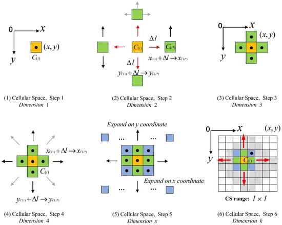
Figure 1. The modeling process of CS from the initial cellular $C_{(i)}$ by expanding $k$ dimension.

3.1.2. Modeling of the CS-IDIANA Clustering

Recommending hotel accommodation should firstly confirm the best matched tourist attractions for the tourists’ interests, which is the precondition for the tourism activities. Construct the attribute vector based on the tourist attraction cells $C_{T(i)}$ in the urban cellular space (CS), which is used to build the CS-IDIANA clustering algorithm to cluster the tourist attractions in the CS [19,20,21].

Definition 4. 

The feature attribute $p_{(i)}$ and spatial attribute $q_{(i)}$ of the tourist attraction cellular $C_{T(i)}$. The tourist attraction $T_{(i)}$ in the $C_{T(i)}$ has functional features that are different from the other attractions in the $T_{{(}^{\neg }i)}$ of the cellular $C_{T{(}^{\neg }i)}$, and the feature is defined as the feature attribute $p_{(i)}$, $0<i\le u$, $i,u\in N$. The coordinates $(x_{CT(i)},y_{CT(i)})$ of the cellular $C_{T(i)}$ in the CS coordinate system $oxy$ is the feature that distinguishes the other cellular $C_{T{(}^{\neg }i)}$, and it is defined as the spatial attribute $q_{(i)}$, $0<i\le v$, $i,v\in N$.

Definition 5. 

Attribute vector ${\zeta }_{C_{T(i)}}$ and the attribute quantification table ${\zeta }_{C_{T(i)}}$ of the tourist attraction cell $C_{T(i)}$. Construct a vector $<p_{(i)},q_{(i)}>$ to represent the cellular attributes of $C_{T(i)}$, including the feature attributes and the spatial attributes, and define this vector as the attribute vector ${\zeta }_{C_{T(i)}}$ of the $C_{T(i)}$. According to the features of the tourist attractions, each attribute is quantified into an interval range, and an attribute quantification table ${\zeta }_{C_{T(i)}}$ is constructed as Table 1. Formulas (3) and (4) show the modeling of the attribute vector ${\zeta }_{C_{T(i)}}$.

$${\zeta }_{C_{T(i)}}=⟨p_{(i)},q_{(i)}⟩$$

(3)

$${\zeta }_{C_{T(i)}}=⟨\underset{p_{(i)}}{\underbrace{\begin{array}{cccc}{p}_{(1)},& p_{(2)},& \dots ,& p_{(u)},\end{array}}}\underset{q_{(i)}}{\underbrace{\begin{array}{cccc}{q}_{(1)},& q_{(2)},& \dots ,& q_{(v)}\end{array}}}⟩$$

(4)

Table 1. The quantization table ${\zeta }_{C_{T(i)}}$ of cellular $C_{T(i)}$.

	$p_{(1)}$	$p_{(2)}$	$p_{(3)}$	$p_{(4)}$
Interval range	$0<p_{(1)}<1$	$0<p_{(2)}<1$	$0<p_{(3)}<1$	$0<p_{(4)}<1$
	$p_{(5)}$	$p_{(6)}$	$p_{(7)}$	$q_{(1)}$	$q_{(2)}$
Interval range	$\mathrm{a}: 0<p_{(5)}\le 1$; $\mathrm{b}: 1<p_{(5)}\le 3$; $\mathrm{c}: 3<p_{(5)}\le 6$; $\mathrm{d}: p_{(5)}>6$.	$\mathrm{a}: 0<p_{(6)}\le 50$; $\mathrm{b}: 50<p_{(6)}\le 100$; $\mathrm{c}: 100<p_{(6)}\le 150$; $\mathrm{d}: p_{(6)}>150$.	$0<p_{(7)}<1$	$0\le x<(k+1)·l$	$0\le y<(k+1)·l$

The symbols $p_{(1)}~p_{(4)}$ are the text attribute tags. The quantification interval is obtained according to the big data from the tourist attraction text evaluation. The symbols $p_{(5)}~p_{(7)}$ are the fixed attributes of the tourist attractions and are obtained from the official website of the tourist attractions. Specifically, $p_{(1)}$ is the natural scenery, $p_{(2)}$ is the humanistic history, $p_{(3)}$ is the leisure shopping, $p_{(4)}$ is the competitive amusement, $p_{(5)}$ is the travel time, $p_{(6)}$ is the travel fee, and $p_{(7)}$ is the TA popularity.

The symbols $q_{(1)}~q_{(2)}$ are the coordinates $(x,y)$ of the tourist attractions in the CS, namely $q_{(1)}$ is coordinate $x$, $q_{(2)}$ is coordinate $y$. The unit of the travel time $p_{(5)}$ is hours, and the unit of the travel cost $p_{(6)}$ is CNY yuan. Any cellular tourist attraction $\forall T_{(i)}$ has fixed attributes, and a cellular attribute vector ${\zeta }_{C_{T(i)}}$ is generated based on the quantization table ${\zeta }_{C_{T(i)}}$.

Definition 6. 

The clustering objective function $f({\zeta }_{C_{T(i)}},{\zeta }_{C_{T(j)}})$ of the cellular $C_{T(i)}$. The function that measures the closeness of two tourist attractions $T_{(i)}$ and $T_{(j)}$ in the cellular $C_{T(i)}$ and $C_{T(j)}$ is defined as the clustering objective function $f({\zeta }_{C_{T(i)}},{\zeta }_{C_{T(j)}})$ of the cellular $C_{T(i)}$. Based on the tourists’ interests, the feature attributes $p_{(i)}$ are extracted from the attraction attribute vector ${\zeta }_{C_{T(i)}}:<p_{(i)},q_{(i)}>$, and the objective function based on the feature attributes $p_{(i)}$ is constructed as Formula (5). To ensure that each feature attribute has the same quantitative level impact on the clustering results, the disturbance factors ${\delta }_{(i)}~p_{(i)}$ are introduced to normalize the feature attributes. In the formula, $p_{(k)}^{T(i)}$ is the No. $k$ feature attribute of the tourist attraction $T_{(i)}$, $0<k\le u$, $k,u\in N$. Calculate the average dissimilarity $\overline{f}({\zeta }_{C_{T(i)}},{\zeta }_{C_{T(j)}})$ of the tourist attractions based on the objective function $f({\zeta }_{C_{T(i)}},{\zeta }_{C_{T(j)}})$, as shown in Formula (6).

$$f({\zeta }_{C_{T(i)}},{\zeta }_{C_{T(j)}})={\left[{\displaystyle \sum _{k=1}^u{\delta }_{{(i)}^r}·{\left|p_{(k)}^{T(i)}-p_{(k)}^{T(j)}\right|}^r}\right]}^{1/r}$$

(5)

$$\overline{f}({\zeta }_{C_{T(i)}},{\zeta }_{C_{T(j)}})=\frac{{\displaystyle \sum _{j=1,i\ne j}^{m-1}f({\zeta }_{C_{T(i)}},{\zeta }_{C_{T(j)}})}}{m-1}$$

(6)

Definition 7. 

Tourist attraction cluster $C_{(i)}$. The $m$ number of tourist attractions in the CS is grouped into the $d$ number of sets with distinguished feature attributes, and the tourist attractions have the same close feature attributes in the same set, while the tourist attractions in different sets have discrepant feature attributes. The set that gathers the tourist attractions with close feature attributes is defined as the tourist attraction cluster $C_{(i)}$.The quantity of the tourist attractions in the cluster $C_{(i)}$ is $m_{(i)}$. Then, the $C_{(i)}$: $0<i\le d$, $0<m_{(i)}\le m$, $i,d,m_{(i)},m\in N$. The quantity satisfies Formula (7).

$${\displaystyle \sum _{i=1}^d{m}_{(i)}}=m$$

(7)

Definition 8. 

The clustering open list $O_p$ and closed list $C_l$. The tourist attraction which has been grouped into the arbitrary cluster $\forall C_{(i)}$ is stored in a closed list $C_l$. The tourist attraction which has not been grouped into any cluster is stored into an open list $O_p$.

According to the tourism features and clustering object, the urban CS is set as the initial cluster $C_{ini}$ to construct the clustering algorithm IDIANA. The modeling process is designed as follows (Algorithm 1). Figure 2 shows the process of generating clusters $C_{(i)}$ in the CS by using the CS-IDIANA clustering model.

Algorithm 1: CS-IDIANA clustering algorithm

Input: Cellular space (CS), $m$ number of tourist attractions $T_{(i)}$. Output:  $d$ number of clusters $C_{(i)}$, each cluster $C_{(i)}$ contains $m_{(i)}$ number of tourist attractions $T_{(i)}$. (1) $m$ number of tourist attractions $T_{(i)}$ in CS are stored into the initial cluster $C_{ini}$. The data is stored in $O_p$. (2) FOR $(i=1$, $j=1$; $i\ne j$; $i++$, $j++$) DO BEGIN (3)   Calculate the $\overline{f}({\zeta }_{C_{T(i)}},{\zeta }_{C_{T(j)}})$, $0<i,j\le u$. Confirm and select the $d$ number of $\max \overline{f}({\zeta }_{C_{T(i)}},{\zeta }_{C_{T(j)}})$. (4)   Extract $2d$ number of $T_{(i)}$ relating to the selected $\max \overline{f}({\zeta }_{C_{T(i)}},{\zeta }_{C_{T(j)}})$. (5)   DELETE the repetitive $T_{(i)}$. (6)   Choose d number of $T_{(i)}$, satisfying: the average dissimilarity $\overline{f}({\zeta }_{C_{T(i)}},{\zeta }_{C_{T(j)}})$ of $\forall T_{(i)}$ and $\forall T_{(j)}$ are all the maximum values. (7)   Deleted d number of $T_{(i)}$ in $O_p$ and store in $C_l$. d number of $T_{(i)}$ form the initial seeds for d number of clusters. (8) END FOR. (9) Recode $T_{(i)}$ in $O_p$ and $C_l$. Current $C_l$ stores $d$ number of $T_{(i)}$, code $0<i\le d$. $Op$ stores $m-d$ number of $T_{(j)}$, code $0<j\le m-d$. (10) FOR ($i=1$, $j=1$; $0<i\le d$, $0<j\le m-d$; $i++$, $j++$) DO BEGIN (11)   As to arbitrary $\forall T_{(i)}$ in $C_l$, traverse $0<j\le m-d$, take $\min {\overline{f}({\zeta }_{C_{T(i)}},{\zeta }_{C_{T(j)}})}_{(i)}$. (12)   REPEAT, calculate the $\min {\overline{f}({\zeta }_{C_{T(i)}},{\zeta }_{C_{T(j)}})}_{(i)}$, traverse $0<i\le d$. (13)   Take $\alpha =\min [\min {\overline{f}({\zeta }_{C_{T(i)}},{\zeta }_{C_{T(j)}})}_{(i)}]$, confirm code $i~T_{(i)}$, absorb $T_{(j)}$ relating to $\alpha$ into clusters $C_{(i)}$ relating to $i~T_{(i)}$. (14)   Delete $T_{(j)}$ in $O_p$, store them in $C_l$. (15)   REPEAT. When $O_p=\varnothing$ and the element quantity of $C_l$ is $m$, the searching ends. (16) END FOR. (17) Output the sub-CS relating to $C_{(i)}$, the algorithm ends.

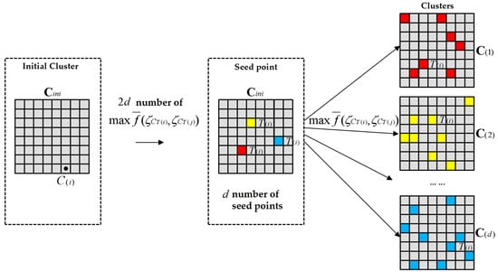
Figure 2. The process of generating clusters $C_{(i)}$ in CS using the CS-IDIANA clustering model. Different colors represent different clusters.

3.2. HAR Algorithm Based on SAFS

The necessary condition for the tourists choosing hotel accommodation is to be closest to the attractions that they will visit, aiming to reduce the travel costs. Therefore, when recommending hotel accommodation for the tourists, the first step is to search for the optimal tourist attractions, and then recommend the optimal hotels for the tourists based on their accommodation requirements [22,23]. Based on the analysis, we construct a tourist attraction SAFS model based on the urban hotels and search for the tour routes with travel costs starting from the hotels to visit all the recommended tourist attractions, according to which the hotels that generate the lowest travel costs are determined [24].

3.2.1. Tourist Attraction Searching Based on the Tourists’ Interests

Establish the tourist interest vector ${\zeta }_{user}$ and the interest quantification table ${\zeta }_{user}$ based on the attribute vector ${\zeta }_{C_{T(i)}}$ and the attribute quantification table ${\zeta }_{C_{T(i)}}$ of the tourist attraction cellular $C_{T(i)}$. Construct a vector ${\zeta }_{user}$ based on the feature attributes $p_{(i)}$ of the vector ${\zeta }_{C_{T(i)}}:<p_{(i)},q_{(i)}>$ with the elements $p_{(i)}^{user}$, $0<i\le u$, $i,u\in N$. The tourists choose the indicators from the quantification table ${\zeta }_{user}$ based on their interests, quantify and score the $u$ number of feature attributes $p_{(i)}$, and obtain the normalized vector ${\zeta }_{user}:<p_{(i)user}>$. Based on the tourist interest vector ${\zeta }_{user}$ and the feature attribute vector ${\zeta }_{C_{T(i)}}$ of each cellular $C_{T(i)}$ in each cluster $C_{(i)}$, a tourist attraction recommendation field strength model ${\mathsf{\Phi }}_{C_{T(i)}}$ is constructed as Formula (8). The recommended field strength ${\mathsf{\Phi }}_{C_{T(i)}}$ of the tourist attractions for each cluster $C_{(i)}$ represents the closeness between the tourist interest vector ${\zeta }_{user}$ and the feature attribute vector of the tourist attraction cellular $C_{T(i)}$. The higher the field strength of the tourist attraction cellular $C_{T(i)}$ is, the stronger the ability to match the tourist interest vector ${\zeta }_{user}$ will be, and the higher probability that it will be recommended. Based on the tourists’ interests in the clusters $C_{(i)}$, we search for the tourist attractions with the highest field strength ${\mathsf{\Phi }}_{C_{T(i)}}$ from each cluster $C_{(i)}$ and recommend them to the tourists, then store them in the recommendation vector $R_{C_{T(i)}}:<r_{(i)}>$.

$${\mathsf{\Phi }}_{C_{T(i)}}={\left[{\displaystyle \sum _{k=1}^u{{\delta }_{(i)}}^r·{\left|p_{(k)}^{user}-p_{(k)}^{T(i)}\right|}^r}\right]}^{-\frac{1}{r}}$$

(8)

3.2.2. The Modeling of the HAR Algorithm Based on the SAFS

The tourist attractions in the recommendation vector $R_{C_{T(i)}}:<r_{(i)}>$ are the ones that the tourists are about to visit. Set the vector $R_{C_{T(i)}}$ to contain $w$ number of tourist attractions, each of which has spatial attributes $q_{(i)}$ in the vector ${\zeta }_{C_{T(i)}}:<p_{(i)},q_{(i)}>$. There are a large number of hotels distributed in a city, and the tourists firstly provide their basic needs from the hotel accommodation, including the star level, price and popularity. Confirm the $n$ number of hotels that meet the accommodation needs from the perspective of the hotel attributes. In regard to the spatial attributes $q_{(i)}$, not all the hotels that meet the accommodation needs are spatially optimal. Thus, considering the spatial relationship and the spatial accessibility between the hotels and the tourist attractions, the hotels with the best accessibility to the tourist attractions and the lowest travel costs should be recommended. Therefore, confirming the hotel cellular $C_{H(i)}$ based on the constructed city cellular space CS and recommending hotels from the perspective of the spatial data analysis is an effective method to reduce the travel costs. In this section, we construct a HAR algorithm based on the SAFS.

In the city cellular space CS, determine the $w$ number of tourist attraction cellular $C_{T(i)}$ in the vector $R_{C_{T(i)}}$ and $n$ number of hotel cellular $C_{H(i)}$ that satisfy the tourists’ needs. The coordinates of the cellular $C_{T(i)}$ and $C_{H(i)}$ in the coordinate system $oxy$ are $(x_{CT(i)},y_{CT(i)})$ and $(X_{CH(i)},y_{CH(i)})$, respectively. According to the expansion mode of city cellular space CS, the degree of spatial obstruction between a hotel cellular $C_{H(i)}$ and a tourist attraction cellular $C_{T(i)}$ in the recommendation vector $R_{C_{T(i)}}$ is defined as the hotel spatial accessibility field strength (SAFS), noted as $\mathsf{\Phi }(C_{H(i)},C_{T(i)})$. The average value of the hotel SAFS is defined as the average spatial accessibility field strength (ASAFS), noted as $\overline{\mathsf{\Phi }}(C_{H(i)},C_{T(i)})$, which is used to measure the overall accessibility between the hotel cellular $C_{H(i)}$ and the $w$ number of tourist attraction cellular $C_{T(i)}$. According to the definition, we construct the SAFS and ASAFS as Formulas (9) and (10), in which ${\zeta }_0$ is the normalized parameter.

$$\mathsf{\Phi }(C_{H(i)},C_{T(i)})={\zeta }_0\times \frac{1}{{\left[{\left|x_{CT(i)}-x_{CH(i)}\right|}^2+{\left|y_{CT(i)}-y_{CH(i)}\right|}^2\right]}^{\frac{1}{2}}}$$

(9)

$$\overline{\mathsf{\Phi }}(C_{H(i)},C_{T(\alpha )})=\frac{{\displaystyle \sum _{\alpha =1}^w\mathsf{\Phi }(C_{H(i)},C_{T(\alpha )})}}{w}$$

(10)

From the perspective of spatial analysis, starting from the hotel $C_{H(i)}$, visiting all the $w$ number of tourist attractions in the vector $R_{C_{T(i)}}$, the whole process will form a complete tour route. Hotel $C_{H(i)}$ and attractions $C_{T(i)}$ are the nodes in the route. Due to the constraints of the urban geographical and transportation conditions, when the tourists choose certain transportation modes to travel on the route, it will cause travel costs. The lower the travel costs of the route, the higher the satisfaction of the tourists will be. When the tourists travel between these nodes, the factors that incur travel costs include the travel distance, travel time and travel fee. Among the three factors, the travel time and the travel fee are both caused by the selected transportation modes and the distances travelled on the route. Therefore, the core factor for measuring the cost of a route is the travel distance. The route that consists of the hotel $C_{H(i)}$ and $w$ number of tourist attractions $C_{T(i)}$ has $w+1$ number of nodes, which forms $w$ number of route intervals. Under the selected transportation mode ${\mathbf{t}}_{\mathbf{m}}$, the process of the tourists’ traveling from node A to node B forms a sub-interval, and the travel cost generated is determined by the travel distance. Therefore, a cost function $f_{AB}^{(i)}$ for the No. $i$ sub-interval under the transportation mode ${\mathbf{t}}_{\mathbf{m}}$ is constructed as Formula (11), in which A and B represent the adjacent nodes, and the $d_{(A,B)(i)}$ represents the travel distance of the No. $i$ sub-interval. According to the definition, the route cost function $f_{route}^{(k)}$ generated by the $w$ number of sub-intervals is constructed as Formula (12). Where $k$ represents that the current route code is No. $k$. When the number of tourist attractions is $w$, the total number of tour routes is $A(w,w)$.

$$f_{AB}^{(i)}=1-\frac{1}{d_{(A,B)(i)}}$$

(11)

$$f_{route}^{(k)}={\displaystyle \sum _{i=1}^w\left[1-\frac{1}{d_{(A,B)(i)}}\right]}$$

(12)

In the city cellular space CS, the sub-interval composed by the adjacent nodes A and B contains multiple road nodes, and the traveling distance in the sub-interval should be the shortest searching distance of the road nodes between A and B. Firstly, we determine the sub-intervals containing A and B in the city cellular space CS and, then, we determine the $k$ number of road nodes and path distances between the nodes in the sub-intervals. Construct a spatial distribution map consisting of A, B and $k$ number of road nodes, as shown in Figure 3a. Based on the urban road traffic data, we generate a directed weighted-edge graph containing A, B and road nodes, as shown in Figure 3b. In the graph, the $N_{(i)}$ is the road node within the sub-interval and the $d_{(i)}$ is the path distance between two nodes. Based on the sub-interval structure in the CS shown in Figure 3, a Simulated Huffman Encoding Tree (SHET) is established for the sub-interval in Figure 4. The parent node A in the tree represents the starting point of the sub-interval, namely a hotel. The terminal node B represents the ending tourist attraction of the sub-interval. The tree node $N_{(i)}$ is the road node between A and B. The node code $(x_{N(i)},y_{N(i)})$ represents the coordinates of the node $N_{(i)}$ in the CS, and the numerical value $d_{(p,q)}$ represents the path distance between the current node $N_{(i)}$ and the previous node $N_{(i-1)}$.

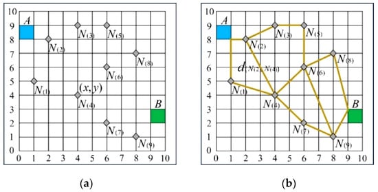
Figure 3. The constructed sub-interval and directed weighted-edge graph according to tourist attractions and road nodes. (a) shows a spatial distribution map consisting of A, B and $k$ number of road nodes. (b) shows a directed weighted-edge graph containing A, B and road nodes.

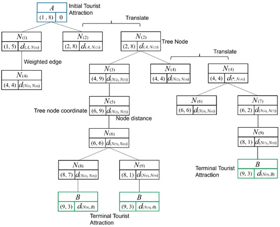
Figure 4. The constructed SHET for the sub-interval (authors’ research and computational work). In the figure, the symbol “$\ast$” in $d(\ast ,N_{(4)})$ means the two options of the former nodes $N_{(1)}$ and $N_{(2)}$. It could be $N_{(1)}$, or $N_{(2)}$.

According to the constructed SHET, we set the starting point A as $u$; $(u,v)$ is the edge of SHET, and $c_{(u,v)}$ is the edge weight. Suppose that the set $S$ stores the nodes which have confirmed the distance to the starting point $u$, while the set $T$ stores the nodes which have not confirmed the distance to the starting point $u$. The distance between the vertex $x$ in $T$ to the vertex $u$ under the current searching condition is set as $d_{(u,x)}$, and it is defined as the shortest distance starting from the vertex $u$, passing through the vertexes in $S$, and directly getting to vertex $x$, but not passing the other vertexes in $T$. The constraints are as follows: as to all the vertexes $x$ in $T$, if an edge exists between $u$ and $x$, set $d_{(u,x)}=c_{(u,x)}$, or set $d_{(u,x)}=\infty$. As to all the vertexes $x$ in $T$, find a vertex $t$ that makes $d_{(u,x)}$ the minimum one, then:

$$d_{(u,t)}=\min \left\{d_{(u,x)}\right|x\in T\}$$

(13)

In the Formula (13), the $d_{(u,t)}$ is the shortest distance between the vertex $t$ and the vertex $u$. The vertex $t$ is the node that is nearest to the vertex $u$ of all the nodes in the set $T$. Delete $t$ from $T$ and store it in $S$. As to all the vertexes $x$ that are adjacent to the vertex $t$, update the value of $d_{(u,x)}$ using Formula (14) until it gets to $T=\varnothing$.

$$d_{(u,x)}=\min \{d_{(u,x)},d_{(u,t)}+c_{(t,x)}\}$$

(14)

We design and construct the shortest path distance $d_{(A,B)(i)}$ in the sub-interval as follows:

Set the $p_{(x)}$ as the previous vertex of the vertex $x$ in the shortest path from the vertex $u$ to the vertex $x$. The $V$ is the node set containing all nodes $N_{(i)}$, vertex A and vertex B in SHET. Set $S=\left\{u\right\}$, $T=V-\left\{u\right\}$.

(1)

$\forall x\in T$, if $(u,x)\in \mathrm{SHET}$, then $d_{(u,x)}=c_{(u,x)}$, $p_{(x)}=u$; or else $d_{(u,x)}=\infty$, $p_{(x)}=-1$.

(2)

Search for $t\in T$, which makes $d_{(u,t)}=\min \left\{d_{(u,x)}\right|x\in T\}$. Then, $d_{(u,t)}$ is the shortest distance from vertex $t$ to vertex $u$.

(3)

$S=S\cup \left\{t\right\}$, $T=T-\left\{t\right\}$.

(4)

If $T=\varnothing$, the algorithm ends; or else turn to step (6).

(5)

As to all the vertexes $x$ that are adjacent to the vertex $t$, if they all satisfy $d_{(u,x)}\le d_{(u,t)}+c_{(t,x)}$, turn to step (3); or else, as to the vertexes $x$ that do not satisfy the former, set $d_{(u,x)}=d_{(u,t)}+c_{(t,x)}$, $p_{(x)}=t$, turn to step (3).

According to the hotel SAFS, the tour route cost function and the SHET algorithm for the sub-intervals, we search for the shortest path distance $d_{(A,B)(i)}$ in each sub-interval. We construct the HAR algorithm based on the SAFS as follows (Algorithm 2).

Algorithm 2: HAR algorithm based on SAFS

Input: Vector $R_{C_{T(i)}}$, $w$ number of tourist attractions $C_{T(i)}$, $n$ number of hotels $C_{H(j)}$. Output: Optimal hotel $C_{H(j)}$ with optimal spatial accessibility $\overline{\mathsf{\Phi }}(C_{H(j)},C_{T(i)})$ and route cost function $f_{route}^{(k)}$. (1) Store $w$ number of tourist attractions $C_{T(i)}$ in set ${\mathbf{C}}_{T(i)}$. Stone $n$ number of hotels $C_{H(j)}$ in set ${\mathbf{C}}_{H(j)}$. (2) FOR ($j=1$, $j=n$, $j++$) DO BEGIN (3)  FOR ($i=1$, $i=w$, $i++$) DO BEGIN (4)    Search coordinates $(x_{CT(i)},y_{CT(i)})$ and $(x_{CH(j)},y_{CH(j)})$ in the range of the CS. (5)    Calculate the $\mathsf{\Phi }(C_{H(j)},C_{T(i)})$ and $\overline{\mathsf{\Phi }}(C_{H(j)},C_{T(i)})$. (6)  END FOR (7) END FOR (8) Search for the maximum value $\max \overline{\mathsf{\Phi }}(C_{H(j)},C_{T(i)})$ in $n$ number of $\overline{\mathsf{\Phi }}(C_{H(j)},C_{T(i)})$, as well as certain suboptimal values $sub\max \overline{\mathsf{\Phi }}(C_{H(j)},C_{T(i)})$, relating to hotels $C_{H(j)}$. (9) FOR ($k=1$, $k=n$, $k++$) DO BEGIN  As for the hotels $C_{H(k)}$ and $w$ number of tourist attractions $C_{T(i)}$, search for the optimal tour route ${route}_{(k)\mathrm{opt}}$ for $C_{H(k)}$. (10)  FOR ($a=1$, $a=A(w,w)$, $a++$) DO BEGIN (11)    FOR ($v=1$, $v=w$, $v++$) DO BEGIN (12)      Search for the travel distance $d_{(A,B)(v)}$ in the No.  $v$ sub-interval of ${route}_{(a)}$. (13)      Calculate the cost $f_{AB}^{(v)}$ in the No. $v$ sub-interval of ${route}_{(a)}$. (14)    END FOR (15)    Calculate the route cost $f_{route}^{(a)}$ of the ${route}_{(a)}$. (16)  END FOR  Search for the maximum value $\max f_{route}^{(a)}$ in $A(w,w)$ number of function values $f_{route}^{(a)}$, relating to the optimal ${route}_{(k)\mathrm{opt}}$ of the $C_{H(k)}$. (17) END FOR (18) Search for the minimum value $\min f_{route}^{(k)}$ and certain sub-minimum values $sub\min f_{route}^{(k)}$ of the $n$ number of the ${route}_{(k)\mathrm{opt}}$, relating to hotels $C_{H(j)}$. (19) Judge:    ① If $\max \overline{\mathsf{\Phi }}(C_{H(j)},C_{T(i)})$ and $\min f_{route}^{(k)}$ relate to the same hotel $C_{H(j)}$, the hotel is the optimal one, the algorithm ends.    ② If $\max \overline{\mathsf{\Phi }}(C_{H(j)},C_{T(i)})$ and $\min f_{route}^{(k)}$ relate to two different hotels $C_{H(j)}$, take the one relating to the $\min f_{route}^{(k)}$ as the optimal one, the algorithm ends. (20) Output the optimal hotel $C_{H(j)}$, the algorithm ends.

4. Experiment and Result Analysis

In order to test the feasibility and the effectiveness of the proposed algorithm we design and perform an experiment, and then analyze the experimental results in regard to the aspect of clustering, the tourist attraction recommendation field strength (TA-RFS), the hotel spatial accessibility field strength (H-SAFS), the hotel recommendation result and perform a comparison on the recommendation algorithms.

4.1. Data Preparation

We take the tourism city Zhengzhou as the research object and extract 15 representative tourist attractions in Zhengzhou. The research subjects are 10 representative 4-star level hotels that can satisfy tourists’ accommodation needs. We collect the feature attributes and the spatial attributes of the tourist attractions and hotels, establish the attribute vectors and the attribute tables, and quantify all the attributes. Based on the constructed CS-IDIANA clustering algorithm, we construct the spatial cellular data for the tourist attractions and hotels, and generate the clusters throughout the cellular space. We calculate the tourist interest vector based on the tourist interest scoring data, and then calculate the TA-RFS based on the interest vector to confirm the tourist attractions for the HAR. By analyzing the hotel accommodation needs and cellular spatial relationships, we use the HAR to calculate the ASAFS and route cost of each hotel, and recommend the optimal hotel accommodation for the sample tourist. Table 2 shows the quantified tourist interest data and the hotel accommodation needs. Table 3 shows the representative tourist attractions and hotel information in Zhengzhou City, which are selected according to the tourist’s needs. In the table, TA represents tourist attraction, Ho represents hotel, and $p_{(1)}$ is: the natural scenery, $p_{(2)}$ is the humanistic history, $p_{(3)}$ is the leisure shopping, $p_{(4)}$ is: the competitive amusement, $p_{(5)}$ is: the travel time, $p_{(6)}$ is the travel fee, $p_{(7)}$ is the TA popularity, $h_{(1)}$ is the star level, $h_{(2)}$ is the price, $h_{(3)}$ is the popularity.

Table 2. The quantified tourist interest data and the hotel accommodation needs.

TA	$p_{(1)}$	$p_{(2)}$	$p_{(3)}$	$p_{(4)}$	$p_{(5)}$	$p_{(6)}$	$p_{(7)}$
Quantify value	0.90	0.50	0.20	0.10	0.20	0.50	0.60
Ho	$h_{(1)}$	$h_{(2)}$	$h_{(3)}$
Quantify range	$h_{(1)}\ge 4$	$h_{(2)}\le 500$	$h_{(3)}\ge 3.50$

Table 3. The representative tourist attractions and hotel information in Zhengzhou City.

Code	$T_{(1)}$	$T_{(2)}$	$T_{(3)}$	$T_{(4)}$	$T_{(5)}$	$T_{(6)}$	$T_{(7)}$	$T_{(8)}$
TA	Er Qi Memorial Tower	Bisha Gang Park	Century Park	Erqi Wanda	Henan Museum	Zhong Yuan Wanda	De Hua Street	The People’s Park
Code	$T_{(9)}$	$T_{(10)}$	$T_{(11)}$	$T_{(12)}$	$T_{(13)}$	$T_{(14)}$	$T_{(15)}$
TA	Zheng Zhou Zoo	Zheng Zhou Museum	Long Hu Park	Zi Jing Shan Park	Xi Liu Lake	Early-Shang Dynasty Site	Guo Mao
Code	$H_{(1)}$	$H_{(2)}$	$H_{(3)}$	$H_{(4)}$	$H_{(5)}$
Ho	Song Shan Hotel	Zhongdu Hotel	HongRun HuaXia Hotel	Da He Jin Jiang Hotel	Wei Lai Hotel
Code	$H_{(6)}$	$H_{(7)}$	$H_{(8)}$	$H_{(9)}$	$H_{(10)}$
Ho	Tian Di Yue Hai Hotel	Jin Qiao Hotel	Rebecca Hotel	Da He International Hotel	Yingcheng Xindi Hotel

4.2. Clustering Results

We use the constructed CS-IDIANA to generate the clusters on the 15 selected tourist attractions and calculate the average dissimilarity $\overline{f}({\zeta }_{C_{T(i)}},{\zeta }_{C_{T(j)}})$ of the tourist attractions, as shown in Table 4. This is combined with the clustering objective function values $f({\zeta }_{C_{T(i)}},{\zeta }_{C_{T(j)}})$ between the initial seed attraction of the cluster and the other attractions; the cellular space of each cluster is generated as shown in Figure 5. The cellular spaces (a)–(c) represent the clustering $C_{\left(1\right)}$–$C_{\left(3\right)}$, whose codes are the numbers of the tourist attraction cellular $C_{T(i)}$. The cellular space (d) is the hotel cellular $C_{H(i)}$, whose code is the number of the hotel cellular $C_{H(i)}$. The average dissimilarity is arranged in descending order (with the tourist attraction numbers in parentheses) as follows: 0.9193 (4 and 6), 0.9103 (5), 0.9098 (15), 0.8746 (7), 0.8724 (10), 0.8583 (1), 0.8336 (14), 0.8028 (13), 0.7827 (2), 0.7461 (9), 0.7349 (8), 0.7308 (12), 0.7292 (11), 0.6746 (3).

Table 4. The average dissimilarity $\overline{f}({\zeta }_{C_{T(i)}},{\zeta }_{C_{T(j)}})$ of the tourist attractions.

TA	$T_{(1)}$	$T_{(2)}$	$T_{(3)}$	$T_{(4)}$	$T_{(5)}$	$T_{(6)}$	$T_{(7)}$	$T_{(8)}$
$\overline{f}({\zeta }_{C_{T(i)}},{\zeta }_{C_{T(j)}})$	0.8583	0.7827	0.6746	0.9193	0.9103	0.9193	0.8746	0.7349
TA	$T_{(9)}$	$T_{(10)}$	$T_{(11)}$	$T_{(12)}$	$T_{(13)}$	$T_{(14)}$	$T_{(15)}$
$\overline{f}({\zeta }_{C_{T(i)}},{\zeta }_{C_{T(j)}})$	0.7461	0.8724	0.7292	0.7308	0.8028	0.8336	0.9098

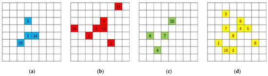
Figure 5. Cluster cellular space ($\mathrm{CS}-C_{(i)}$) and hotel cellular space ($\mathrm{CS}-H_{(i)}$) (authors’ research and computational work). (a) Cluster $C_{(1)}$; (b) cluster $C_{(2)}$; (c) cluster $C_{(3)}$; (d) hotel cellular.

Analyze the data in Table 4 and Figure 5. The initial seed point of each cluster is selected from the tourist attractions with the highest average dissimilarity. Then, combining it with the clustering objective function values of the seed point with the other tourist attractions, the closeness between the seed point and the other tourist attractions are determined. The attractions with the highest average dissimilarity are $T_{(4)}$ and $T_{(6)}$, with the objective function value of 0, and are grouped into the same cluster. $T_{(4)}$ is selected as the seed point to generate the cluster. The tourist attraction with the second highest average dissimilarity is $T_{(5)}$, and the clustering objective function values between $T_{(5)}$–$T_{(4)}$, $T_{(5)}$–$T_{(6)}$ are 1.1395 and 1.1395, which are much higher than those of the other tourist attractions. Thus, $T_{(5)}$ belongs to a different cluster, rather than the cluster of $T_{(4)}$. Set $T_{(5)}$ as the seed point for another new cluster. The third highest average dissimilarity is $T_{(15)}$, and the clustering objective function values between $T_{(15)}$–$T_{(4)}$, $T_{(15)}$–$T_{(6)}$ are 0.2245 and 0.2245, which are much smaller than those of the other tourist attractions. Therefore, the closeness between $T_{(15)}$ and $T_{(4)}$, $T_{(6)}$ is very high, and $T_{(15)}$ is grouped into the cluster of $T_{(4)}$. In the same way, judge that the average dissimilarity of $T_{(13)}$ is the maximum value 0.8028, and the clustering objective function values between $T_{(13)}$–$T_{(4)}$, $T_{(13)}$–$T_{(5)}$ are 1.2828 and 1.1285, indicating a low closeness between $T_{(13)}$ and $T_{(4)}$, $T_{(5)}$. Thus, set $T_{(13)}$ as the seed point for another new cluster. As for the CS-IDIANA clustering algorithm, the 15 tourist attractions are finally grouped into three clusters.

4.3. TA-RFS Results

Based on the tourists’ data in Table 2, we calculate the TA-RFS of ${\mathsf{\Phi }}_{C_{T(i)}}$ for the tourist attractions in each cluster, as shown in Table 5. Output the 3D peak plot of the TA-RFS of ${\mathsf{\Phi }}_{C_{T(i)}}$ for each cluster in the CS coordinate system, as shown in Figure 6.

Table 5. The TA-RFS of ${\mathsf{\Phi }}_{C_{T(i)}}$ for tourist attractions in each cluster.

Cluster $C_{(1)}$	$T_{(1)}$	$T_{(5)}$	$T_{(10)}$	$T_{(14)}$
${\mathsf{\Phi }}_{C_{T(i)}}$	0.8939	0.8924	0.9098	1.0008
Cluster $C_{(2)}$	$T_{(2)}$	$T_{(3)}$	$T_{(8)}$	$T_{(9)}$	$T_{(11)}$	$T_{(12)}$	$T_{(13)}$
${\mathsf{\Phi }}_{C_{T(i)}}$	1.3834	1.4655	1.6509	2.3564	1.4866	1.7178	1.5278
Cluster $C_{(3)}$	$T_{(4)}$	$T_{(6)}$	$T_{(7)}$	$T_{(15)}$
${\mathsf{\Phi }}_{C_{T(i)}}$	0.7324	0.7324	0.7683	0.7539

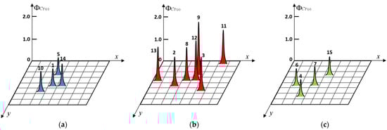
Figure 6. The 3D peak plot of the TA-RFS of ${\mathsf{\Phi }}_{C_{T(i)}}$ for each cluster in CS coordinate system (authors’ research and computational work). (a) Cluster $C_{(1)}$; (b) cluster $C_{(2)}$; (c) cluster $C_{(3)}$.

Analyze Table 5 and Figure 6. It can be concluded that the highest TA-RFS in the cluster $C_{(1)}$, $C_{(2)}$ and $C_{(3)}$ are 1.0008, 2.3564 and 0.7683, relating to the tourist attractions $T_{(14)}$, $T_{(9)}$ and $T_{(7)}$. The smallest TA-RFS in the cluster $C_{(1)}$, $C_{(2)}$ and $C_{(3)}$ are 0.8924, 1.3834 and 0.7324, relating to the tourist attractions $T_{(5)}$, $T_{(2)}$, $T_{(4)}$ and $T_{(6)}$. When the tourist confirms the clusters of interest, the recommendation system will provide the tourist with the tourist attractions in the sequence of descending TA-RFS. In the experiment, we set that the sample tourist prefers the tourist attractions of cluster $C_{(1)}$, the humanistic history cluster, and $C_{(2)}$, the natural scenery cluster, and has no interests in $C_{(3)}$, the leisure shopping. In a one-day tour, the tourist wishes to visit three tourist attractions, including two tourist attractions in $C_{(1)}$, the humanistic history cluster, and one tourist attraction in $C_{(2)}$, the natural scenery cluster. Based on the requirements, the recommended tourist attractions are $T_{(9)}$, $T_{(10)}$ and $T_{(14)}$.

4.4. H-SAFS and Hotel Recommendation Results

Based on the tourist attractions $T_{(9)}$, $T_{(10)}$ and $T_{(14)}$, we calculate the ASAFS of each hotel in the cellular space CS, the route cost function value starting from each hotel and the corresponding order of the route function values. Suppose that the sample tourist chooses the transportation method ${\mathbf{t}}_{\mathbf{m}}$-taxi. Table 6 shows the results of the SAFS and the ASAFS on each hotel to the recommended tourist attractions. The data results are visualized in Figure 7. Figure 7a–c shows the trend in the SAFS on the tourist attractions $T_{(9)}$, $T_{(10)}$ and $T_{(14)}$ to the hotels, and Figure 7d shows the trend in the ASAFS on each hotel. Table 7 shows the comparison of the SAFS and the ASAFS between the hotel with the highest ASAFS and the two hotels with the second highest ASAFS. Table 8 shows the minimum value (optimal) and two sub-minimum values (suboptimal) of the route cost function starting from each hotel, along with their corresponding routes. Route 1 represents the optimal route, while Route 2 and Route 3 represent the suboptimal routes. Figure 8a–c shows the cost trend chart of the optimal, the suboptimal and the third optimal routes corresponding to the hotels. Figure 8a shows the trend in the cost function value of the optimal route corresponding to each hotel, noted by the red curve. Figure 8b shows the trend of the cost function value of the suboptimal route corresponding to each hotel, noted by the blue curve. Figure 8c shows the trend in the cost function value of the third optimal route corresponding to each hotel, noted by the green curve. Figure 8d shows the comparison on the SAFS and the ASAFS between the optimal hotel and the suboptimal hotels. The blue bars represent the differences in the SAFS and the ASAFS between the hotels $H_{(1)}$ and $H_{(8)}$. The orange bars represent the differences in the SAFS and the ASAFS between the hotels $H_{(1)}$ and $H_{(14)}$.

Table 6. The results of the SAFS and the ASAFS on each hotel to the recommended tourist attractions.

Ho		$\mathbf{ASAFS}\mathbf{\Phi }$		$\mathbf{ASAFS}\overline{\mathbf{\Phi }}$
	${\mathit{T}}_{(9)}$	${\mathit{T}}_{(10)}$	${\mathit{T}}_{(14)}$
$H_{(1)}$	0.1299	1.4265	0.1695	0.5753
$H_{(2)}$	0.1235	0.2778	0.2326	0.2113
$H_{(3)}$	0.1961	0.1493	0.1205	0.1553
$H_{(4)}$	0.5556	0.1724	0.3333	0.3538
$H_{(5)}$	0.3448	0.1282	0.3125	0.2618
$H_{(6)}$	0.7692	0.1282	0.2222	0.3732
$H_{(7)}$	0.2564	0.3226	0.2564	0.2785
$H_{(8)}$	0.2273	0.2222	0.8333	0.4276
$H_{(9)}$	0.1176	0.0901	0.1786	0.1288
$H_{(10)}$	0.1235	0.3571	0.2128	0.2311

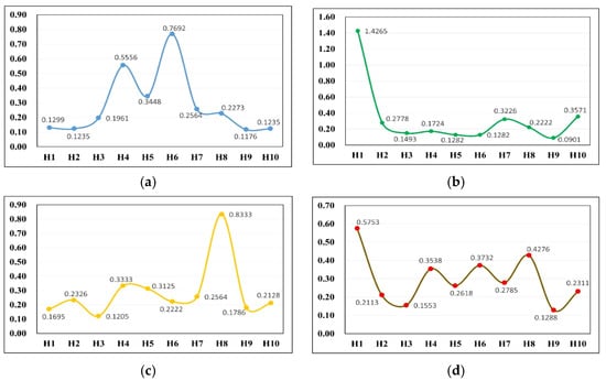
Figure 7. The trend curves for the SAFS and ASAFS on each hotel to the recommended tourist attractions (authors’ research and computational work). (a) Tourist attraction $T_{(9)}$; (b) tourist attraction $T_{(10)}$; (c) tourist attraction $T_{(14)}$; (d) ASAFS $\overline{\mathsf{\Phi }}$.

Table 7. The comparison of the SAFS and the ASAFS between the hotel with the highest ASAFS and the two hotels with the second highest ASAFS.

Ho	$\mathbf{\Delta }\mathbf{\Phi }$						$\overline{\mathbf{\Phi }}$	$\mathbf{\Delta }\overline{\mathbf{\Phi }}$
	${\mathit{T}}_{(9)}$	${\mathit{T}}_{(9)}$	${\mathit{T}}_{(10)}$	${\mathit{T}}_{(10)}$	${\mathit{T}}_{(14)}$	${\mathit{T}}_{(14)}$
$H_{(1)}$	0.1299		1.4265		0.1695		0.5753
$H_{(8)}$	0.2273	−0.0974	0.2222	1.2043	0.8333	−0.6638	0.4276	0.1477
$H_{(6)}$	0.7692	−0.6393	0.1282	1.2983	0.2222	−0.0527	0.3732	0.2021

Table 8. The minimum value (optimal) and two sub-minimum values (suboptimal) of the route cost function starting from each hotel, along with their corresponding routes.

Ho	Route 1	Route 2	Route 3	${\mathit{f}}_{\mathit{r}\mathit{o}\mathit{u}\mathit{t}\mathit{e}}^{(1)}$	${\mathit{f}}_{\mathit{r}\mathit{o}\mathit{u}\mathit{t}\mathit{e}}^{(2)}$	${\mathit{f}}_{\mathit{r}\mathit{o}\mathit{u}\mathit{t}\mathit{e}}^{(3)}$
$H_{(1)}$	$H_{(1)}{T}_{(10)}{T}_{(14)}{T}_{(9)}$	$H_{(1)}{T}_{(10)}{T}_{(9)}{T}_{(14)}$	$H_{(1)}{T}_{(9)}{T}_{(14)}{T}_{(10)}$	2.1175	2.1626	2.5710
$H_{(2)}$	$H_{(2)}{T}_{(10)}{T}_{(14)}{T}_{(9)}$	$H_{(2)}{T}_{(10)}{T}_{(9)}{T}_{(14)}$	$H_{(2)}{T}_{(14)}{T}_{(9)}{T}_{(10)}$	2.4879	2.5330	2.5689
$H_{(3)}$	$H_{(3)}{T}_{(9)}{T}_{(14)}{T}_{(10)}$	$H_{(3)}{T}_{(10)}{T}_{(14)}{T}_{(9)}$	$H_{(3)}{T}_{(9)}{T}_{(10)}{T}_{(14)}$	2.5215	2.5526	2.5906
$H_{(4)}$	$H_{(4)}{T}_{(9)}{T}_{(14)}{T}_{(10)}$	$H_{(4)}{T}_{(9)}{T}_{(10)}{T}_{(14)}$	$H_{(4)}{T}_{(14)}{T}_{(9)}{T}_{(10)}$	2.2185	2.2876	2.4241
$H_{(5)}$	$H_{(5)}{T}_{(9)}{T}_{(14)}{T}_{(10)}$	$H_{(5)}{T}_{(14)}{T}_{(9)}{T}_{(10)}$	$H_{(5)}{T}_{(9)}{T}_{(10)}{T}_{(14)}$	2.4603	2.5259	2.5293
$H_{(6)}$	$H_{(6)}{T}_{(9)}{T}_{(14)}{T}_{(10)}$	$H_{(6)}{T}_{(9)}{T}_{(10)}{T}_{(14)}$	$H_{(6)}{T}_{(14)}{T}_{(9)}{T}_{(10)}$	2.1969	2.2659	2.5458
$H_{(7)}$	$H_{(7)}{T}_{(10)}{T}_{(14)}{T}_{(9)}$	$H_{(7)}{T}_{(10)}{T}_{(9)}{T}_{(14)}$	$H_{(7)}{T}_{(9)}{T}_{(14)}{T}_{(10)}$	2.4230	2.4682	2.5302
$H_{(8)}$	$H_{(8)}{T}_{(14)}{T}_{(9)}{T}_{(10)}$	$H_{(8)}{T}_{(14)}{T}_{(10)}{T}_{(9)}$	$H_{(8)}{T}_{(10)}{T}_{(14)}{T}_{(9)}$	2.0039	2.0278	2.4770
$H_{(9)}$	$H_{(9)}{T}_{(9)}{T}_{(14)}{T}_{(10)}$	$H_{(9)}{T}_{(14)}{T}_{(9)}{T}_{(10)}$	$H_{(9)}{T}_{(10)}{T}_{(14)}{T}_{(9)}$	2.5897	2.5962	2.5990
$H_{(10)}$	$H_{(10)}{T}_{(10)}{T}_{(14)}{T}_{(9)}$	$H_{(10)}{T}_{(10)}{T}_{(9)}{T}_{(14)}$	$H_{(10)}{T}_{(14)}{T}_{(9)}{T}_{(10)}$	2.4458	2.4909	2.5689

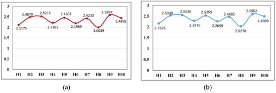
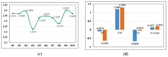
Figure 8. The trend curves for the route cost function values for each hotel and the comparison on the SAFS and ASAFS (authors’ research and computational work). (a) shows the trend in the cost function value of the optimal route corresponding to each hotel, noted by the red curve. (b) shows the trend of the cost function value of the suboptimal route corresponding to each hotel, noted by the blue curve. (c) shows the trend in the cost function value of the third optimal route corresponding to each hotel, noted by the green curve. (d) shows the comparison on the SAFS and the ASAFS between the optimal hotel and the suboptimal hotels.

Analyze the results in Table 6 and Figure 7. The same hotel has different SAFS for different tourist attractions, and the same tourist attraction also has different SAFS for each hotel. Among them, for the tourist attraction $T_{(9)}$, the SAFS of hotel $H_{(6)}$ reaches the highest value 0.7692; for the tourist attraction $T_{(10)}$, the SAFS of hotel $H_{(1)}$ reaches the highest value 1.4265; for the tourist attraction $T_{(14)}$, the SAFS of hotel $H_{(8)}$ reaches the highest value 0.8333. Among all the hotels, the ASAFS of hotel $H_{(1)}$ is the highest, at 0.5753, followed by hotel $H_{(8)}$, with the ASAFS of 0.4276; then the smallest one is hotel $H_{(6)}$, with the ASAFS of 0.3732. From Figure 5, it can be concluded that the SAFS and the ASAFS of each hotel corresponding to the tourist attractions, show a fluctuating trend, indicating that due to the constraints of the urban geographical conditions, the spatial accessibility of each hotel has significant differences, which will cause significant differences in the travel costs. When analyzing the results in Table 7 and Figure 8d, and comparing hotel $H_{(1)}$ with the optimal SAFS and the hotels $H_{(6)}$ and $H_{(8)}$ with the suboptimal SAFS, it is concluded that for the tourist attraction $T_{(9)}$, the SAFS differences are −0.0974 and −0.6393; while for the tourist attraction $T_{(10)}$, the SAFS differences are 1.2043 and 1.2983; for the tourist attraction $T_{(14)}$, the SAFS differences are −0.6638 and −0.0527. When comparing the ASAFS of the optimal hotel $H_{(1)}$ to the sub-optimal hotels $H_{(6)}$ and $H_{(8)}$, the differences are 0.1477 and 0.2021. The results show that though the ASAFS of the hotel $H_{(1)}$ is higher than that of the hotels $H_{(6)}$ and $H_{(8)}$, at the tourist attractions $T_{(9)}$ and $T_{(14)}$, its SAFS is smaller than that of the hotels $H_{(6)}$ and $H_{(8)}$. The hotel $H_{(1)}$ has an advantage in regard to the ASAFS.

Analyze the results in Table 8 and Figure 8a–c. The route cost function values for each hotel’s optimal route, suboptimal route and the third optimal route show a fluctuating trend. In regard to the optimal routes, the hotel corresponding to the smallest route cost function value is $H_{(8)}$, followed by the hotels $H_{(1)}$ and $H_{(6)}$. In regard to the suboptimal routes, the hotel corresponding to the smallest route cost function value is $H_{(8)}$, followed by the hotels $H_{(1)}$ and $H_{(6)}$. In regard to the third optimal routes, the hotel corresponding to the smallest route cost function value is $H_{(4)}$, followed by the hotels $H_{(8)}$ and $H_{(5)}$. It can be concluded that the optimal route has the lowest function cost, and it will cause the lowest travel costs.

(1)

In all the optimal routes, the route $H_{(8)}{T}_{(14)}{T}_{(9)}{T}_{(10)}$ of hotel $H_{(8)}$ has the smallest cost function value 2.0039, followed by the route $H_{(1)}{T}_{(10)}{T}_{(14)}{T}_{(9)}$ of hotel $H_{(1)}$ and the route $H_{(6)}{T}_{(9)}{T}_{(14)}{T}_{(10)}$ of hotel $H_{(6)}$, the cost function values are 2.1175 and 2.1969. Thus, compared with the hotels $H_{(1)}$ and $H_{(6)}$, hotel $H_{(8)}$ can reduce the travel costs by 5.67% and 9.63%; compared to hotel $H_{(9)}$ with the highest route cost, hotel $H_{(1)}$ reduces the travel costs by 29.23%.

(2)

In all the suboptimal routes, the route $H_{(8)}{T}_{(14)}{T}_{(10)}{T}_{(9)}$ of hotel $H_{(8)}$ has the smallest cost function value 2.0278, followed by the route $H_{(1)}{T}_{(10)}{T}_{(9)}{T}_{(14)}$ of hotel $H_{(1)}$ and the route $H_{(6)}{T}_{(9)}{T}_{(10)}{T}_{(14)}$ of hotel $H_{(6)}$, the cost function values are 2.1626 and 2.2659. Thus, compared with the hotels $H_{(1)}$ and $H_{(6)}$, hotel $H_{(8)}$ can reduce the travel costs by 6.65% and 11.74%; compared to hotel $H_{(9)}$ with the highest route cost, hotel $H_{(1)}$ reduces the travel costs by 28.03%.

(3)

In all the third optimal routes, the route $H_{(4)}{T}_{(14)}{T}_{(9)}{T}_{(10)}$ of hotel $H_{(4)}$ has the smallest cost function value 2.4241, followed by the route $H_{(8)}{T}_{(10)}{T}_{(14)}{T}_{(9)}$ of hotel $H_{(8)}$ and the route $H_{(5)}{T}_{(9)}{T}_{(10)}{T}_{(14)}$ of hotel $H_{(5)}$, the cost function values are 2.4770 and 2.5293. Thus, compared with the hotels $H_{(8)}$ and $H_{(5)}$, hotel $H_{(4)}$ can reduce the travel costs by 2.18% and 4.34%; compared to hotel $H_{(9)}$ with the highest route cost, hotel $H_{(4)}$ reduces the travel costs by 7.22%.

By analyzing the results, it can be concluded that, under the recommended tourist attractions $T_{(9)}$, $T_{(10)}$ and $T_{(14)}$, the route corresponding to hotel $H_{(8)}$ has the smallest cost function value, and it is the optimal recommended hotel. If the tourist travels on route $H_{(8)}{T}_{(14)}{T}_{(9)}{T}_{(10)}$, the travel costs will be the lowest, followed by the hotels $H_{(1)}$ and $H_{(6)}$. The experiment verifies that the proposed algorithm can search and find the optimal hotel accommodation with the optimal spatial accessibility and the lowest travel costs. The recommended hotel can meet the tourists’ accommodation needs and reduce the route travel costs to the lowest amount.

4.5. Comparison on Recommendation Algorithms

The accuracy, recall rate, precision and F₁ value are the indexes used to test the effectiveness of a recommendation algorithm. Accuracy measures the ability of a system to judge the right items and the wrong items. In a recommendation system, accuracy means the ratio of the accurate judgement items both on the recommended and not recommended items to the total quantity of the judgement items. The recall rate measures the ability of a system to judge the right items from the total number of right and wrong items. In a recommendation system, the recall rate means the ratio of the final recommended items to the total number of items that should be actually recommended. The precision measures the ability of the recommendation algorithm to judge the right items that should be recommended from the total number of items actually recommended. It equates to the ratio of the right items that should be recommended to the total number of items actually recommended. Precision and recall are the two factors used to calculate the F₁ value. The F₁ metric unifies the precision and recall into one metric standard, which is the harmonic mean of the precision and the recall. It not only reflects the precision of the algorithm model, but also better reflects the completeness of the algorithm model. The higher the F₁ value of the recommendation algorithm, the better the performance of the recommendation algorithm will be, and the recommendation results will better match the users’ demands.

Formula (15) is the calculation method for evaluating the accuracy of recommendation algorithms. Formula (16) is the calculation method for evaluating the recall rate of recommendation algorithms, in which $TP$ represents the quantity of the hotels that should be recommended and finally successfully recommended, $TN$ represents the quantity of the hotels that should not be recommended and finally not recommended, $FP$ represents the quantity of the hotels that should not be recommended but finally recommended, and $FN$ represents the quantity of the hotels that should be recommended but finally fail to be recommended. Formula (17) is the calculation method for evaluating the precision of recommendation algorithms, which is a critical factor to calculate the F₁ value. Formula (18) is the model of the F₁ metric for the recommendation algorithm.

$$\mathrm{Accuracy}=\frac{TP+TN}{TP+TN+FP+FN}$$

(15)

$$\mathrm{Recall}=\frac{TP}{TP+FN}$$

(16)

$$\mathrm{Precision}=\frac{TP}{TP+FP}$$

(17)

$$F_1=\frac{2·\mathrm{Precision}·\mathrm{Recall}}{\mathrm{Precision}+\mathrm{Recall}}$$

(18)

In this experiment, we used $TP$, $FP$, $TN$ and $FN$ as four indicators to calculate the accuracy and recall of the recommendation algorithm. The measurement methods for these four indicators are as follows:

• $TP$: In all the hotel samples, $TP$ is the number of hotels that should be recommended to the sample tourist and ultimately recommended to the sample tourist. It represents the correct recommendation result.
• $FP$: In all the hotel samples, $FP$ is the number of hotels that should not be recommended to the sample tourist, but ultimately recommended to the sample tourist. It represents the wrong recommendation result.
• $TN$: In all the hotel samples, $TN$ is the number of hotels that should not be recommended to the sample tourist and ultimately not recommended to the sample tourist. It represents the correct recommendation result.
• $FN$: In all the hotel samples, $FN$ is the number of hotels that should be recommended to the sample tourist, but ultimately not recommended to the sample tourist. It represents the wrong recommendation result.

In recommending the hotels, we use the recommendation algorithms to calculate and output a certain quantity of hotels and provide them to the sample tourist. If the output hotels satisfy the tourist’s interests, or have the optimal spatial accessibility and route cost, they could be supposed as the hotels that should be recommended. In the total recommended hotels and the hotels that are not recommended, we judge them as the ones belonging to $TP$, $FP$, $TN$ or $FN$, respectively, and then calculate the accuracy, recall rate, precision and F₁ value.

We select the two commonly used recommendation algorithms: the user-based collaborative filtering recommendation (UCFR) and the item-based collaborative filtering recommendation (ICFR) as the control group. The experimental group uses the proposed recommendation method based on the CS-IDIANA clustering algorithm (CSIDR). The experimental conditions are set as shown in Table 2. The hotel accommodation requirements are set as follows: $h_{(1)}$ is the star level constraint, $h_{(1)}\ge 4$; $h_{(2)}$ is the price constraint, $h_{(2)}\le 500.00$; $h_{(3)}$ is the popularity constraint, $h_{(3)}\ge 3.50$. For the control group UCFR, we search for users with similar accommodation needs as the sample tourist. We select 1250 pieces of information from the user evaluations on the sample hotels in Table 3 from the official website of “DaZhongDianPing” (https://www.dianping.com/), and use the text mining method to extract the keywords and perform the word frequency statistics on the comment data, and cluster the evaluation users based on the comment data. By calculating the closeness between the clustering features and the sample tourist features, as well as the frequency of the hotel matching, the UCFR recommends the users and their corresponding hotels in the cluster with the highest matching degree for the sample tourist. For the control group ICFR, we search for the hotel that best matches the accommodation needs of the sample tourist. We search for and quantify the feature attributes of the sample hotels in Table 3 from the official website of “DaZhongDianPing”, and construct a matching function between the feature attributes of the sample tourist and the hotels and calculate their closeness, then recommend the hotels to the tourists based on the closeness ranking. According to the hotel accommodation standards in this paper, we select the number of hotels $k=5$, $k=6$, $k=7$, $k=8$ with the optimal ASAFS and route cost function as the recommended standard, while the other hotels are not recommended. Recommend four optimal hotels by using the UCFR, ICFR and CSIDR, and calculate the accuracy, recall, precision and F₁ of each algorithm based on the travel cost. The results are shown in Table 9. Based on Table 9, we obtain the comparison chart on the accuracy, recall rate, precision and F₁ value of each algorithm for the optimal number of hotels $k=5$, $k=6$, $k=7$, $k=8$, as shown in Figure 9. Figure 9a–c shows a comparison of the accuracy, recall rate and precision of each algorithm under the condition of the ASAFS, and Figure 9d–f shows a comparison of the accuracy, recall rate and precision of each algorithm under the condition of the route cost function. Figure 10 shows a comparison on the F₁ of each algorithm under the condition of the ASAFS and the route cost, in which Figure 10a represents the ASAFS condition and Figure 10b represents the route cost condition. In Figure 9 and Figure 10, the blue, orange and gray data represent the CSIDR, UCFR and ICFR.

Table 9. The comparison on the accuracy, recall rate, precision and F₁ value of each algorithm based on the ASAFS of $\overline{\mathsf{\Phi }}$ and route cost function $f_{route}^{(k)}$.

$\overline{\mathbf{\Phi }}$		$\mathit{k}=5$	$\mathit{k}=6$	$\mathit{k}=7$	$\mathit{k}=8$	${\mathit{f}}_{\mathit{r}\mathit{o}\mathit{u}\mathit{t}\mathit{e}}^{(\mathit{k})}$		$\mathit{k}=5$	$\mathit{k}=6$	$\mathit{k}=7$	$\mathit{k}=8$
Accuracy	CSIDR	0.9000	0.8000	0.7000	0.6000	Accuracy	CSIDR	0.9000	0.8000	0.7000	0.6000
	UCFR	0.5000	0.4000	0.3000	0.2000		UCFR	0.5000	0.4000	0.3000	0.2000
	ICFR	0.8000	0.7000	0.6000	0.5000		ICFR	0.8000	0.7000	0.6000	0.5000
Recall	CSIDR	0.8000	0.6667	0.5714	0.5000	Recall	CSIDR	0.8000	0.6667	0.5714	0.5000
	UCFR	0.4000	0.3333	0.2857	0.2500		UCFR	0.4000	0.3333	0.2857	0.2500
	ICFR	0.6000	0.5000	0.4286	0.3750		ICFR	0.6000	0.5000	0.4286	0.3750
Precision	CSIDR	1.0000	1.0000	1.0000	1.0000	Precision	CSIDR	1.0000	1.0000	1.0000	1.0000
	UCFR	0.5000	0.5000	0.5000	0.5000		UCFR	0.5000	0.5000	0.5000	0.5000
	ICFR	1.0000	1.0000	1.0000	1.0000		ICFR	1.0000	1.0000	1.0000	1.0000
F1	CSIDR	0.8889	0.8000	0.7272	0.6667	F1	CSIDR	0.8889	0.8000	0.7272	0.6667
	UCFR	0.4444	0.4000	0.3636	0.3333		UCFR	0.4444	0.4000	0.3636	0.3333
	ICFR	0.7500	0.6667	0.6000	0.5455		ICFR	0.7500	0.6667	0.6000	0.5455

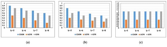
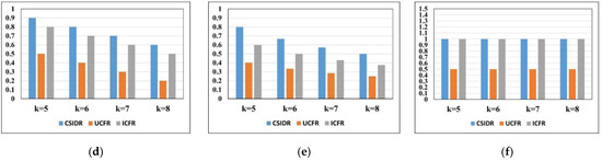
Figure 9. The comparison charts on the accuracy, recall rate, precision of each algorithm based on the ASAFS of $\overline{\mathsf{\Phi }}$ and the route cost function $f_{route}^{(k)}$ (authors’ research and computational work). (a) Accuracy; (b) recall rate; (c) precision; (d) accuracy; (e) recall rate; (f) precision.

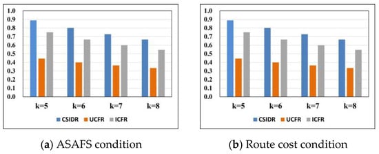
Figure 10. The comparison on the F₁ of each algorithm under the condition of the ASAFS and the route cost. (a) Represents the ASAFS condition, and (b) represents the route cost condition (authors’ research and computational work).

Firstly, after analyzing the results in Table 9 and Figure 9, it can be concluded that:

(1) Under the constraint of the ASAFS, the CSIDR has a higher accuracy rate than the UCFR and ICFR at $k=5$, $k=6$, $k=7$, $k=8$, indicating that the hotels recommended by the CSIDR have higher accuracy rates than the UCFR and ICFR in regard to the aspect of the ASAFS, which can recommend more hotels with the maximum SAFS than the UCFR and ICFR, and it has the best algorithm performance. The ICFR has a higher accuracy rate than the UCFR at $k=5$, $k=6$, $k=7$, $k=8$, indicating that the hotels recommended by the ICFR have higher accuracy rates than the UCFR in regard to the aspect of the ASAFS, which can recommend more hotels with the maximum SAFS than the UCFR, and it has better algorithm performance than the UCFR.

The CSIDR has a higher recall rate than the UCFR and ICFR at $k=5$, $k=6$, $k=7$, $k=8$, indicating that the ratio of the CSIDR achieving the hotel recommendations with the optimal ASAFS, among all the recommended hotels, is higher than that of the UCFR and ICFR, and it has the best algorithm performance. The ICFR has higher recall rate than the UCFR at $k=5$, $k=6$, $k=7$, $k=8$, indicating that the ratio of the ICFR achieving the hotel recommendations with the optimal ASAFS, among all the recommended hotels, is higher than that of the UCFR, and it has better algorithm performance.

The CSIDR has higher precision than the UCFR and has the equivalent precision to the ICFR at $k=5$, $k=6$, $k=7$, $k=8$, indicating that the capacity of the CSIDR in achieving the right hotels that should be recommended with the optimal ASAFS, among all the hotels having been recommended, is higher than that of the UCFR, which is equivalent to the ICFR, thus it has the best performance, especially in regard to the aspect of the individual class on recommending the right items.

(2) Under the constraint of the route cost function, the CSIDR has a higher accuracy rate than the UCFR and ICFR at $k=5$, $k=6$, $k=7$, $k=8$, indicating that the hotels recommended by the CSIDR have higher accuracy rates than the UCFR and ICFR in regard to the aspect of the route travel costs, which can recommend more hotels with the minimum travel costs than the UCFR and ICFR, and it has the best algorithm performance. The ICFR has a higher accuracy rate than the UCFR at $k=5$, $k=6$, $k=7$, $k=8$, indicating that the hotels recommended by the ICFR have higher accuracy rates than the UCFR in regard to the aspect of the route travel costs, which can recommend more hotels with the minimum route travel costs than the UCFR, and it has better algorithm performance than the UCFR.

The CSIDR has a higher recall rate than the UCFR and ICFR at $k=5$, $k=6$, $k=7$, $k=8$, indicating that the ratio of the CSIDR achieving the hotel recommendations with the minimum route travel costs, among all the recommended hotels, is higher than that of the UCFR and ICFR, and it has the best algorithm performance. The ICFR has a higher recall rate than the UCFR at $k=5$, $k=6$, $k=7$, $k=8$, indicating that the ratio of the ICFR achieving the hotel recommendations with the minimum route travel costs, among all the recommended hotels, is higher than that of the UCFR, and it has better algorithm performance.

The CSIDR has higher precision than the UCFR and has the equivalent precision to the ICFR at $k=5$, $k=6$, $k=7$, $k=8$, indicating that the capacity of the CSIDR in achieving the right hotels that should be recommended with the optimal route cost, among all the hotels having been recommended, is higher than that of the UCFR, which is equivalent to the ICFR, thus it has the best performance, especially in regard to the aspect of the individual class on recommending the right items.

Secondly, after analyzing the results in Table 9 and Figure 10, it can be concluded that:

(1)

Under the constraint of the ASAFS, the CSIDR has a higher F₁ value than the UCFR and ICFR at $k=5$, $k=6$, $k=7$, $k=8$. It indicates that the CSIDR has better performance on the comprehensive ability in regard to the accuracy and recall rate than the ICFR and UCFR. Its comprehensive capability in recommending hotels is better than the ICFR and UCFR. The ICFR has a higher F₁ value than the UCFR at $k=5$, $k=6$, $k=7$, $k=8$. It indicates that the ICFR has better performance on the comprehensive ability in regard to the accuracy and recall rate than the UCFR. Its comprehensive capability in recommending hotels is better than the UCFR.

(2)

Under the constraint of the route cost function, the CSIDR has a higher F₁ value than the UCFR and ICFR at $k=5$, $k=6$, $k=7$, $k=8$. It indicates that the CSIDR has better performance on the comprehensive ability in regard to the accuracy and recall rate than the ICFR and UCFR. Its comprehensive capability in recommending hotels is better than the ICFR and UCFR. The ICFR has a higher F₁ value than the UCFR at $k=5$, $k=6$, $k=7$, $k=8$. It indicates that the ICFR has better performance on the comprehensive ability in regard to the accuracy and recall rate than the UCFR. Its comprehensive capability in recommending hotels is better than the UCFR.

Thirdly, analyze the reasons for the above results. The UCFR is not as good as the CSIDR and ICFR in terms of the hotel feature attribute matching, the SAFS and the route travel costs. This is because the historical users’ interests are uncertain. It may easily cause large deviations in the interest demand measurement when matching the current users with the historical users, while the ICFR and CSIDR recommend hotels based on the current users’ interests, thus they have higher accuracy, recall rates and precision. The CSIDR has a better algorithm mechanism than the UCFR and ICFR in terms of the hotel SAFS and the tour route costs, which can search and find more hotels with lower route costs and greatly reduce the tourists’ travel costs, and finally increase the tourists’ degree of satisfaction. Since the CSIDR has higher accuracy and a higher recall rate than the UCFR and ICFR, and higher precision than the UCFR, which is equivalent precision to the ICFR, its comprehensive capability in recommending hotels is better than the two commonly used recommendation methods, which reflects the F1 metric. The F1 value for each selected number of hotels is higher than the UCFR and ICFR.

4.6. Analysis on the Time Complexity

The constructed hotel recommendation algorithm consists of two algorithms: The first one is the CS-IDIANA clustering algorithm for clustering and matching the tourist attraction feature attributes, and the second one is the hotel recommendation algorithm based on the spatial accessibility and the route cost. Therefore, the time complexity of the two algorithms will determine the time complexity of the constructed hotel recommendation algorithm.

Firstly, based on the design process and principles of the CS-IDIANA clustering algorithm, we construct the cellular space based on the tourist attractions and the cellular space based on the hotels. Then, we construct the closeness and the clustering criteria between the tourist attractions based on their feature attributes. By determining the matching degree of the feature attributes between two tourist attractions, the closeness degree of the feature attributes between the tourist attractions is confirmed, and based on this criterion, several tourist attractions with the distant relationship are selected as the seed points for clustering. By selecting the initial seed point for each cluster, the algorithm confirms the tourist attractions with the highest closeness relationship to the seed point of the related cluster. These two processes are applied to two nested FOR loops in the algorithm, so the time complexity is $O(n^2)$.

Secondly, in constructing the hotel recommendation algorithm, the first step is to calculate the spatial accessibility and the average spatial accessibility of the hotel for the recommended attractions. This process involves a one-time FOR loop structure, with a time complexity of $O(n)$. Secondly, the interval searching method is applied in the algorithm structure to find the shortest path in the tour routes, which includes two parts. The first part is the searching for the shortest path within the sub-interval, traversing all sub-interval nodes to search for the optimal path. The second part is to search for the shortest path within the overall route interval that includes the hotel and all recommended attractions. The two parts contain two nested FOR loops, so the time complexity is $O(n^2)$. The final step is to search for the hotel with the optimal spatial accessibility and route costs, which involves one FOR loop with a time complexity of $O(n)$. Based on the above analysis, the time complexity of the hotel recommendation algorithm is $O(n^2)$.

Overall, the time complexity of the constructed hotel recommendation algorithm is $O(n^2)$. Considering the real-world tourism scenarios, the number of tourist attractions that the tourists will visit is limited within one day due to constraints such as the time schedule, physical energy and cost budget, etc. Usually, the quantity is more than one and no more than six, which means that an excessive number of tourist attractions will not match the actual tourism situation. Similarly, there are limitations on the number of recommended hotels in cities, as tourists cannot stay in many hotels at the same time. In the route searching algorithm, based on the actual distribution of urban roads, there is also a limitation on the number of road nodes in the sub-interval. Usually, there are no more than 10 road nodes between two adjacent destinations. Table 10 shows the order of magnitude of the time complexity for the nodes $n=8$, $n=16$ and $n=32$. As shown in the table, the algorithm consumes 1.024 μs when $n=32$. The time is extremely short, and completely within the tolerance range of the computers and the tourists. According to the analysis, in the algorithm in our work, the number of hotels, attractions, road nodes, etc., satisfies $0<n<10$, $n\in N$, which is much smaller than the node $n=32$, thus the time complexity is lower. Therefore, our constructed hotel recommendation algorithm has low time complexity, extremely fast computational speed and good performance.

Table 10. The time complexity corresponding to the different nodes.

Time Complexity	$\mathit{n}=8$	$\mathit{n}=16$	$\mathit{n}=32$
$O(n^2)$	64 ns	256 ns	1.024 μs

5. Conclusions

5.1. Main Research and Results

On the basis of analyzing the current research status on hotel recommendations, we construct a tourism hotel accommodation recommendation algorithm based on the CS-IDIANA clustering model. The cellular space model (CS) and the DIANA clustering algorithm are combined to obtain the SAFS between the hotels and the tourist attractions from the perspective of spatial data mining. Based on the feature attributes and the spatial attributes of the tourist attractions, combined with the tourists’ hotel accommodation requirements, the optimal hotel accommodation is recommended for the tourists. The proposed algorithm takes the tourism logic of tourists in the city as the research foundation. Firstly, the IDIANA clustering algorithm is constructed in the CS model to recommend tourist attractions that meet the tourists’ interests. The tourist attractions to be visited are used as an important basis for searching and recommending hotels, rather than just considering the hotel accommodation requirements. Taking into account the spatial relationship between the hotels and the tourist attractions, a HAR algorithm based on the SAFS and the travel route costs is constructed. To verify the feasibility of the proposed algorithm, we design an experiment by using the tourism city Zhengzhou as the research object, analyze the clustering and recommendation results of the tourist attractions, as well as the hotel SAFS and the tour route cost function values, then recommend the optimal hotel accommodation for the sample tourist. The experiment proves that the proposed algorithm can search and find the best hotel with the optimal SAFS and travel route costs, satisfy the accommodation requirements of the sample tourist and minimize the travel costs. Compared with the suboptimal hotels, the route costs are reduced by 5.67% and 9.63%, respectively. Compared with the hotel with the highest route cost, it reduces the travel costs by 29.23%. Compared with the two commonly used recommendation algorithms, the UCFR and ICFR, the proposed recommendation algorithm CSIDR has higher accuracy, a higher recall rate and a higher F1 value, as well as better algorithm performance.

According to the research and experiment, the main concrete results of our research are as follows.

(1)

Our proposed algorithm, the CS-IDIANA clustering algorithm, is proven to be a feasible and novel method to generate clusters on tourist attractions and hotels. It can group tourist attractions into different clusters, resulting in the tourist attractions with close feature attributes and tourism functions being stored in the same cluster, while tourist attractions with distant feature attributes and tourism functions are stored in different clusters. This mechanism helps the tourism recommendation system rapidly and accurately find the best matched tourist attractions.

(2)

The tourist attraction recommendation has been successfully merged into the hotel accommodation recommendation by our proposed algorithm. In this mechanism, the spatial accessibility is used as an important factor to construct the relationship between the hotels and tourist attractions, which conforms to the principle in recommending tourist attractions with optimal spatial distribution and the lowest spatial cost.

(3)

In our proposed method, we take into account the traveling distances between the hotels and the tourist attractions as important constraints to construct the travel route cost algorithm. This is an innovative method in constructing the hotel accommodation recommendation system. Our research has proved that this mechanism can effectively decrease the travel costs and enhance the tourists’ satisfaction.

(4)

Through the validation experiment and comparative experiment, we prove that the proposed algorithm can successfully recommend the hotel accommodation with the optimal tourist attraction recommendations and travel costs. In contrast to the traditional recommendation methods, the UCFR and ICFR, our proposed recommendation algorithm has a higher accuracy and recall rate, as well as better algorithm performance.

5.2. Future Work

Since the research background and the selected research object in this paper are the Chinese Mainland and Zhengzhou City, the capital of Henan Province, the constructed hotel accommodation recommendation system has certain regional constraints. The constraints mainly reflect the tourism background, cultural background, urban road distribution, traffic rules, seasonal impact and tourist interest preferences. In future work, we will conduct further in-depth research on the constructed hotel accommodation recommendation system in the following aspects, in order to optimize the system performance, and expand the system’s adaptability and recommendation accuracy based on different national backgrounds:

(1)

We will take the representative countries and regions as the research objects, analyze the spatial layout and traffic rules of the major cities, compare them with those of major cities in the Chinese Mainland and extract the differences. Based on the different features, we will construct the adaptive recommendation algorithm, which takes the constraints, such as the road condition, spatial distance, travel cost, travel time, attraction star rating and attraction popularity of the different tourist destination cities, as the key factors in the adaptive recommendation algorithm. When the tourists input the different destination cities, the constraints will change accordingly, then the recommendation system will adaptively provide the optimal hotels and tourist attractions for the tourists in line with the modified constraints.

(2)

Consider the tourism off-season and peak season as important factors that affect the hotel and attraction recommendation. The tourism off-season and peak season will change with the occurrence of the seasons and important holiday events, in which, the most direct impact on our constructed recommendation algorithm is the change in transportation conditions. During the peak tourist season, the incidence of traffic congestion is very high, as such we will incorporate the traffic congestion index into the traffic constraints to adaptively improve the travel cost algorithm between the hotels and attractions, in order to recommend the most accurate hotel accommodation for the tourists.

(3)

Tourists from different countries have different cultural contexts. Integrating the cultural contexts into our constructed hotel recommendation system is also the key to expanding the system’s scope of application and improving the recommendation accuracy. In future research work, we will conduct in-depth exploration of the cultural contexts and attributes of tourist attractions, and add more cultural interest factors to expand the options for tourists in selecting tourist attractions. It will better meet the demands of tourists with different cultural contexts and interests, thus ensuring the adaptability and accuracy of the recommendation system.

References

- Cui, C.; Wei, M.; Che, L.; Wu, S.; Wang, E. Hotel recommendation algorithms based on online reviews and probabilistic linguistic term sets. Expert Syst. Appl. 2022, 210, 118503. [Google Scholar] [CrossRef]
- Alam Forhad, S.; Arefin, M.S.; Kayes, A.S.M.; Ahmed, K.; Chowdhury, M.J.M.; Kumara, I. An Effective Hotel Recommendation System through Processing Heterogeneous Data. Electronics 2021, 10, 1920. [Google Scholar] [CrossRef]
- Latinopoulos, D. Analysing the role of urban hotel location in guests’ satisfaction. Anatolia 2020, 31, 636–650. [Google Scholar] [CrossRef]
- Huang, Y.; Jiang, P.; Xie, X.; Tao, J.; Wang, J. Analysis of Spatial Accessibility of Tourist Attractions Based on Multimodal Transportation System: A Case Study of Nanning City. J. Beibu Gulf Univ. 2023, 38, 70–76. [Google Scholar] [CrossRef]
- He, S. A Novel Travel Route Planning Method based on an Ant Colony Optimization Algorithm. Open Geosci. 2023, 15, 20220541. [Google Scholar] [CrossRef]
- Shambour, Q.; Abualhaj, M.; Kharma, Q.; Taweel, F. A fusion multi-criteria collaborative filtering algorithm for hotel recommendations. Int. J. Comput. Sci. Math. 2022, 16, 399–410. [Google Scholar] [CrossRef]
- Chen, K.; Wang, P.; Zhang, H. A novel hotel recommendation method based on personalized preferences and implicit relationships. Int. J. Hosp. Manag. 2021, 92, 102710. [Google Scholar] [CrossRef]
- Liu, S.; Chen, Z.; Li, X. Time-semantic-aware Poisson tensor factorization approach for scalable hotel recommendation. Inf. Sci. 2019, 504, 422–434. [Google Scholar] [CrossRef]
- Ray, B.; Garain, A.; Sarkar, R. An ensemble-based hotel recommender system using sentiment analysis and aspect categorization of hotel reviews. Appl. Soft Comput. 2021, 98, 106935. [Google Scholar] [CrossRef]
- Yang, M. Research on Cross Platform Hotel Recommendation Method Based on User Price Preference. Master’s Thesis, Dalian University of Technology, Dalian, China, 2020. [Google Scholar]
- Li, M. Research on Personalized Hotel Recommendation System Based on User Behavior Characteristics. Master’s Thesis, Dongbei University of Finance and Economics, Dalian, China, 2020. [Google Scholar]
- Wang, J.; Li, Y. Research on Online Hotel Recommendation Technology Based on Humanized User Characteristics. Comput. Appl. Softw. 2019, 36, 113–119. [Google Scholar] [CrossRef]
- Chen, Y.; Yao, D.; Li, S. A Triple-dimensional Multi-aspect Attribute Normalized Tensor Model for Regional Tourist Hotel Recommendation. Sci. Technol. Eng. 2017, 17, 208–214. [Google Scholar]
- Wang, C. A Hotel Reservation System Based on Deep Learning Personalized Room Type Recommendation. Master’s Thesis, Huazhong University of Science and Technology, Wuhan, China, 2019. [Google Scholar]
- Zhang, X. Research on Tourism Accommodation Recommendation System Based on Deep Learning. Master’s Thesis, China University of Petroleum (East China), Qingdao, China, 2020. [Google Scholar]
- Liu, X.; You, B.; Wang, R.; Wen, J.; An, D.; Wen, X. Climbing Strategy of Variable Topology Cellular Space Robots Considering Configuration Optimization. Mathematics 2023, 11, 1410. [Google Scholar] [CrossRef]
- Tan, K.; Xu, F.; Fang, X.; Li, C. Research on Location Selection for Urban Networks of Less-than-Truckload Express Enterprises Based on Improved Immune Optimization Algorithm. Mathematics 2023, 11, 1543. [Google Scholar] [CrossRef]
- Yin, P.; Peng, M. Station Layout Optimization and Route Selection of Urban Rail Transit Planning: A Case Study of Shanghai Pudong International Airport. Mathematics 2023, 11, 1539. [Google Scholar] [CrossRef]
- Zhang, W.; Guo, X.; Huang, T.; Liu, J.; Chen, J. Kernel-Based Robust Bias-Correction Fuzzy Weighted C-Ordered-Means Clustering Algorithm. Symmetry 2019, 11, 753. [Google Scholar] [CrossRef]
- Xiang, L.; Zhang, X.; Tang, Z.; Yang, Y.; Ma, Q. Optimization analysis of urban bus stop points based on machine learning clustering algorithm. J. Hunan Inst. Eng. 2022, 32, 61–66. [Google Scholar] [CrossRef]
- Lascu, D.-N.; Manrai, L.A.; Manrai, A.K.; Gan, A. A cluster analysis of tourist attractions in Spain: Natural and cultural traits and implications for global tourism. Eur. J. Manag. Bus. Econ. 2018, 27, 218–230. [Google Scholar] [CrossRef]
- Lin, Y.; Huang, C.; Yao, W.; Shao, Y. Personalised attraction recommendation for enhancing topic diversity and accuracy. J. Inf. Sci. 2021, 49, 016555152199980. [Google Scholar] [CrossRef]
- Yun, L.; Jiao, H.; Lu, K. Tourist Attraction Recommendation Method Based on Megadata and Artificial Intelligence Algorithm. Wirel. Commun. Mob. Comput. 2022, 2022, 4461165. [Google Scholar] [CrossRef]
- Sun, J.; Zhuang, C.; Ma, Q. User Transition Pattern Analysis for Travel Route Recommendation. IEICE Trans. Inf. Syst. 2019, E102.D, 2472–2484. [Google Scholar] [CrossRef]
Disclaimer/Publisher’s Note: The statements, opinions and data contained in all publications are solely those of the individual author(s) and contributor(s) and not of MDPI and/or the editor(s). MDPI and/or the editor(s) disclaim responsibility for any injury to people or property resulting from any ideas, methods, instructions or products referred to in the content. |
© 2023 by the authors. Licensee MDPI, Basel, Switzerland. This article is an open access article distributed under the terms and conditions of the Creative Commons Attribution (CC BY) license (https://creativecommons.org/licenses/by/4.0/).