Abstract
This paper proposes a data-driven human-like driver model (HDM) based on the analysis and understanding of human drivers’ behavior in path-tracking tasks. The proposed model contains a visual perception module and a decision-making module. The visual perception module was established to extract the visual inputs, including road information and vehicle motion states, which can be perceived by human drivers. The extracted inputs utilized for lateral steering decisions can reflect specific driving skills exhibited by human drivers like compensation control, preview behavior, and anticipation ability. On this basis, an adaptive neuro-fuzzy inference system (ANFIS) was adopted to design the decision-making module. The inputs of the ANFIS include the vehicle speed, lateral deviation in the near zone, and heading angle error in the far zone. The output is the steering wheel angle. ANFIS can mimic the fuzzy reasoning characteristics of human driving behavior. Next, a large amount of human driving data was collected through driving simulator experiments. Based on the data, the HDM was established. Finally, the results of the joint simulation under PreScan/MATLAB verified the superior performances of the proposed HDM.
1. Introduction
Driven by advanced sensor technology and artificial intelligence, autonomous vehicles (AVs) are progressing towards the stage of becoming viable products and entering commercial markets. It is conceivable that, in the near future, AVs and human-driven vehicles (HVs) will co-exist in transportation systems [1]. AVs have not yet become prevalent on today’s roads. In this situation, implementing the automatic controller to operate the vehicle in a manner similar to a human driver is a pragmatic and viable strategy [2,3], although it may not be optimal. However, previous research on vehicle motion control mainly focused on tracking accuracy and stability. Seldomly does research concern human personality. Therefore, this paper aimed to develop a human-like driver model (HDM) for path-tracking tasks.
The driver model is a mathematical representation of human driving behaviors. It was first proposed in the 1950s. Since then, a growing number of driver models for path tracking control have been proposed. According to the preview behavior, the driver model can be divided into the compensation tracking model and preview tracking model. The crossover model [4] proposed in 1959 is a typical model for modeling the human driver by a transfer function, and it is a basic feedback compensation control only using the current lateral deviation as the model input. Later, preview information was incorporated in the driver model for the first time in [5], which resulted in better tracking performance. On this basis, various preview path-tracking models were proposed, one typical example being the optimal preview control model proposed by MacAdam [6], which has been applied in some commercial software like CarSim1.0 and Adams2.0.
The preview information can be defined based on a single point [7], two points [8,9], or multiple points [10,11] along the future road. The single-point preview model assumes that drivers mainly focus on one point of the future road to obtain the lateral deviation and, then, control the direction of the vehicle. However, the preview distance needs to be adjusted under different vehicle speeds and road situations. The multi-point preview model assumes that drivers focus on a region of the future road to optimize the steering wheel angle according to the lateral deviations of multiple points. It makes full use of road information and can obtain ideal control results, whereas it is slightly different from human drivers’ behavior. In reality, drivers focus on the information of some areas of interest on the road rather than the whole road. Studies have shown that drivers use the information of both near and far regions of the road ahead during steering [12]. Hence, the two-point preview model may be more consistent with the preview behavior of human drivers. It needs to be emphasized that most driver models are designed to track the centerline of the lane. However, the lane centerline is actually nonexistent and invisible to human drivers. What is more, drivers do not accurately drive along the lane centerline [13] due to some physical limitations of human senses and driving habits [14]. Thus, the model’s input derived from the virtual centerline of the lane is seemingly unrealistic and unreasonable for a human-like driver model.
As for the control methods, there are three main types: classical control based on transfer functions such as proportional–integral–derivative (PID) control [15], modern control based on state space models such as the linear quadratic regulator (LQR) [11,16] and model predictive control (MPC) [17], and intelligent control based on the imitation of driver behavior such as fuzzy logic (FL) [9,18] and neural networks (NNs) [19]. The classical control methods are generally applied to a single-input, single-output system and are not suitable for the control of time-varying and nonlinear vehicle models. The modern control methods depend on the vehicle dynamics model, while usually having difficulty obtaining accurate models. Besides, to reflect the driver’s behavior more comprehensively, it is a general trend that neuromuscular dynamics and sensory dynamics in the form of transfer functions are applied in the driver models [20,21]. As a result, a full understanding of human driving behavior in the psychological and physiological aspects is required. The parameters that characterize the driver behavior such as time delays, noise, and perception thresholds are uncertain under various conditions [22]. Some identification methods for these parameters have been proposed [23,24]. However, it is difficult to measure all parameters directly in realistic driving conditions. Artificial intelligence (AI) approaches, making machines capable of learning and solving problems [25], are relatively straightforward for the modeling of human behavior. Among them, fuzzy logic (FL) and artificial neural networks (ANNs) are significant methods to simulate human intelligence. FL imitates the human thinking mode, which refers to the concept, judgment, and reasoning. From the perspective of the connection mechanism of the human brain’s nervous system, ANNs imitate human brains in processing information with the ability of self-learning, distributional memory, and parallel processing. Fuzzy neural networks (FNNs) combine the advantages of FL and ANNs together. The adaptive neuro-fuzzy inference system (ANFIS) proposed by Jang [26] is one of the most-popular FNN systems. It is widely used in the modeling or control of nonlinear and multi-variable complicated systems.
Driving a car, which is a complex and highly dynamic behavior of humans, is the result of cognitive processes [27] containing information perception, decision-making, and subsequent motion execution [28,29]. For a driver model, it needs to reflect some driving skills and behavioral characteristics, to distinguish it from “automatic driving controllers” [30]. In this paper, we establish a path-tracking human-like driver model based on the analysis of human drivers’ visual and steering behavior. The proposed driver model contains a visual perception module and an ANFIS-based decision-making module, which respectively mimic human drivers’ perception and decision-making. Based on a driver-in-the-loop simulation platform, human driving data were collected. One part was used as the data set for training ANFIS, and the other part was used for the result analysis. Compared with a common driver model, the simulation results demonstrated that the proposed model has higher similarity to human driving behavior in terms of the steering wheel angle. The main contributions of this paper can be summarized as follows:
- (1)
- Based on the visual behavior in path tracking, a visual perception module was established to extract the visual inputs similar to human drivers’ behavior, which considers the compensation, preview, and anticipation characteristics of driving.
- (2)
- Based on the ANFIS method, a decision-making module is proposed to generate the steering wheel angle, which can learn the steering behavior from human driving data and mimic the fuzzy description and reasoning mechanism of humans.
The remainder of the paper is organized as follows. Section 2 proposes the human-like driver model containing visual perception and steering control. The experimental setup, test road, procedure, and more details about the collection and processing of the human driving data are described in Section 3. Then, the model verification based on the PreScan2016/MATLAB2016 joint simulation environment and the result analysis are given in Section 4. Finally, conclusions are made in Section 5.
2. Human-like Driver Model and Visual Perception
In the process of driving, a driver perceives information like vehicle motion and the road environment via various sensory organs, uses the brain to infer and make decisions on relevant actions of steering, accelerating, or braking, and then, manipulates the controls. That is to say, a driver serves as both the sensing link to the surroundings and the decision-making link to vehicle manipulation in the human–vehicle–road closed-loop system.
2.1. Human-like Driver Model
The main sensory dynamics used in human driving are the visual, vestibular, and somatosensory systems. The specific cue information associated with these senses during the driving process are given in existing neuroscience research and illustrated in Table 1. It shows that both road information and vehicle motion can be obtained by visual perception. Obviously, vision occupies the dominant position in the actual driving process while other sensory systems play a supplementary role. Therefore, our study only considered the influence of visual perception on the driver’s steering behavior.

Table 1.
Sensory cues in the driving process.
The human eye has two kinds of visual states: foveal vision and peripheral vision. From the perspective of driving, human drivers preview the road geometry by foveal vision (gaze behavior) and sense the vehicle speed and lateral position by peripheral vision [31]. The brighter the object, the easier to catch and distinguish through vision. The perception of drivers relies heavily on lane markings with bright paints in curve driving, which act not only as spatial constraints, but also as visual guidance.
With regard to which parts of the road ahead supply visual information needed when driving, experiments [12] have shown that the near region of the road ahead is necessary at low speed while both the near and far regions are required at moderate and high speeds, which is in accordance with our driving experience and realistic behavior. There is no clear definition of the near and far regions when curve driving in existing studies, but to some extent, the far region can be regarded as the fixation region of the driver’s preview behavior. The driver’s preview time is greatly affected by the road alignment or curvature, and it is mostly 1.5–2.5 s on the curved section [32].
The consensus is that there is a certain link between gaze behavior and steering control. Besides, it is commonly agreed that drivers will direct their gaze towards where they are going. However, the issue on which points are most frequently fixated in curve driving remains controversial, giving rise to two major visual strategies (as shown in Figure 1). Some researchers hold the point of view that drivers generally look at the tangent point (TP), while others insist that gaze is mainly towards a point or points on the future path (FP). The points are taken as various “steering points” to generate visual inputs for different mechanisms of steering control, respectively [33].
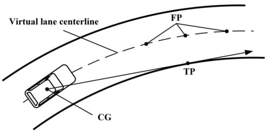
Figure 1.
Two visual strategies in curve driving.
To explain the disagreement, studies [34] have found that diverse scenarios and varying road designs can yield distinct outcomes, favoring one strategy over the other, that is gaze targets are influenced by the openness of the curve. What is more, drivers never look at a single location or object for a long time during driving, and the visual behavior is more like a scanning process with the rapid saccade–fixate–saccade pattern [35] for information selection and integration. There is nothing inherently incompatible between the TP and FP due to the flexibility of human visual behavior, and yet, the TP is the most-salient feature of the road edge in naturalistic driving conditions. Consequently, it may be more realistic to use different target points in different scenes when negotiating curves.
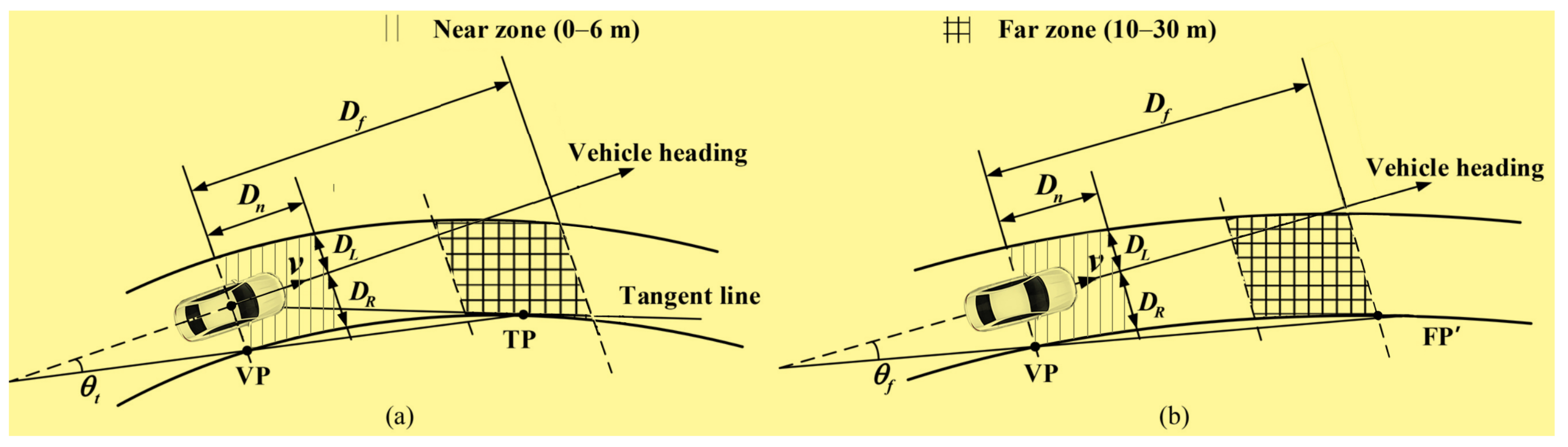
Based on the above analysis and understanding of the research findings on the visual perception mechanism and behavior in curve driving, the visual inputs (as illustrated in Figure 2) for steering control are determined with further explanations.

Figure 2.
Diagram for visual inputs of decision-making module: (a) when the TP is existent in the defined far zone; (b) when the TP is inexistent in the defined far zone.
- Vehicle longitudinal velocity v, which is a remarkable influence factor of human steering behavior except road curvature.
- Lateral deviation (), which reflects the vehicle’s lateral position in the lane at a near zone of the road ahead. It is derived from the relationship between the vehicle heading and the visible lane lines and does not need the information of the invisible centerline. denotes the distance between the vehicle heading and the left lane line 6 m ahead; denotes the distance between the vehicle heading and the right lane line 6 m ahead.
- Heading angle error ( when the TP is existent; when the TP is inexistent), which reflects the road curvature at a far zone of the future road, as well as the effect of the road geometry on the driver’s preview distance). denotes the angle between the vehicle heading and the line segment connecting the VP and TP; denotes the angle between the vehicle heading and the line segment connecting the VP and FP′.
The choice of the values of and needs to be specially explained here. The near point is defined as a close distance at which the driver can see the road through the front windshield; the specific far zone defined in our study was determined by referring to the relevant literature on the preview time [32,36], as well as according to the road curvature.
The process of screening, calculating, and obtaining the above perceivable visual inputs is termed the visual perception module in our driver model. It extracts the visual information that is available to the human driver and is the perception part of the driver model. More significantly, taking the vehicle motion feedback and the information of the near and far road ahead as the inputs for the steering decision, to some extent, can reflect human characteristics like the compensation control, preview behavior, and anticipation ability in the driving process.
The inputs of this module include vehicle motion states and road information. In the simulation, the outputs—speed, lateral deviation, and heading angle error—were obtained by the Lane Marker Sensor and some theoretical calculations in PreScan. The theoretical calculations included the vehicle dynamics model in MATLAB/Simulink, the computational formulas of the last two outputs (, ), and the tangent point information. In practical applications, these outputs of the visual perception module can also be obtained by the theoretical calculations and certain sensors.
2.2. Steering Control
With the perceived information of the surroundings and self-motion states, an appropriate steering action (steering wheel angle output) is selected from the knowledge base and experience of a driver in real-time for lateral control. The process of human driver’s perception and decisions is semantic and indistinct. In other words, there are much vagueness and randomness in the knowledge description and reasoning mechanism. The vehicle velocity, position, and heading, as well as road curvature are perceived in the form of natural language instead of accurate values. The decision-making for control behavior is based on experience and is difficult to explain clearly and describe precisely.
On account of these characteristics, ANFIS is a satisfactory way of modeling human drivers’ steering control. It is actually a fuzzy inference system implemented in the form of an ANN. On the one hand, it represents vague information using fuzzy sets and makes decisions in the form of if–then rules based on human knowledge and experience, which resembles the fuzzy inference behavior of humans. On the other hand, the rules can be acquired by learning from data, which resolves the complexity of the uncertainty and nonlinearity of the driver’s steering behavior.
Here, an ANFIS based on the Takagi–Sugeno model was adopted to map the relationship between the visual inputs and steering wheel angle. For a Sugeno-type fuzzy inference system with three inputs and one output, the if–then rules can be represented by the following general expression:
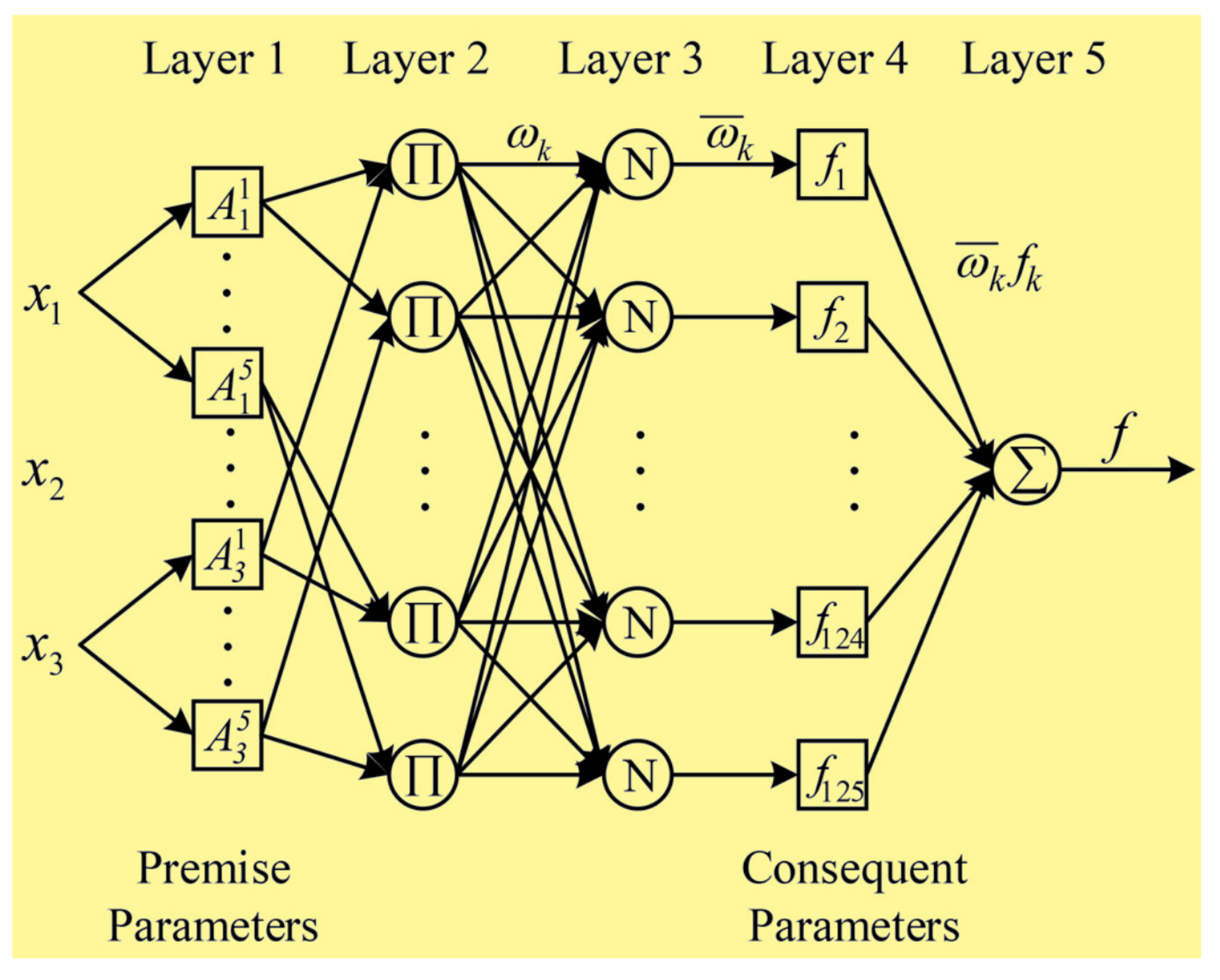
where are the input variables; is the linguistic label associated with the i-th input for the k-th rule; is the output of the k-th rule. Usually is the first-order polynomial of all input variables, ; when is a constant (called the zero-order T-S model), . The corresponding equivalent ANFIS architecture is formed by five feedforward layers, as shown in Figure 3. Each layer of ANFIS is explained below.
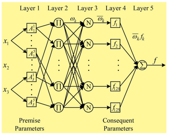
Figure 3.
Structure of ANFIS with 3 inputs, 1 output, and 125 rules.
Layer 1: In the first layer, also called the fuzzification layer, each input of the model is defined using five linguistic labels with triangular membership functions, as given in Equation (1):
where is the membership degree of the i-th input variable to the j-th fuzzy language; , , and are referred to as the “premise parameters”, which determine the shape of the membership function accordingly. Each adaptive node in this layer outputs a membership grade belonging to the corresponding set:
Layer 2: In the second layer, also called the rule layer, rules are generated, and each fixed node labeled with ∏ outputs the firing strength of the k-th rule by multiplying all input values calculated from the first layer:
Layer 3: In the third layer, also called the normalization layer, each fixed node labeled with N outputs a normalized value by calculating the ratio of the corresponding rule’s firing strength to the sum of all rules’ firing strengths:
Layer 4: In the fourth layer, also called the defuzzification layer, each adaptive node outputs a product of the normalized firing rule strength and rule value:
where the membership function type of each rule’s output is set to a constant value, and are referred to as the “consequent parameters”.
Layer 5: In the fifth layer, also called thew summation layer, there is a single and fixed node labeled with , and this calculates the final output of ANFIS by summing up all outputs from the fourth layer:
The ANFIS model was designed and trained by using the Neuro-Fuzzy Designer (ANFIS functions) in the MATLAB2016 software. After loading the data sets (which contain the training set and validation set, as stated in Section III Part E) and setting the number (five) and type (triangle) of the membership functions for each input variable and output variable, an initial Sugeno-type FIS structure was automatically generated using grid partitioning. The parameters of ANFIS were adjusted through the training process using a hybrid learning algorithm, which combines the least-squares and backpropagation gradient descent methods. The model was trained and updated until the set epochs was reached. The training epochs were set by trial and error with the aim of achieving the minimum training error.
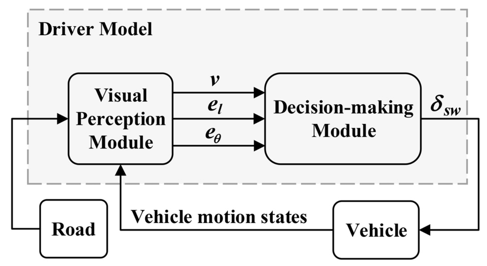
In combination with the above, a human-like driver model is proposed from visual perception to steering control. The overall structure of the driver model is shown in Figure 4. With regard to the visual perception module, it tries to extract the same perceivable information that human drivers actually use, such as the vehicle velocity, the vehicle lateral position in the lane through peripheral vision, and a preview of the upcoming road through the gaze behavior. With regard to the decision-making module, an ANFIS was adopted to mimic the fuzzy description and reasoning mechanism of humans and to construct the nonlinear mapping from the visual inputs to the steering wheel angle driven by the data.

Figure 4.
Structure of the driver model.
3. Collection of Human Driving Data
There are two ways to obtain human driving data: real vehicle tests and simulation tests based on a driving simulator. A driving simulator experiment is not as realistic as a field test. However, compared with the field test, a driving simulator experiment has the advantages convenience, high efficiency, low cost, and safety. Specifically, it is easier to control the variables and collect the data, more economical to acquire large-sample data, and safer for the participants. Therefore, the method of the driving simulation test was used for data collection in this study.
3.1. Setup
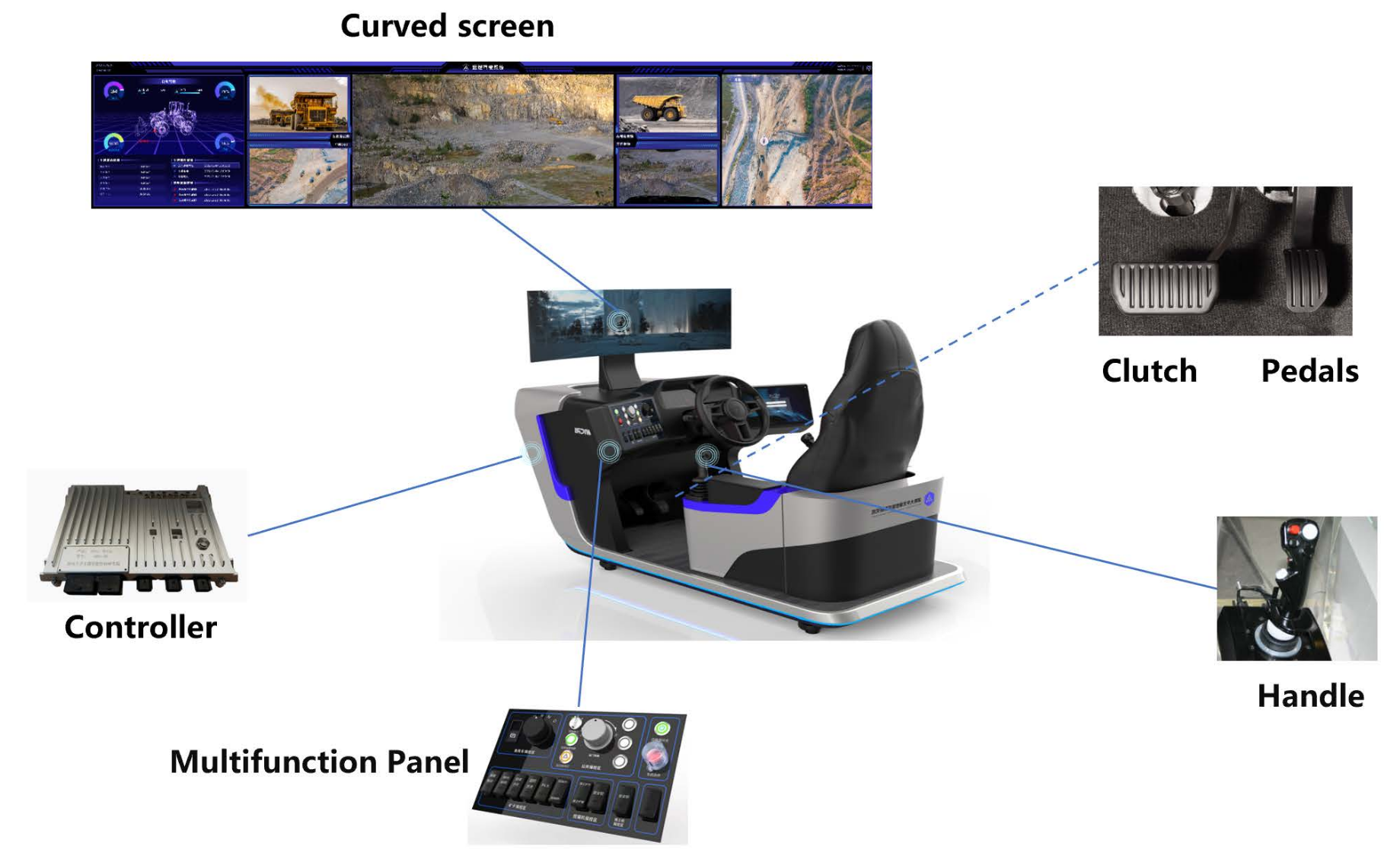
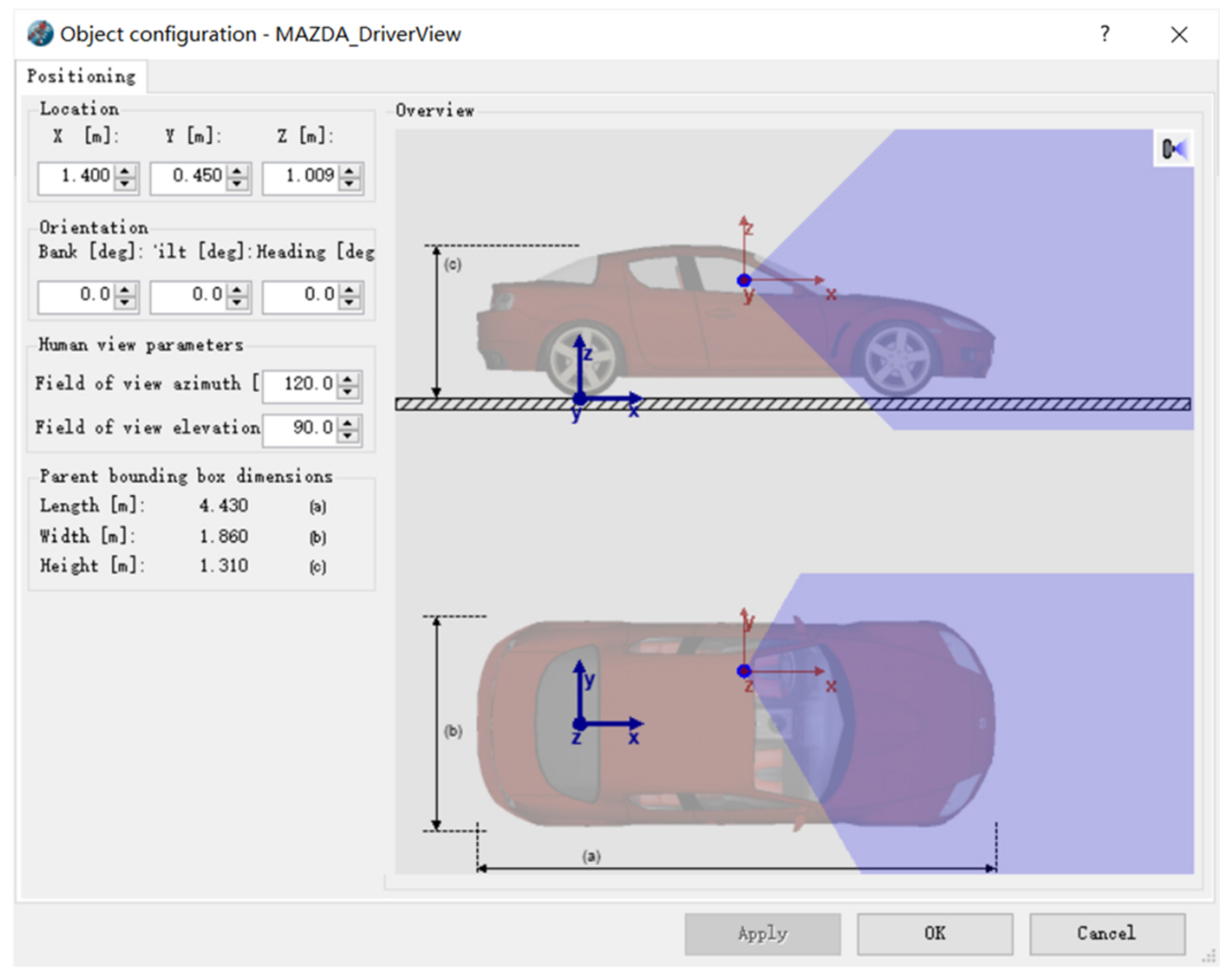
The driver-in-the-loop simulator was a virtual driving platform consisting of a 34-inch curved-display screen, a driving seat, and a set of Logitech G29 devices with a force feedback steering wheel, brake/acceleration pedals, clutch, and shift lever (as shown in Figure 5). It is acceptable and not unusual to use a similar driving simulation platform [37] for the study of driver behavior. The driving scenario was built based on PreScan. What is more, the range and angle of the view for the driver can be set up in “Human View” (as shown in Figure 6). The “2D Simple” vehicle dynamics model containing the driveline, engine, and steering was chosen in PreScan and generated in MATLAB/Simulink. It is capable of simulating a car’s longitudinal, lateral, and roll motion. The numerical values of some essential parameters of the vehicle model are listed in Table 2. The driver’s inputs acting on the Logitech G29 were transmitted to the virtual vehicle in PreScan, and then, the vehicle motion states and driver operation signals were collected and stored via the Simulink module with a sampling frequency of 100 Hz.
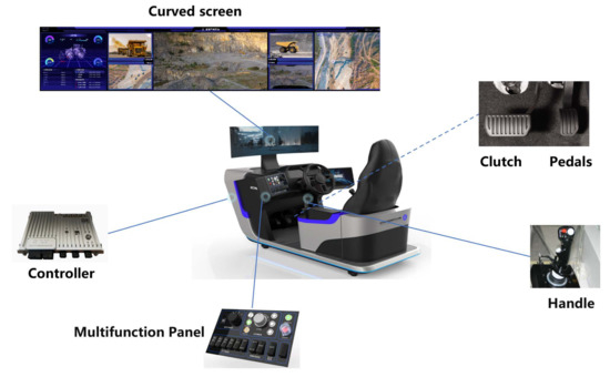
Figure 5.
Driver -in-the-loop simulation platform.

Figure 6.
“Human View” setting in PreScan. It is actually a camera for visual aid during simulation; we linked it to the vehicle and placed it at the position of the eyes of the driver, which can simulate the real driver’s view angle.
Table 2.
Parameters of the vehicle model.
3.2. Test Road
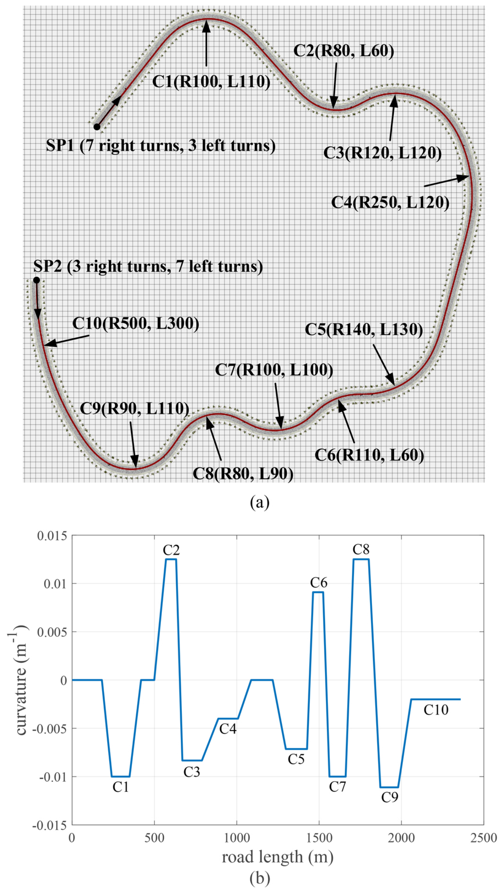
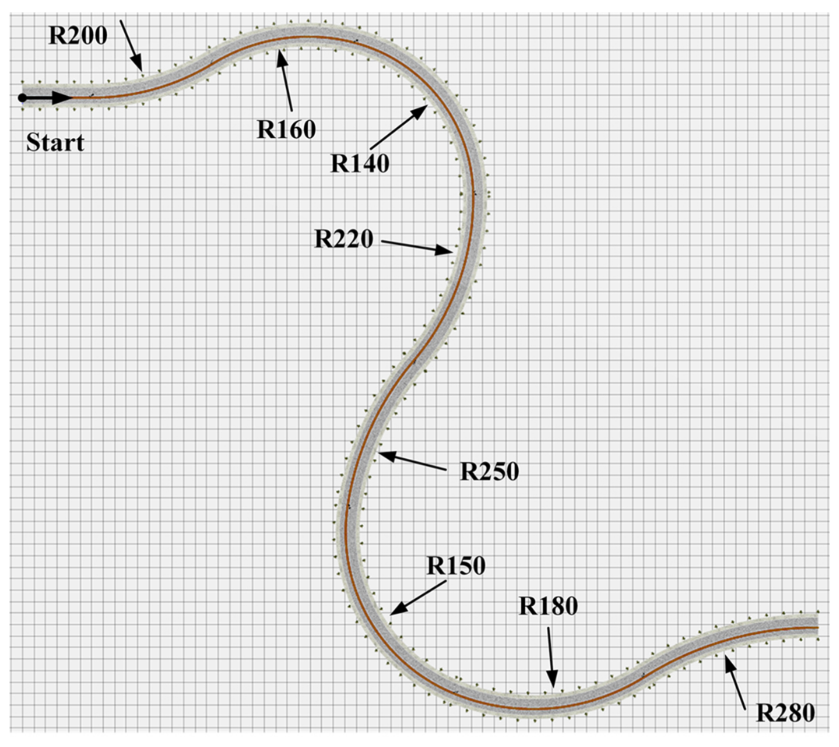
The experiments were conducted on a curved four-lane road in a horizontal plane. The width of each lane was 3.5 m. The test road was in total 2359.5 m in length, and road curvature changed continuously. It was built based on PreScan and linked by “straight road”, “spiral road”, and “bend road” segments (note that “straight road”, “spiral road”, and “bend road” are the terms of three types of road segments in the PreScan software). Among them, there were ten various circular curves with a radius from 80 m to 500 m. The details of each circular curve are shown in Figure 7. When taking SP1 as the start point, there were 7 right turns and 3 left turns; when starting from SP2, there were 3 right turns and 7 left turns.
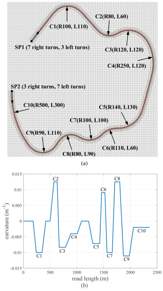
Figure 7.
Test road: (a) scenario in PreScan; (b) road curvature (SP1 is the start point).
3.3. Procedure
In consideration of the personalized driving style of different drivers, all driving data were collected by a human driver. The driver was a 26-year-old female with 4 years of driving experience. Research [13] has shown that, after repeated driving, the driving behavior of a human driver tends to stabilize, and even a novice driver can perform as well as an experienced driver. Therefore, to guarantee the training data were appropriate, the human driver was instructed to practice several times and adapt to the driving simulator experiment before the data collection. The driving route started from SP1 and SP2 separately. Longitudinal control of the vehicle was not considered in this study, and a PID controller was used to keep the vehicle at a specified longitudinal velocity, 20 km/h, 30 km/h, 40 km/h, 50 km/h, and 60 km/h, respectively. The human driver only needed to turn the steering wheel to control the vehicle’s direction by sensing the vehicle motion and road geometry from the visual display. Besides, to reduce accidental error and obtain more steering situations in curve driving as well, experiments of each speed on each driving route were conducted 20 times. Meanwhile, to some extent, the matter of the variability of human behavior was considered.
3.4. Tangent Point Information
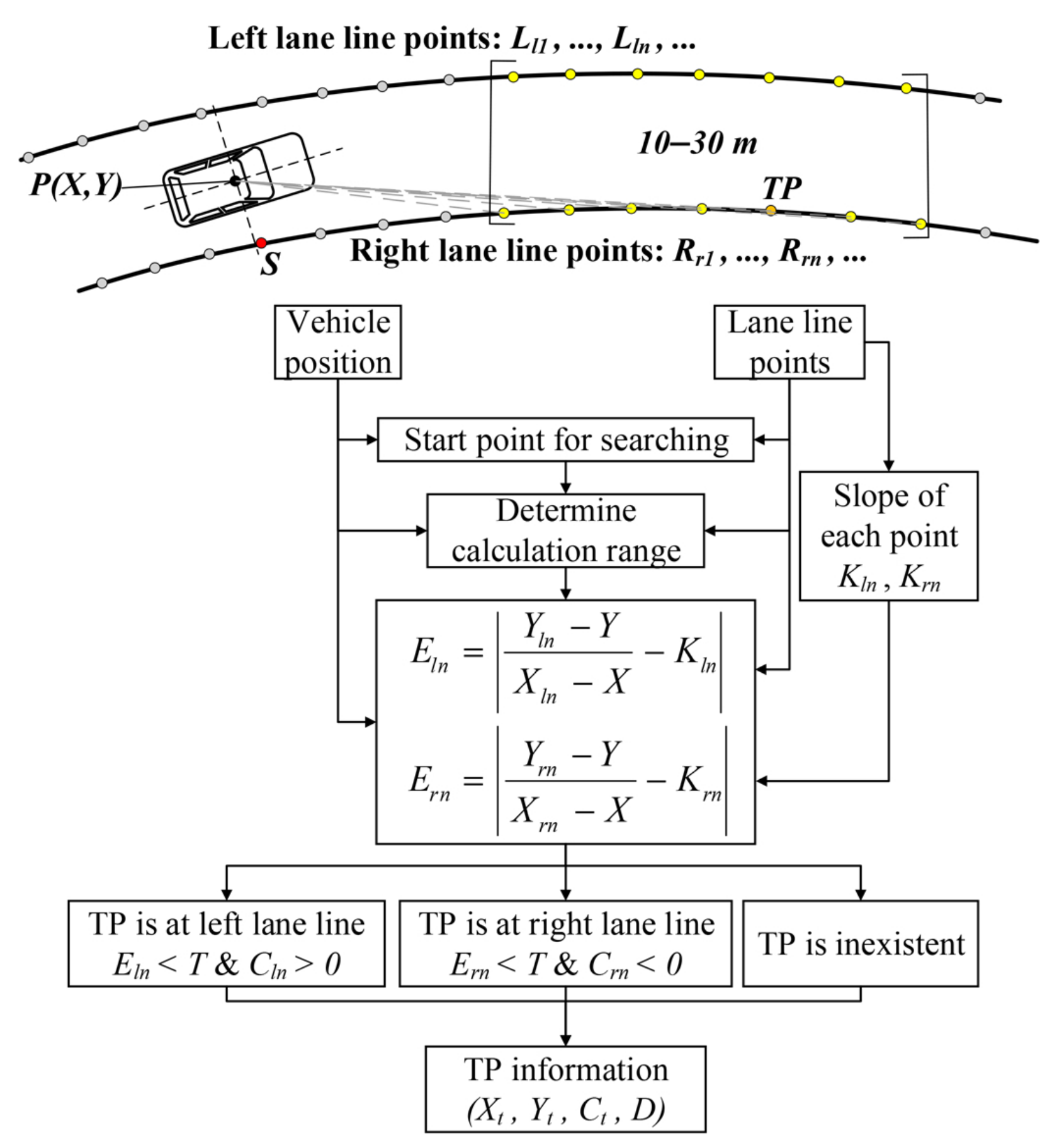
During the experiments, three kinds of data were collected: vehicle motion states (e.g., vehicle trajectory, velocity, yaw rate, acceleration, lateral deviation, and heading angle error), driver operation signals (steering wheel angle), and road information. These data were calculated and recorded by the vehicle dynamics model and the Lane Marker Sensor. The information of the tangent point needed to be further calculated and obtained according to the vehicle motion states and road information. Through the analysis, it was easy to know that the tangent point was not fixed in the dynamic visual scene when the vehicle was moving, and its position depended on both the road geometry and vehicle location. An approximate method for searching for the tangent point is described in Figure 8.

Figure 8.
An approximate method for searching for the TP.
Assume the starting point of the human driver’s sight line is at the CG of the vehicle; the position of the TP depends on the location of the vehicle on a curved road. The simulation results were composed of discrete data points. Similarly, the continuous road curves can be represented by sequential discrete points with position and curvature. Hence, the following:
- (1)
- The left and right lane lines were replaced with certain discrete points in an equidistant way: , ⋯, , ⋯; , ⋯, , ⋯. denotes the n-th point of the left lane line; denotes the n-th point of the right lane line; , , and denote the X-coordinate, Y-coordinate, and curvature of the n-th point on the left lane line; , , and denote the X-coordinate, Y-coordinate, and curvature of the n-th point on the right lane line.
- (2)
- Calculate the first-order difference quotient of two adjacent points, and use the value as an approximation for the slope of the tangent at certain positions on the certain lane line: ; . denotes the approximation for the slope of the tangent at the n-th point on the left lane line; denotes the approximation for the slope of the tangent at the n-th point on the right lane line; the value, to some degree, represents the heading at the corresponding position of the road.
- (3)
- Determine the start point (S) for searching, which is the point of the lane line nearest to the vehicle’s current position .
- (4)
- Determine the calculation range. Search the points of the lane lines from 10 to 30 m in front of the vehicle’s current position: ; .
- (5)
- Calculate the mathematical formulas: ; . denotes the slope of the segment connecting the CG of the vehicle and the n-th point on the left lane line; denotes the slope of the segment connecting the CG of vehicle and the n-th point on the right lane line.
- (6)
- Calculate the following mathematical formulas: ; . The calculated value shows the absolute difference between and ; shows the absolute difference between and .
- (7)
- If (a threshold value) and , the TP is the point satisfying ; if and , the TP is the point satisfying ; the coordinates of the TP , the curvature at the TP , as well as the distance between the TP and the vehicle can be obtained; if not, specify , , , and .
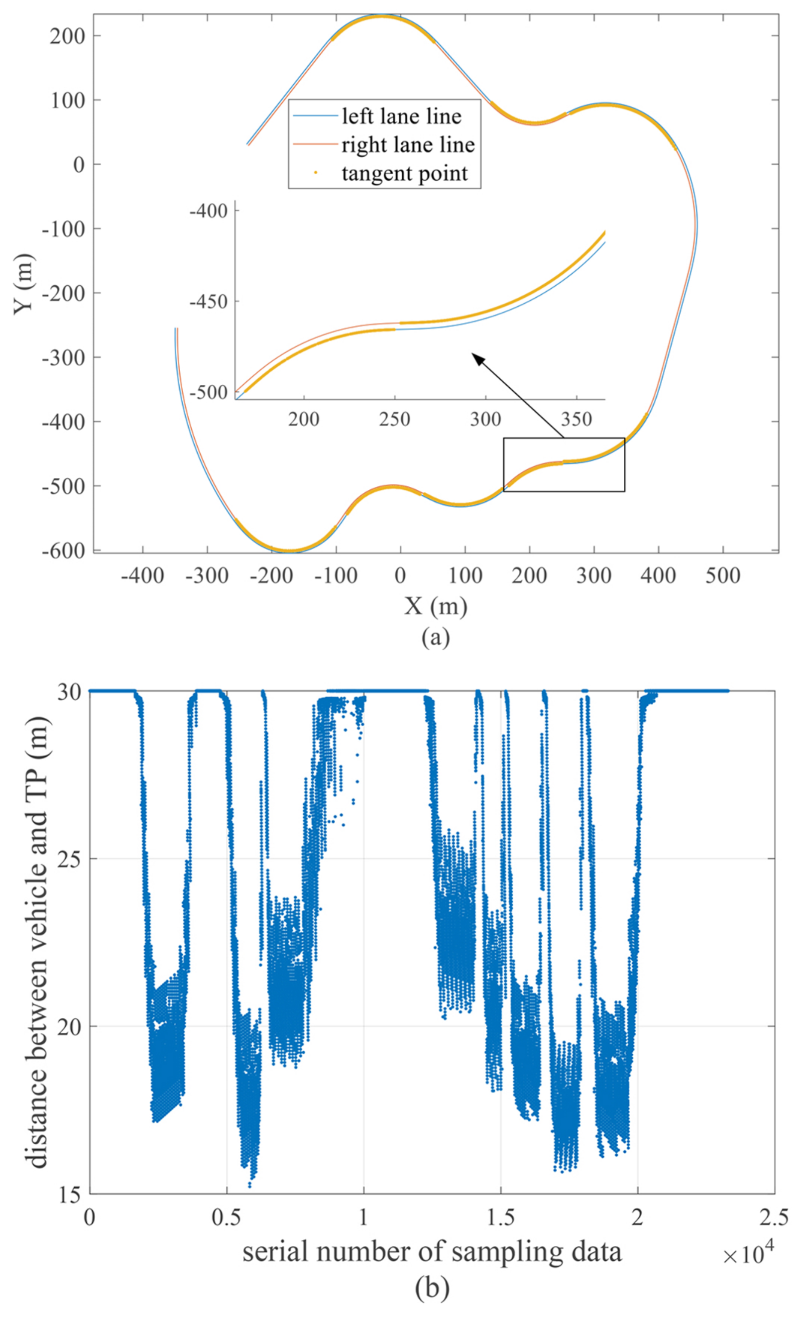
The TP information of one driving process is shown in Figure 9. As can be seen from Figure 9a, the tangent points (limited within 30 m ahead of the vehicle) were mainly located on the curved road with a big curvature. This also provides an intuitive understanding about which parts of the curved road the TP or FP information are respectively used as the inputs for the steering decision. In addition, analyzing the road curvature of Figure 7b, Figure 9b shows the value with the change of road curvature. We can clearly observe that the distance from the vehicle and TP decreases with the increase of the road curvature. Accordingly, the result suggests that the parameters related to the tangent point may reflect and present some road information in the driving process.

Figure 9.
TP information of one driving process: (a) TP distribution; (b) distance between the TP and vehicle. The distance between the vehicle and TP is denoted by ; the serial number of the sampling data can reflect the road length to some degree. It is noted that we define as 30 m when the TP is located outside the far zone. That is to say, is different from the actual distance between the vehicle and TP when the TP is inexistent within the range of 30 m.
3.5. Data Processing
From here, 200 (20 × 5 × 2) experiments were conducted, and 200 sets of driving data were collected. The data set used for ANFIS training was made up of three input variables and one output variable. The input variables were the vehicle longitudinal speed, lateral deviation at the near zone, and heading angle error at the far zone, which were acquired by the visual perception module, as mentioned earlier; the output variable was the steering wheel angle. In total, nearly 5.076 million pairs of input–output data were produced. All data were divided into two parts by a ratio of 8:2. Specifically, among the data of each speed and driving route, 16 sets were randomly selected as the training data, and the remaining 4 sets were taken as the validation data. Because the sampling interval was short and the vehicle speed was not too fast, the distance traveled by the vehicle to the adjacent data points was close; the driving data of the adjacent region also had little difference. Considering both the computing load and the diversity of driving situations, the data under 20 km/h, 30 km/h, 40 km/h, 50 km/h, and 60 km/h were filtered every 60, 40, 30, 24, and 20 data pairs, respectively. Finally, 116,817 pairs of data were used as the training set to train the ANFIS model, and 29,208 pairs of data were used as the validation set during the training to avoid overfitting.
Driven by the data, the ANFIS-based decision-making module for the steering wheel angle was obtained. Combined with the visual perception module for the visual inputs’ calculation, the human-like driver model proposed in Section II was ultimately established.
4. Model Simulation and Result Analysis
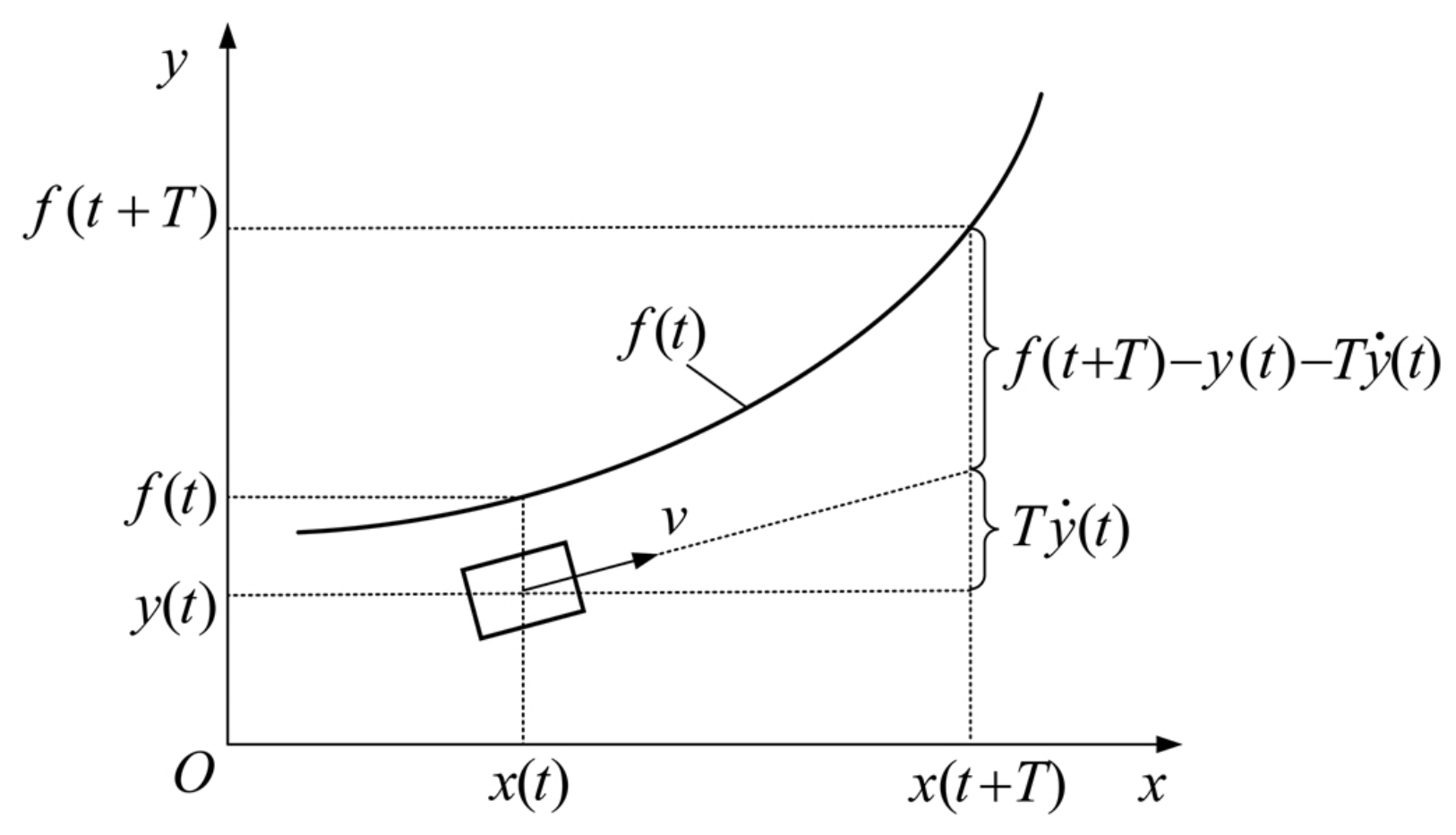
In order to validate the effectiveness and adaptability of the proposed human-like driver model, the model served as the lateral control algorithm of the vehicle and was demonstrated in the PreScan/MATLAB joint simulation environment. Furthermore, to make a comparative analysis with an existing driver model, the simulation of a common driver model—the single-point preview optimal curvature model—was added. As illustrated in Figure 10, the corresponding steering wheel angle was derived as:
where is the steering ratio, L is the wheel base, D is the preview distance, T is the preview time and set to 1 s in the simulation, and is the preview lateral deviation.

Figure 10.
Single-point preview optimal curvature model.
4.1. Validation Scenario and Speed
4.1.1. Validation on the Original Test Road
In view of the goal that the model is proposed to more truly represent human steering behavior, the model simulation results needed to be compared with the driving data of the human driver in the driving simulator. Twenty sets of the human driver’s steering data were separately collected at each of the six speeds—10 km/h, 20 km/h, 30 km/h, 40 km/h, 50 km/h, and 60 km/h—in Section III. To verify the effectiveness of the proposed model, the simulations of two models (the proposed human-like driver model and single-point preview optimal curvature model) were conducted on the same test road (as shown in Figure 5) with the corresponding speeds.
4.1.2. Validation on a New Test Road
Different vehicle motion states and road geometries have different visual inputs of the established human-like model and, then, influence the steering output generated by the model. Thus, it is meaningful to verify the adaptability of the model to various driving situations from the above two factors. First of all, a new multi-curvature curved road was built in PreScan. The road consisted of one straight segment for the start and eight curves with various radii, as shown in Figure 11. Based on this, the simulations of the two models and the driving simulator experiments were, respectively, carried out at speeds of 36 km/h and 54 km/h. Ten sets of the human driver’s steering data at each speed were collected. It needs to be made explicit that we chose a speed different from the training speeds to verify the applicability of the model to other driving speeds; of course, this can be replaced by any other value ranging from 10 km/h to 60 km/h, except for 10 km/h, 20 km/h, 30 km/h, 40 km/h, 50 km/h, and 60 km/h.
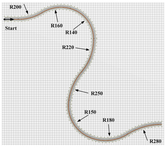
Figure 11.
New test road for validation.
4.2. Model Evaluation
Above all, to compare the different sets of driving data, all the time series data of the human driver and models needed to be converted into the data related to the road length. Then, the mean values of the human driving data of each test road and speed were taken for the following comparison and analysis.
For the quantitative analysis, the Pearson correlation coefficient (PCC), root-mean-squared error (RMSE), and mean absolute error (MAE) were used as the indexes to evaluate the model performance of human-like steering behavior. The PCC measures the similarity of the variation trends between two sets of data, with the following computational Equation (8). The RMSE and MAE measure the deviation of the numerical values between two sets of data, with the following computational Equations (9) and (10).
where H is the steering wheel angle of the human driver, M is the steering wheel angle of the model, and m is the total number of data points of the steering wheel angle. The closer the PCC value is to 1 and the smaller the RMSE and MAE values are, the more similar the two sets of data are.
4.3. Result and Analysis
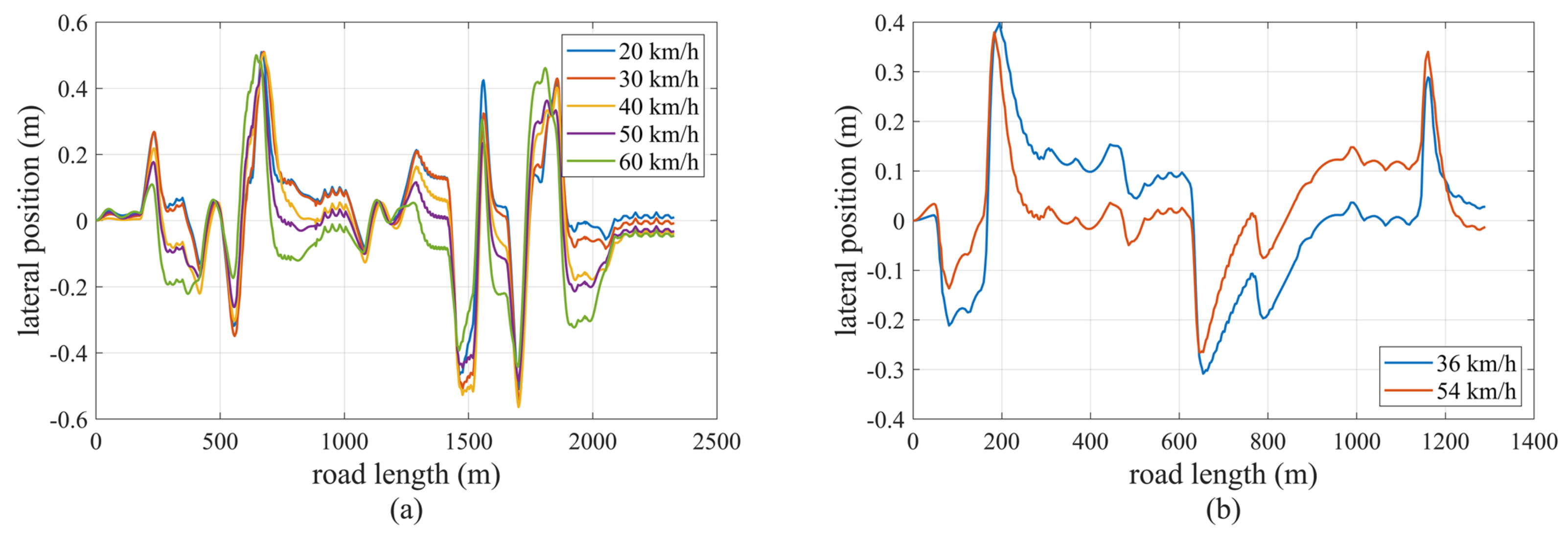
The simulation results of the vehicle’s lateral position of the proposed driver model on the two test roads are shown in Figure 12. The lateral position of the vehicle is defined as the distance (lateral deviation) between the vehicle’s current trajectory point and the virtual lane centerline; the value is positive if the vehicle is on the right side and negative if the vehicle is on the left side. On both test roads, all the lateral positions of the vehicle under different speeds varied in a certain range of to m, indicating that the vehicle was controlled to drive within the lane all of the time. Further, there was no risk of collision with vehicles on other lanes, and the driving safety can be guaranteed when the model is applied to vehicle lateral control. Thus, the simulation results demonstrated that the proposed human-like driver model had the basic ability of following and negotiating curved roads.

Figure 12.
Simulation results of lateral position of the proposed driver model: (a) on the original test road; (b) on the new test road.
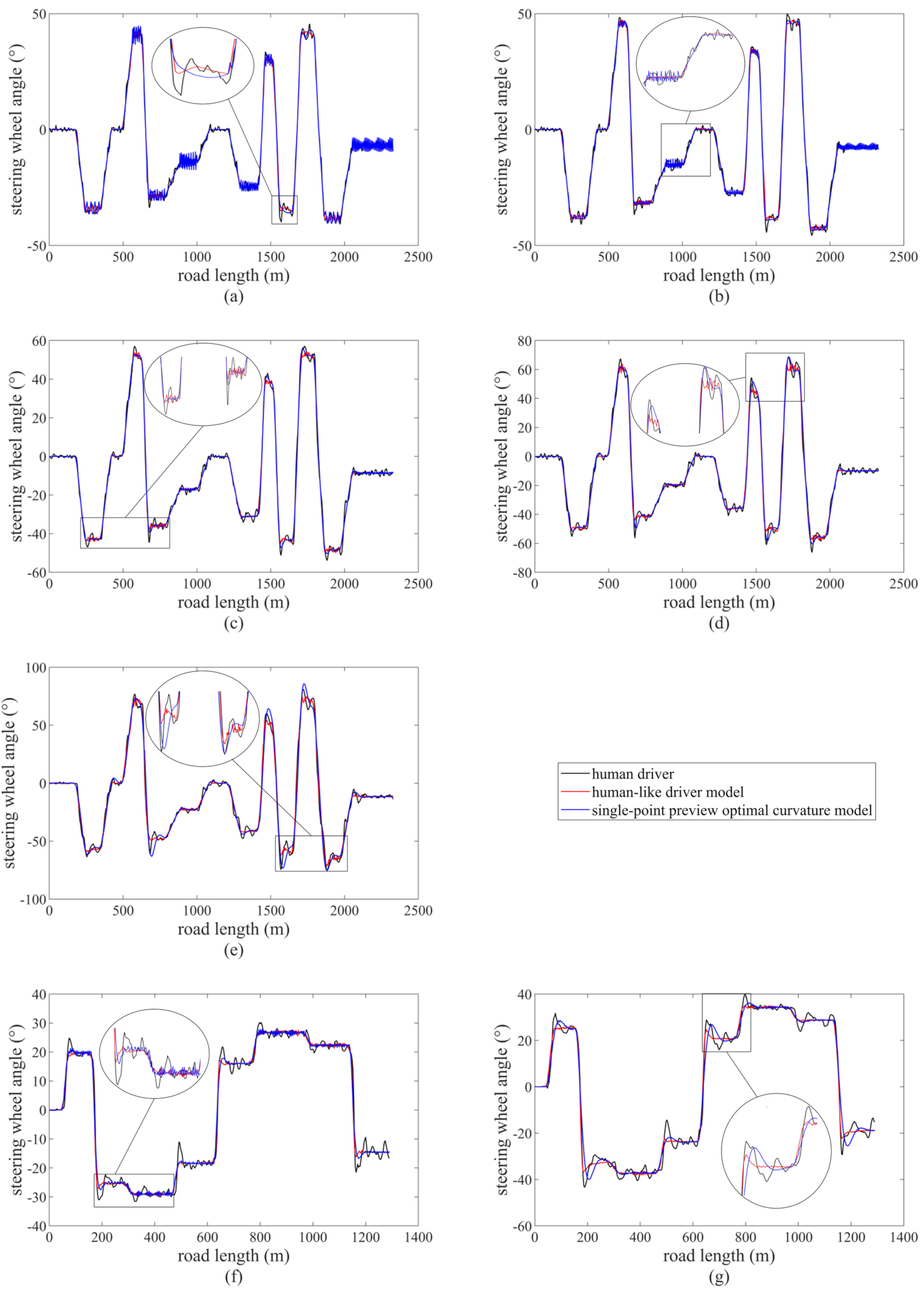
The steering wheel angles of the human driver and the two models were put together for comparison, as shown in Figure 13. Among them, (a)–(e) show the comparison of the steering wheel angles under the six speeds on the original test road and (f) and (g) show the comparison of the steering wheel angles under the other two speeds on the new test road. Overall, the steering wheel angles of the two models had a consistent variation tendency with the human driving data. The steering wheel angle values of the three basically coincided, as would be expected as well. Indeed, the shape of the steering wheel angle corresponded to that of the road curvature; because of the understeering characteristics, the amplitude of the steering wheel angle increases with the vehicle speed.
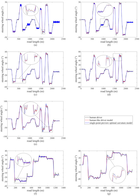
Figure 13.
Comparison of steering wheel angles: (a) on the original test road, at 20 km/h; (b) on the original test road, at 30 km/h; (c) on the original test road, at 40 km/h; (d) on the original test road, at 50 km/h; (e) on the original test road, at 60 km/h; (f) on the new test road, at 36 km/h; (g) on the new test road, at 54 km/h.
More specifically, it is clearly seen from Figure 13 that, for the human driver, there existed a few minor adjustments throughout the whole process of curve negotiation, rather than a single perfect steering maneuver, especially the overshooting of the steering wheel angle when entering each curve. As for the single-point preview optimal curvature model, the steering wheel angle jittered frequently and obviously when the vehicle negotiated some curves at a relatively low driving speed; the steering wheel angle showed overshooting when the vehicle entered each curve at a relatively high driving speed. By contrast, we observed that the steering wheel angle of the human-like driver model changed smoothly overall with some small fluctuations. Moreover, although the steering wheel angle of the proposed model sometimes changed more frequently than that of the human driver, it had a narrower fluctuation margin than that of the human driver.
It should be noted that not all steering behaviors exhibited by the human driver were good and worth mimicking. The steering wheel angle generated by the human-like driver model was smoother without overshooting compared to the human driver’s. We believe this shows the superiority of the proposed model. The probable reasons we analyzed were as follows. From the viewpoint of the human driving data, the overshooting of the steering wheel angle mainly occurred when entering each curve. Hence, this part of the driving data only accounted for a very small proportion of all the data and had little impact on the training of the ANFIS model, which was used as the decision-making module for the steering. From the viewpoint of the inputs of the steering decision, the visual perception module of the human-like driver model actually generalized this special situation. Besides, these inputs are defined as linguistic variables by fuzzification in ANFIS. Therefore, in the case of a small difference in the input values, the output—the steering wheel angle—may have little or no change.
Only from the visual comparison, the curve difference of the three steering wheel angles was not obvious. This needed further quantitative analysis. The calculation results of the performance indexes of the two models on the two test roads with the corresponding speeds are shown in Table 3. At 30 km/h to 40 km/h, some performance indexes showed that the steering wheel angle of the single-point preview optimal curvature model was closer to the human driver. However, overall, the PCC values of the human-like driver model were greater than that of the single-point preview optimal curvature model, and the RMSE and MAE values of the human-like driver model were smaller than that of the single-point preview optimal curvature model. The above results showed that, compared with the single-point preview optimal curvature model, the proposed human-like driver model had a higher correlation and a lower deviation compared to the steering wheel angle of the human driver.
Table 3.
Results of the performance indexes.
We can also find that the RMSE and MAE values increased with the driving speed. This is reasonable and acceptable for the further analysis. As we know, for the human driver, the steering control of the vehicle at a high speed generally is more difficult and has more variations than that at a low speed. Therefore, from the human driving data themselves, the difference between the different sets of driving data at a high speed was greater than that at a low speed; the difference between the human driving data and the model data was even greater.
In conclusion, there was a high similarity between the proposed human-like driver model and the human driver with respect to the steering wheel angle, indicating that the proposed model can represent certain human steering behaviors.
5. Conclusions
To conclude, a data-driven path-tracking model mimicking human drivers’ perception and decision-making was proposed in this paper. The visual perception module was established to extract visual inputs, which resembled the information perceived by human drivers. Considering the fuzzy characteristic and complexity of human behavior, an ANFIS driven by driving data was adopted to make the steering decision. Human driving data were collected via a driver-in-the-loop simulation platform. Learning from the data set, which contained the vehicle speed, lateral deviation at the near zone, and heading angle error at the far zone as the input variables and the steering wheel angle as the output variable, the ANFIS model was obtained. Finally, the driver model was demonstrated in the PreScan/MATLAB joint simulation environment.
With the proposed human-like driver model, vehicles are able to pass various curves successfully. Compared with the existing driver model, its steering behavior was more similar to the human drivers’. It was based on both theory and data, not entirely an “end-to-end” model. In other words, the inputs for the steering decision were extracted from the vehicle motion states and road scene. Therefore, it is adaptable to different driving conditions. In addition, because of the trained ANFIS model, the established driver model demonstrated a personalized driving style. The engineering application of the proposed method and the integrated longitudinal and lateral driver model will be our future research work.
Author Contributions
Conceptualization, Z.H. and Y.Y.; methodology, Z.H.; software, Z.Y.; validation, L.L.; formal analysis, H.Z.; investigation, Y.Z.; writing—original draft preparation, Z.H.; writing—review and editing, Y.Y.; visualization, L.L. All authors have read and agreed to the published version of the manuscript.
Funding
This research was funded by Zeyu Yang’s NSFC grant number 52202493 and Manjiang Hu’s NSFC grant number 52172384.
Data Availability Statement
Data are contained within the article.
Conflicts of Interest
Author Yue Yu was employed by the Bosch HUAYU Steering Systems Company. The remaining authors declare that the research was conducted in the absence of any commercial or financial relationships that could be construed as a potential conflict of interest.
References
- Chen, B.; Sun, D.; Zhou, J.; Wong, W.; Ding, Z. A future intelligent traffic system with mixed autonomous vehicles and human-driven vehicles. Inf. Sci. 2020, 529, 59–72. [Google Scholar] [CrossRef]
- Meng, L.Z.Q.; Chen, H. Kalman Filter-Based Fusion Estimation Method of Steering Feedback Torque for Steer-by-Wire Systems. Automot. Innov. 2021, 4, 430–439. [Google Scholar]
- Li, L.; Kaoru, O.; Dong, M. Human-like driving: Empirical decision-making system for autonomous vehicles. IEEE Trans. Veh. Technol. 2018, 67, 6814–6823. [Google Scholar] [CrossRef]
- McRuer, D.T.; Krendel, E.S. The human operator as a servo system element. J. Frankl. Inst. 1959, 267, 381–403. [Google Scholar] [CrossRef]
- Kondo, M.; Ajimine, A. Driver’s sight point and dynamics of the driver-vehicle-system related to it. In SAE Technical Paper; SAE International: Warrendale, PA, USA, 1968. [Google Scholar]
- MacAdam, C.C. Application of an optimal preview control for simulation of closed-loop automobile driving. IEEE Trans. Syst. Man, Cybern. 1981, 11, 393–399. [Google Scholar] [CrossRef]
- Zhou, X.; Jiang, H.; Li, A.; Ma, S. A new single point preview-based human-like driver model on urban curved roads. IEEE Access 2020, 8, 107452–107464. [Google Scholar] [CrossRef]
- Li, B.; Ouyang, Y.; Li, X. Mixed-Integer and Conditional Trajectory Planning for an Autonomous Mining Truck in Loading/Dumping Scenarios: A Global Optimization Approach. IEEE Trans. Intell. Veh. 2023, 8, 1512–1522. [Google Scholar] [CrossRef]
- Tan, Y.; Shen, H.; Huang, M.; Mao, J. Driver directional control using two-point preview and fuzzy decision. J. Appl. Math. Mech. 2016, 80, 459–465. [Google Scholar] [CrossRef]
- Li, Y.; Nan, Y.; He, J.; Feng, Q.; Zhang, Y.; Fan, J. Study on lateral assisted control for commercial vehicles. In Proceedings of the 2019 14th IEEE Conference on Industrial Electronics and Applications (ICIEA), Xi’an, China, 19–21 June 2019; pp. 567–572. [Google Scholar]
- Li, B.; Zhang, Y.; Zhang, T. Embodied Footprints: A Safety-Guaranteed Collision-Avoidance Model for Numerical Optimization-Based Trajectory Planning. arXiv 2023, arXiv:2302.076222023. [Google Scholar] [CrossRef]
- Land, M.; Horwood, J. Which parts of the road guide steering? Nature 1995, 377, 339–340. [Google Scholar] [CrossRef]
- Li, A.; Jiang, H.; Li, Z.; Zhou, J.; Zhou, X. Human-like trajectory planning on curved road: Learning from human drivers. IEEE Trans. Intell. Transp. Syst. 2020, 21, 3388–3397. [Google Scholar] [CrossRef]
- Macadam, C.C. Understanding and modeling the human driver. Veh. Syst. Dyn. 2003, 40, 101–134. [Google Scholar] [CrossRef]
- Marino, R.; Scalzi, S.; Netto, M. Nested pid steering control for lane keeping in autonomous vehicles. Control. Eng. Pract. 2011, 19, 1459–1467. [Google Scholar] [CrossRef]
- Piao, C.; Liu, X.; Lu, C. Lateral control using parameter self-tuning lqr on autonomous vehicle. In Proceedings of the 2019 International Conference on Intelligent Computing, Automation and Systems (ICICAS), Chongqing, China, 6–8 December 2019; pp. 913–917. [Google Scholar]
- Jiang, H.; Tian, H.; Hua, Y. Model predictive driver model considering the steering characteristics of the skilled drivers. Adv. Mech. Eng. 2019, 11, 1687814019829337. [Google Scholar] [CrossRef]
- Ling, R.; Shen, H.; Gu, J.; Mao, J.; Zhang, Y.; Miao, X.; Zhang, H. Vision based steering controller for intelligent vehicles via fuzzy logic. In Proceedings of the 2011 International Conference on Electronics and Optoelectronics, Dalian, China, 29–31 July 2011; Volume 4, pp. 417–420. [Google Scholar]
- Li, A.; Jiang, H.; Zhou, J.; Zhou, X. Implementation of human-like driver model based on recurrent neural networks. IEEE Access 2019, 7, 98094–98106. [Google Scholar] [CrossRef]
- Sentouh, C.; Chevrel, P.; Mars, F.; Claveau, F. A sensorimotor driver model for steering control. In Proceedings of the 2009 IEEE International Conference on Systems, Man and Cybernetics, San Antonio, TX, USA, 11–14 October 2009; pp. 2462–2467. [Google Scholar]
- Nash, C.J.; Cole, D.J. Modelling the influence of sensory dynamics on linear and nonlinear driver steering control. Veh. Syst. Dyn. 2018, 56, 689–718. [Google Scholar] [CrossRef]
- Nash, C.J.; Cole, D.J.; Bigler, R.S. A review of human sensory dynamics for application to models of driver steering and speed control. Biol. Cybern. 2016, 110, 91–116. [Google Scholar] [CrossRef] [PubMed]
- El, K.v.; Pool, D.M.; Mulder, M. Measuring and modeling driver steering behavior: From compensatory tracking to curve driving. Transp. Res. Part Traffic Psychol. Behav. 2019, 61, 337–346. [Google Scholar]
- Nash, C.; Cole, D. Identification and validation of a driver steering control model incorporating human sensory dynamics. Veh. Syst. Dyn. 2020, 58, 495–517. [Google Scholar] [CrossRef]
- Abduljabbar, R.; Dia, H.; Liyanage, S.; Bagloee, S.A. Applications of artificial intelligence in transport: An overview. Sustainability 2019, 11, 189. [Google Scholar] [CrossRef]
- Jang, J.R. Anfis: Adaptive-network-based fuzzy inference system. IEEE Trans. Syst. Man Cybern. 1993, 23, 665–685. [Google Scholar] [CrossRef]
- Salvucci, D.D. Modeling driver behavior in a cognitive architecture. Hum. Factors 2006, 48, 362–380. [Google Scholar] [CrossRef]
- Wang, W.; Mao, Y.; Jin, J.; Wang, X.; Guo, H.; Ren, X.; Ikeuchi, K. Driver’s various information process and multi-ruled decision-making mechanism: A fundamental of intelligent driving shaping model. Int. J. Comput. Intell. Syst. 2011, 4, 297–305. [Google Scholar]
- Schwarting, W.; Alonso-Mora, J.; Rus, D. Planning and decision-making for autonomous vehicles. Annu. Rev. Control. Robot. Auton. Syst. 2018, 1, 187–210. [Google Scholar] [CrossRef]
- Plöchl, M.; Edelmann, J. Driver models in automobile dynamics application. Veh. Syst. Dyn. 2007, 45, 699–741. [Google Scholar] [CrossRef]
- Wolfe, B.; Dobres, J.; Rosenholtz, R.; Reimer, B. More than the useful field: Considering peripheral vision in driving. Appl. Ergon. 2017, 65, 316–325. [Google Scholar] [CrossRef] [PubMed]
- Xing, D.; Li, X.; Zheng, X.; Ren, Y.; Ishiwatari, Y. Study on driver’s preview time based on field tests. In Proceedings of the 2017 4th International Conference on Transportation Information and Safety (ICTIS), Banff, AL, Canada, 8–10 August 2017; pp. 575–580. [Google Scholar]
- Lappi, O. Future path and tangent point models in the visual control of locomotion in curve driving. J. Vis. 2017, 14, 21. [Google Scholar] [CrossRef]
- Kandil, F.I.; Rotter, A.; Lappe, M. Car drivers attend to different gaze targets when negotiating closed vs. open bends. J. Vis. 2010, 10, 24. [Google Scholar] [CrossRef] [PubMed]
- Lappi, O.; Rinkkala, P.; Pekkanen, J. Systematic observation of an expert driver’s gaze strategy—An on-road case study. Front. Psychol. 2017, 8, 620. [Google Scholar] [CrossRef] [PubMed]
- Erwin, R. What preview elements do drivers need? IFAC Pap. Online 2016, 49, 102–107. [Google Scholar]
- Schnelle, S.; Wang, J.; Su, H.; Jagacinski, R. A personalizable driver steering model capable of predicting driver behaviors in vehicle collision avoidance maneuvers. IEEE Trans. Hum. Mach. Syst. 2017, 47, 625–635. [Google Scholar] [CrossRef]

Disclaimer/Publisher’s Note: The statements, opinions and data contained in all publications are solely those of the individual author(s) and contributor(s) and not of MDPI and/or the editor(s). MDPI and/or the editor(s) disclaim responsibility for any injury to people or property resulting from any ideas, methods, instructions or products referred to in the content. |
© 2023 by the authors. Licensee MDPI, Basel, Switzerland. This article is an open access article distributed under the terms and conditions of the Creative Commons Attribution (CC BY) license (https://creativecommons.org/licenses/by/4.0/).