Article

EEG_DMNet: A Deep Multi-Scale Convolutional Neural Network for Electroencephalography-Based Driver Drowsiness Detection

Computer of Science Department, College of Computer and Information Sciences, King Saud University (KSU), Riyadh 11432, Saudi Arabia
*
Author to whom correspondence should be addressed.
Electronics 2024, 13(11), 2084; https://doi.org/10.3390/electronics13112084
Submission received: 22 April 2024 / Revised: 19 May 2024 / Accepted: 22 May 2024 / Published: 27 May 2024
(This article belongs to the Special Issue Signal Processing and AI Applications for Vehicles)

Abstract

:
Drowsy driving is one of the major causes of traffic accidents, injuries, and deaths on roads worldwide. One of the best physiological signals that are useful in detecting a driver’s drowsiness is electroencephalography (EEG), a kind of brain signal that directly measures neurophysiological activities in the brain and is widely utilized for brain–computer interfaces (BCIs). However, designing a drowsiness detection method using EEG signals is still challenging because of their non-stationary nature. Deep learning, specifically convolutional neural networks (CNNs), has recently shown promising results in driver’s drowsiness. However, state-of-the-art CNN-based methods extract features sequentially and discard multi-scale spectral-temporal features, which are important in tackling the non-stationarity of EEG signals. This paper proposes a deep multi-scale convolutional neural network (EEG_DMNet) for driver’s drowsiness detection that learns spectral-temporal features. It consists of two main modules. First, the multi-scale spectral-temporal features are extracted from EEG trials using 1D temporal convolutions. Second, the spatial feature representation module calculates spatial patterns from the extracted multi-scale features using 1D spatial convolutions. The experimental results on the public domain benchmark SEED-VIG EEG dataset showed that it learns discriminative features, resulting in an average accuracy of 97.03%, outperforming the state-of-the-art methods that used the same dataset. The findings demonstrate that the proposed method effectively and efficiently detects drivers’ drowsiness based on EEG and can be helpful for safe driving.

1. Introduction

Drowsy driving is one of the leading causes of road accidents and deaths. A study conducted by the University Sleep Disorders Center at King Saud University revealed that drowsiness is one of the important causes of accidents in Saudi Arabia; the study showed that 33% of drivers were about to get involved in at least one accident because of drowsiness and 12% of drivers got in a real traffic accident because of sleeping while driving [1]. The American Automobile Association (AAA) reported that one-eighth (12.5%) of hospitalized passengers and drivers and one-sixth (16.5%) of deadly traffic accidents are caused by drowsy driving [2]. The German Road Safety Council estimates that 25% of highway traffic fatalities are caused by drowsy drivers [3]. These statistics show that drowsy driving is one of the leading causes of major traffic accidents.
Successful drowsiness detection is an important step in reducing the cost to society of traffic accidents, injuries, and death. Different measurements have been utilized to estimate drowsiness, including vehicle-based measurements, driver behavioral-based measurements, and physiological-based measurements. In view of physiological measurements, many existing studies have shown that EEG signals are the gold standard for drowsiness detection due to their direct relation to the brain where the drowsiness is initially triggered and due to their temporal information richness [4,5,6,7]. However, drowsiness detection using EGG signals is still hard due to the low signal-to-noise ratios and non-stationary nature of EEG signals [8,9,10]. Most of the existing studies that have been proposed to detect drivers’ drowsiness focus on features in each channel separately to detect drowsiness, making them vulnerable to variability across various subjects and sessions without sufficient data [11]. Therefore, the main goal of this study is to build a robust detection method for detecting drivers’ drowsiness, which can help alert drivers to safe driving.
The methods based on conventional machine learning techniques that use hand-engineered features for BCI tasks, including drowsiness detection, have been considered the standard for many years. However, deep learning-based methods have recently shown remarkable results in the BCI community [12]. Deep convolutional neural networks (CNNs) have the advantage of preserving the configurational and structural information in the original data and have been employed for drowsiness detection [10,13,14,15]. However, a CNN extracts features sequentially and disregards multi-scale spectral-temporal features, which can cause a serious problem in EEG signal features for different paradigms [13], subjects [16], and types [17]. Also, CNN-based methods require large amounts of training samples since they have a large number of trainable parameters [12], but BCI research generally contains a limited number of EEG experiments [16,18]. To mitigate these difficulties, we proposed an EEG_DMNet. The main contributions of this study are as follows:
  • We proposed a deep multi-scale CNN model (EEG_DMNet) based on EEG signals for driver’s drowsiness detection. This method takes an EEG trial as the input, preprocesses it using differential entropy (DE); then, it calculates multi-scale spectral-temporal features using 1D temporal convolution, and then computes the spatial patterns using 1D spatial convolutions.
  • We conducted several experiments to evaluate the performance of the method for drowsiness detection and compared its performance with those of the state-of-the-art methods, demonstrating its outstanding performance.
  • We gave an analysis and visualization of the features learned by the EEG_DMNet, which demonstrates that it learns more discriminative features compared to the state-of-the-art models.
The rest of this paper is organized as follows. Section 2 reviews previous studies in drowsiness detection using EEG brain signals with different methods, which can broadly be classified into two main categories, i.e., the methods based on hand-engineered features and those based on deep learning. Section 3 describes the proposed deep multi-scale CNN model (EEG_DMNet) for detecting drivers’ drowsiness. Section 4 describes the benchmark database used for experiments, the evaluation protocol, and the metrics used to validate the effectiveness of the proposed EEG_DMNet model and reports the experimental results. Section 5 discusses the results and findings. Finally, Section 6 concludes the paper.

2. Literature Review

Many researchers have addressed the problem of drowsiness detection using EEG brain signals, and different methods have been proposed. These methods can be broadly classified into two main categories, i.e., methods based on hand-engineered features and those based on deep learning. In the following sections, we throw light on some studies employing these methods.

2.1. Hand-Engineered (HE) Feature-Based Methods

The extracted features in the HE-based method for drowsiness detection fall into three main domains: time [19,20,21], frequency [11,22], and spatial domains. Moreover, multi-domain features have also been employed in HE-based methods. For instance, features that combine time and frequency domains [23] or time and spatial domains [24] have been used to improve classification accuracy.
For time domain features, Orru et al. [19] employed a one-dimensional Local Binary Pattern (1D-LBP) to extract features, while Khare and Bajaj et al. [21] extracted time domain statistical features selected by the Kruskal–Wallis test. Khare and Bajaj [20] also used the Kruskal–Wallis test to select time domain entropy-based features from the decomposed EEG signal using adaptive variational mode decomposition (AVMD).
Shen et al. [22] showed that drowsiness is detected using frequently used spectral spectrum features. However, EEG signals are aligned between each source subject and target subject to address cross-subject variations based on covariance minimization. In another method, Shen et al. [11] also used spectral spectrum features; however, decomposition transformed the data to a third-order tensor for feature extraction. To enhance the characteristic quality of the EEG signal, Min et al. [23] employed multi-entropy measures in both time and frequency domains. Chen et al. [24] extracted spatio-temporal features from EEG signals by computing the linear prediction cepstral coefficients (LPCCs) as the time domain features and the Riemann spatial covariance matrix as the spatial domain features.
As the features were extracted, different classifiers were utilized, such as SVM [11,19,24], random forest [25], logistic regression [23], etc.

2.2. Deep Learning (DL)-Based Methods

Different DL-based approaches have been used to extract deep features from EEG signals for drowsiness detection and classification, such as CNN [4,5,26,27,28,29], Recurrent Neural Networks (RNN), and Long Short-Term Memory (LSTM) [30,31], and other DL approaches [32].
Different CNN architectures have been used to extract features for drowsiness detection. Ko et al. [4] proposed a novel 1D CNN architecture that is independent of the input types or paradigms of EEG signals. It exploits spatial-spectral-temporal information from EEG signals at multiple scales with robust performance. In another method, Zue et al. [5] used the 1D CNNs with the Inception module and modified the AlexNet module to classify the EEG signals as awake or drowsy. Cui et al. [26] introduced a compact and interpretable 1D CNN model for discovering shared EEG features by combining the global average pooling (GAP) layer in the model structure and the Class Activation Map (CAM) method for localizing regions of the input signal to classify EEG signals. In another study, Cui et al. [27] introduced an interpretable 1D CNN to allow a sample-wise analysis of important features to classify EEG signals and take advantage of separable convolutions to process the EEG signals in a spatial-temporal sequence. In another study, Liqianga et al. [29] proposed a novel cross-dataset driver drowsiness recognition by introducing an entropy-guided robust feature (EGRF) adaptation framework that is based on an ICNN [26] as a baseline network to extract important features from the EEG signal. They proposed a deep unsupervised domain adaptation (UDA) technique to minimize the group-level drifts of EEG signal distribution.
Some researchers used LSTM, and others combined it with CNNs to extract features for drowsiness. Turkoglu et al. [30] converted the EEG signals into time frequency images using Short-Time Fourier Transform (STFT). Then, the rhythm images were extracted by dividing the EEG images based on frequency intervals. A pre-trained CNN model with pre-trained residual network ResNet models (i.e., ResNet18, ResNet50, and ResNet101) was used to extract features from each rhythm image and was then fed into the LSTM layer and finally classified. In another approach, Tang et al. [31] introduced a novel multi-channel LSTM network that efficiently learned the spatial correlation between multi-channel EEG signals. Also, to reduce individual variation between subjects, they proposed the Euclidean Space Data Alignment (ESDA) approach as a preprocessing step.
Some researchers used other DL approaches to extract features for drowsiness detection. Wang et al. [32] proposed a phase lag index graph attention network (PLI-GAT) that constructed a brain network to extract EEG time frequency features from multiple channels as a graph and then trained them using a GAT. It assigned weights to different neighbor nodes adaptively to enhance the expressiveness of the graph neural network model. In another method, Jai et al. [28] introduced an end-to-end temporal and graph convolution-based network (MATCN-GT). It consists of two kinds of blocks: a multi-scale attentional temporal convolutional neural network block (MATCN) to extract EEG features and a graph convolutional transformer block (GT) to process the extracted EEG features across different channels. They added a multi-scale attention module in the first block to ensure that channel correlation information is not lost. Also, they added a transformer module in the second block to perfectly capture the dependencies between long-distance channels.
Some studies incorporate both HE features and deep features. Budak et al. [30] proposed a hybrid method with three feature extraction techniques. Their proposed model was divided into three building blocks. In the first block, they extracted spectral entropy and instantaneous frequency features from the EEG spectrogram images and calculated energy distribution and zero-crossing distribution features from the raw EEG signals. In the second block, they used pre-trained AlexNet and VGGNet to extract deep features from EEG spectrogram images. In the third block, they used tunable Q-factor wavelet transform (TQWT) to decompose the EEG signals into sub-bands, and then they calculated the statistical features and spectrogram images of the sub-bands. An LSTM classifier was used in each block. Finally, the class label was predicted by taking a majority vote from all three blocks. Ko et al. [31] employed a method that uses a deep CNN and DE extracted from EEG signals. The network effectively extracts class-discriminative deep and hierarchical features, and finally, a densely connected layer is utilized for the final decision making to classify the driver’s state.
Based on the previous studies, there is a trend towards using deep learning methods instead of conventional methods, as they outperform HE methods. This can be explained by the nature of deep models that are less subjective to the initial assumptions about the features and their impressive classification performance at the expense of training dataset size and can achieve accuracy without overfitting. Though DL methods, namely, CNNs, have remarkable results in the BCI community and can detect meaningful patterns related to different mental states from complex EEG signals with acceptable accuracy, they extract features sequentially and disregard multi-scale spectral-temporal features, causing deficiency in EEG feature representation. Therefore, this issue needs further research.

3. Materials and Methods

In this section, we first formulate the problem and then present the details of the proposed EEG-based deep multi-scale CNN model (EEG_DMNet) for drivers’ drowsiness detection.

3.1. Problem Formulation

The problem is detecting the drowsiness of a subject (driver) using his/her EEG signal trial. It is a classification problem where the input EEG trial is used to predict the subject’s state. Let  x s   ϵ   R n C × n T  be a matrix representing an EEG trial of a subject s recorded using  n C  channels in  n T  timepoints and  y s ϵ Y = { a w a k e , t i r e d , d r o w s y } be the state of the subject s. Let  D s = x 1 s , y 1 s , x 2 s , y 2 s , x N s , y N s    be the annotated dataset collected from subject (s) where the goal is to design and learn a classifier  f : R n C × n T Y  that predicts the state  y ϵ Y  of an unknown EEG trial  x ϵ R n C × n T  as follows:
f x ; θ = y
where θ are the learnable parameters of  f .  Because of the outstanding performance of deep CNN models for various applications, we design  f  as a deep convolutional neural network, the EEG_DMNet, which learns multi-scale features from an EEG trial. The number of learnable parameters (weights and biases) of a deep CNN model is a challenging problem. To overcome this issue, the design of  f  is based on the pyramid architecture where the number of filters decreases as the depth increases [33], and it has a significantly smaller number of learnable parameters.

3.2. Proposed Deep Multi-Scale CNN Model—EEG_DMNet

The architecture of the proposed deep network in model  f  is depicted in Figure 1, and its complete specification is given in Table 1. It is an end-to-end function that takes an EEG trial x from a subject as the input, extracts discriminative features, and predicts its label, i.e., his/her state. It is composed of three mappings: (i) a spectral-temporal feature extractor ( F s t ), (ii) a spatial feature extractor ( F s ), and (iii) a classifier ( F c l ), i.e.,
y = f x ; θ = F c l F s F s t h x .
Here, h is the preprocessing procedure, which takes an EEG trial  x ϵ R n C × n T  as the input, preprocesses it is using differential entropy (DE) [34], which is calculated using Equation (2) [29] as follows:
h x = 1 2 π σ 2 e x μ 2 2 σ 2 l o g ( 1 2 π σ 2 e x μ 2 2 σ 2 ) d x .
The output of the preprocessing procedure  h x ϵ R n C × n T  is passed to the network for inference.
The mappings  F s t  and  F s  are parameterized with learnable parameters and learn discriminative features. The classifier  F c l  takes the learned features and predicts the label of the input EEG trial. The feature extractor mappings and the classifier are trained in an end-to-end manner. The details of each mapping are given in the following sections.

3.2.1. Spectral-Temporal Feature Extraction Mapping

This mapping extracts spectral-temporal features using four convolutions, one temporal convolution, and three temporal separable convolutions. It calculates multi-scale spectral information using three temporal separable convolutions. It takes the preprocessed EEG trial  h x  as the input and reshapes it in the dimensions of  n C n T 1 , i . e . ,   h x ϵ R n C × n T × 1 . The input is processed in a channel-wise manner, with the first temporal convolution consisting of  F 0  filters, which yields an activation  a T  of the dimension  n C n t F 0 , i.e.,  a T ϵ R n C × n T × F 0 . This activation is fed into three consecutive temporal separable convolutions in sequence. Formally, this function computes spectral-temporal features  H 1 1 , H 2 1 , H 3 1  at three scales, i.e.,
H 1 1 ,   H 2 1 ,   H 3 1 = F s t h x ; θ T , θ T S 1 , θ T S 2 , θ T S 3
where
H 1 1 = δ ψ T S 1 ψ T ( h x ;   θ T ,   θ T S 1 ) , H 2 1 = δ ψ T S 2 ( H 1 1 ;   θ T S 2 ) , H 3 1 = δ ψ T S 3 ( H 2 1 ;   θ T S 3 ) .
Here,  ψ T  is the temporal convolution,  ψ T S 1 ψ T S 2 , and  ψ T S 3  are three temporal separable convolutions with numbers of filters  F 1 F 2 , and  F 3 , and  δ  is leakyReLU non-linearity. Further,  θ T ,     θ T S 1 ,   θ T S 2 ,   a n d   θ T S 3  are the learnable parameters of  ψ T ψ T S 1 ψ T S 2 , and  ψ T S 3 , respectively. The outputs  H 1 1 ϵ R n C × n ˙ T × F 1 H 1 1 ϵ R n C × n ¨ T × F 2 , and  H 1 1 ϵ R n C × n T × F 3  are multi-scale spectral-temporal features, where  n ˙ T n ¨ T , and  n T  are temporal dimensions of the output features. The extracted features involve different frequency and temporal ranges, and the separable convolutions lead to a reduction in the number of model parameters. In all convolutions, we used the stride of one and zero padding.

3.2.2. Spatial Feature Extraction Mapping

The spatial feature extraction mapping calculates spatial patterns from the multi-scale spectral-temporal features  H 1 1 ,   H 2 1 ,   H 3 1  using three spatial convolutions. The output from each temporal separable convolution in  F s t  is fed in parallel to three spatial convolutions. Formally, it computes spatial patterns  G 1 1 ,   G 2 1 ,   G 3 1  from the multi-scale spectral-temporal features  H 1 1 ,   H 2 1 ,   H 3 1  as follows:
G 1 1 ,   G 2 1 ,   G 3 1 = F s H 1 1 ,   H 2 1 ,   H 3 1 ; θ S 1 , θ S 2 , θ S 3
where
G 1 1 = δ ϕ T S 1 ( H 1 1 ;   θ S 1 ) , G 2 1 = δ ϕ T S 2 ( H 2 1 ;   θ S 2 ) , G 3 1 = δ ϕ T S 3 ( H 3 1 ;   θ S 3 ) .
Here,  ϕ T S 1 ϕ T S 2  and  ϕ T S 3  are three spatial convolutions with the same number of numbers of filters, i.e.,  F 4  and a size of  n C × 1 ,  and  δ  is leaky ReLU non-linearity. Further,    θ S 1 ,   θ S 2 ,   a n d   θ S 3  are the learnable parameters of  ϕ T S 1 ϕ T S 2  and  ϕ T S 3 , respectively. The outputs  G 1 1 ϵ R 1 × n ˙ T × F 4 G 1 1 ϵ R 1 × n ¨ T × F 4 , and  G 1 1 ϵ R 1 × n T × F 4  are spatial patterns extracted from multi-scale spectral-temporal features. These are spatio-specral-temporal features that encode the compact brain activations in spatial, spectral, and temporal dimensions.

3.2.3. Classification Function

Finally, to predict the label of an EEG trial, the output from the spatial feature extraction mapping  F s  is fed to the classification function  F c l . It is composed of three mappings, i.e.,
y ^ = F c l G 1 1 ,   G 2 1 ,   G 3 1 ;   θ c l =   F φ χ G A P G 1 1 ,   G 2 1 ,   G 3 1 .
Here,  χ G A P :   R 1 × n ˙ T × F 4 R 1 × 1 × F 4  is the global average pooling that operates on each  G i 1 , i = 1,2 , 3  in parallel and pools the features along the temporal dimension, i.e.,
P i 1 = χ G A P ( G i 1 ) , i = 1,2 , 3
where  P i 1 R 1 × 1 × F 4 . It helps to reduce the feature dimension by reducing the redundancy in the feature space.
Next,  φ : R 1 × 1 × F 4 × R 1 × 1 × F 4 × R 1 × 1 × F 4 R 1 × 1 × 3 F 4  is the concatenation that concatenates the features obtained from  χ G A P  for each of  G i 1 , i = 1,2 , 3 , i.e.,
P = P 1 1 ,   P 2 1 ,   P 3 1 = φ P 1 1 ,   P 2 1 ,   P 3 1
Finally, the pooled and concatenated features  P R 1 × 1 × 3 F 4  are flattened and passed to the classifier  F , which is composed of an FC layer and a softmax activation and yields the posterior probability  p ( C i x )  of each class  C i ,   i = 1,2 , 3 , where
p i = p ( C i x ) = e a i j = 1 3 e a j ,   i = 1,2 , 3 .
Here,  a i ,   i = 1,2 , 3  are activations of the FC layer, which consists of three neurons because there are three classes  a w a k e , t i r e d , d r o w s y .  The most probable class is the predicted class of the input EEG trial  x .

4. Experiments and Results

In this section, we first describe the dataset used to evaluate the performance of the proposed method, and then we provide details of the experimental setup and the evaluation procedure. Finally, we give the results of the experiments, which were performed to validate the usefulness of the proposed method.

4.1. Dataset Description

To validate the effectiveness of the EEG_DMNet, we used the SEED-VIG EEG dataset [35,36], as it has been widely used for developing and testing the deep models for drowsiness detection of three classes, i.e., awake, tired, or drowsy. It is a public domain multimodal dataset published in 2017 by Zheng et al. [35] for vigilance estimation. This dataset contains EEG signals of 23 subjects, which were recorded for approximately 2 h at different times, i.e., night and noon, in a simulated driving environment. The subjects were 12 females and 11 males, with 23.3 years of average age and a 1.4 standard deviation. Each experiment has 885 trials, and each trial is 8 s in length. All participants had normal or corrected-to-normal vision; they were instructed to refrain from taking alcohol, caffeine, and tobacco before the experiment. The EEG signals were recorded using 17 channels (i.e., FT7, FT8, T7, T8, TP7, TP8, CP1, CP2, P1, PZ, P2, PO3, POZ, PO4, O1, OZ, and O2) according to the 10–20 system and sampled at 200 Hz. They are processed by applying a band-pass filter between 1 Hz and 75 Hz to filter out any noise and artifacts and are then segmented into eight-second non-overlapping trials. We used the raw EEG data of all twenty-three subjects from four channels (FT7, FT8, T7, and T8), as preferred for real-world applications [35]. The EEG data were labeled using three categories based on the PERCLOS labels [35], which denoted the percentage of eye closing time over total time. Therefore, we classified data into three classes, i.e., awake, tired, and drowsy, with two threshold values (0.35 and 0.7) [5,37]. The awake class was when PERCLOS < 0.35, the tired class was when 0.35 ≤ PERCLOS < 0.7, and the drowsy class was when PERCLOS ≥ 0.7.

4.2. Training and Evaluation Setup

In this section, we highlight the details of the training and evaluation of the EEG_DMNet.

4.2.1. Implementation and Training

We implemented the EEG_DMNet using the MATLAB Deep Learning Toolbox R2022b. We used commonly used cross-entropy loss and an Adam optimizer to learn the model with a learning rate of 0.001. We set the maximum number of epochs equal to 100, and the minimum batch size was set equal to 256. Additionally, all tunable parameters in this network are initialized by the He initializer, and all layers are activated by the leaky rectified linear unit (lReLU) function, except for the decision-making layer. We used training and validation datasets to train the model and an independent test dataset for testing.

4.2.2. Evaluation Protocol

To perform experiments and evaluate the performance of the proposed model, we used the subject-independent protocol, as it has been widely used, to divide the dataset into a training set (80%), validation set (10%), and testing set (10%) with the 10-fold cross-validation approach for evaluation. Using this protocol, the trials from all subjects are combined and randomly shuffled, and an equal number of trials from each class (4049 trials from each class) are selected. There are 9717 trials for training, 1215 trials for validation, and 1215 trials for testing. Then, the ten-fold cross-validation approach is used for evaluation, dividing the trials into ten folds. Each time, eight folds are used for training, one fold is used for validation, and one fold is used for testing. This process is repeated for each fold one by one. Therefore, all folds are used for training, validation, and testing, so the robustness of the model is tested over various samples.
To measure the performance of the proposed model, we used accuracy (Acc), sensitivity (Sen), specificity (Spe), precision (Pre), and F1 score. The effectiveness of the classification method depends on providing high rates on these metrics.

4.3. Ablation Study

The model involves a number of hyper-parameters, and the best choice of these hyper-parameters is essential for the best performance of the model. We performed several experiments with different hyper-parameter values to evaluate their effectiveness and choose the values that give the best performance.

4.3.1. Raw Data vs. DE Preprocessing

Firstly, we evaluated our proposed model using raw EEG data and DE preprocessing. The results are shown in Table 2, and it is clear from the results that using the DE preprocessing is better than using raw EEG data in terms of all metrics.

4.3.2. The Impact of the Number of Filters

We conducted many experiments with different numbers of filters. The results are shown in Table 3; it is clear from the results that  F 0 = F 1,4 = F 2,4 = F 3,4 = 1024  attain the best performance metrics. This means that a large number of multi-scale temporal and spatial patterns must be extracted using a large number of multi-scale filters.

4.3.3. The Impact of Activation Functions

The activation functions in the temporal and spatial convolution layers play a key role and impact the overall performance of the model. We examined three well-known activations, i.e., ReLU, LeakyReLU, and ELU, for our model. The results shown in Table 4 indicate that LeakyReLU performs better than the other two activations. The reason is probably that ReLU can result in neurons dying because they suffer from saturation when the input is negative. ELU, on the other hand, is computationally intensive.

4.3.4. The Impact of Spectral-Temporal and Spatial Blocks

The proposed model consists of two main blocks: spectral-temporal and spatial blocks. The spectral-temporal block learns spectral and temporal features, whereas the spatial block learns the spatial features. To show the effectiveness of each block, we performed experiments with and without spatial blocks. The results are shown in Table 5, which highlights the importance of spatial blocks. Only the spectral-temporal block is not enough to learn the discriminative features.

4.3.5. The Impact of Scales

The proposed model uses different scales to learn the hierarchy of features at different scales. The question is which number of scales is the best. To find the answer to this question, we conducted experiments with different numbers of scales. The results of three different choices are presented in Table 6. It is clear from the results that the three scales yield the best performance. The three scales help the model to learn discriminative features at different scales, which are important in discriminating different states of the subject.

4.3.6. The Impact of RNN Layers

In addition, we investigated whether long-range dependencies play a role in learning discriminative features. We performed many experiments by adding a sequence folding layer after the input layer and the LSTM/BiLSTM/GRU layer before the classification layer in the EEG_DMNet model. The experimental results showed that the BiLSTM layer is better than the LSTM and GRU layers. The results are shown in Table 7; it is shown from the results that the EEG_DMNet without the LSTM/BiLSTM/GRU layer has the best performance in terms of all metrics and has fewer learnable parameters. It indicates that long-range dependencies in an EEG trial do not have a significant role in discriminating the brain states as awake, tired, or drowsy.

4.4. Experiment Results

After determining the best hyper-parameter choices and selecting the best configuration of the EEG_DMNet model, we conducted experiments to examine the effect of the driving time on the performance of the proposed model; we performed experiments using the noon trials, night trials, and both trials with the EEG_DMNet model and 10-fold cross-validation. The results are shown in Table 8, Table 9 and Table 10; it is clear from the results that the noon trials had the best performance metrics in both trials and, finally, the night trials. This is because during the day, the three states, awake, tired, or drowsy, are more discriminative, i.e., a driver is either awake or feeling tired or drowsy. During the night time, the states are not as discriminative as during the day time, and there is a possibility that these states are very close to each other, causing difficulty for the system.

4.5. Comparison with the State-of-the-Art Methods

We compared the EEG_DMNet model with the state-of-the-art methods that used the same dataset. As shown in Table 11, the EEG_DMNet model outperforms the state-of-the-art methods, with the highest performance metrics in detecting drivers’ drowsiness based on EEG signals.
So far, the state-of-the-art method that gives the best performance on the SEED-VIG EEG dataset is the VIGNet model proposed by Ko et al. [38]. This method first computes the DE features from an EEG trial and then passes it to a deep CNN model (VIGNet). For comparison with this model, we implemented this model and tested it using DE features with 10-fold cross-validation. We obtained 89.72%, 84.58%, 92.29%, 84.67%, and 84.60% for accuracy, sensitivity, specificity, precision, and F1 score, respectively. Additionally, we implemented the MSNN by Ko et al. [4] and obtained 81.62%, 72.43%, 86.21%, 72.68%, and 72.11% for accuracy, sensitivity, specificity, precision, and F1 score, respectively. We could not obtain the same results as reported in the VIGNet and the MSNN; the difference might be due to the implementation tool and the split of data for training, validation, and testing. However, we implemented and tested it using the same environment, and the split of data that was used for the EEG_DMNet model for a fair comparison. We employed a Wilcoxon rank-sum test with alpha = 0.05 to statistically analyze the EEG_DMNet against the VIGNet and MSNN and check whether the EEG_DMNet is statistically superior to its comparator. Table 12 reports the p-values of the Wilcoxon test. It shows that the median of the EEG_DMNet is greater than the VIGNet and MSNN at a 5% significance level, which means that the EEG_DMNet is better than the VIGNet and MSNN, and the difference is significant at a 5% significance level since p-values are less than alpha and h = 1. Thus, we concluded that the EEG_DMNet is statistically superior to the VIGNet and MSNN.
Furthermore, we analyzed the complexity of the models and reported the results in Table 13. As shown in the table, the EEG_DMNet parameter complexity is higher than the VIGNet and the MSNN, which enhances its capacity to learn the discriminative features.
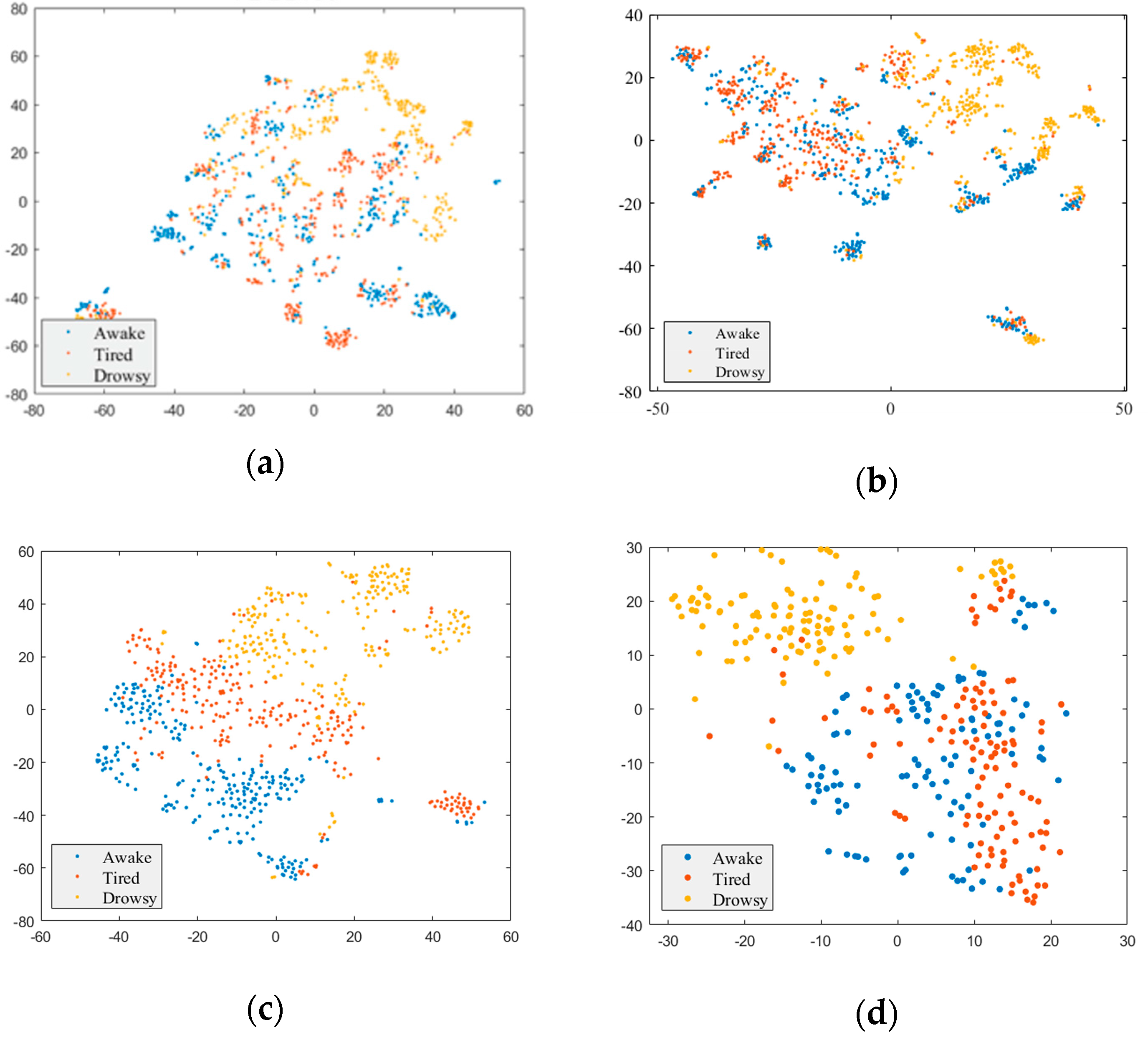
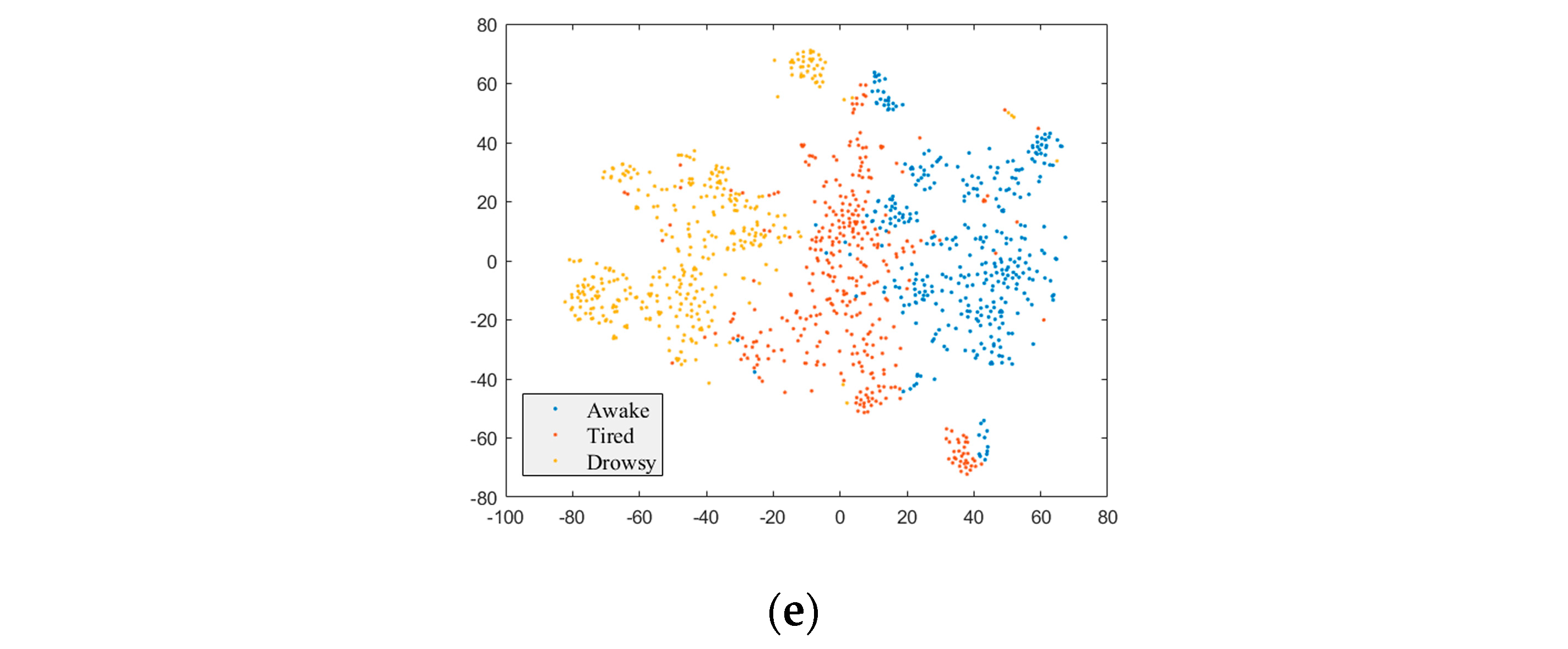
We analyzed the features extracted from the EEG_DMNet using t-Distributed Stochastic Neighbor Embedding (t-SNE). Figure 2 illustrates the extracted features after plotting using the t-SNE method for the VIGNet, the MSNN, and the EEG_DMNet. The blue points represent the awake class, the red points represent the tired class, and the yellow points represent the drowsy class. The figure shows that the VIGNet and the MSNN exhibit a poor representation of clustering features since the awake class, tired class, and drowsy class samples are mixed, and there is no clear boundary between them. In contrast, the EEG_DMNet shows a better clustering effect. Also, in the figure, we can see that the EEG_DMNet with the noon trials and both noon and night trials make a separate cluster for each class. While the EEG_DMNet with the night trials make a separate cluster for the drowsy class sample, the awake class and tired class samples are mixed, and there is no clear boundary between them. The confusion matrices that are achieved by the VIGNet, MSNN, and EEG_DMNet are illustrated in Figure 3, which is consistent with the distribution of the features plotted by t-SNE. In the figure, the EEG_DMNet is better than the VIGNet and MSNN using noon trials, night trials, and both noon and night trials.

5. Discussion

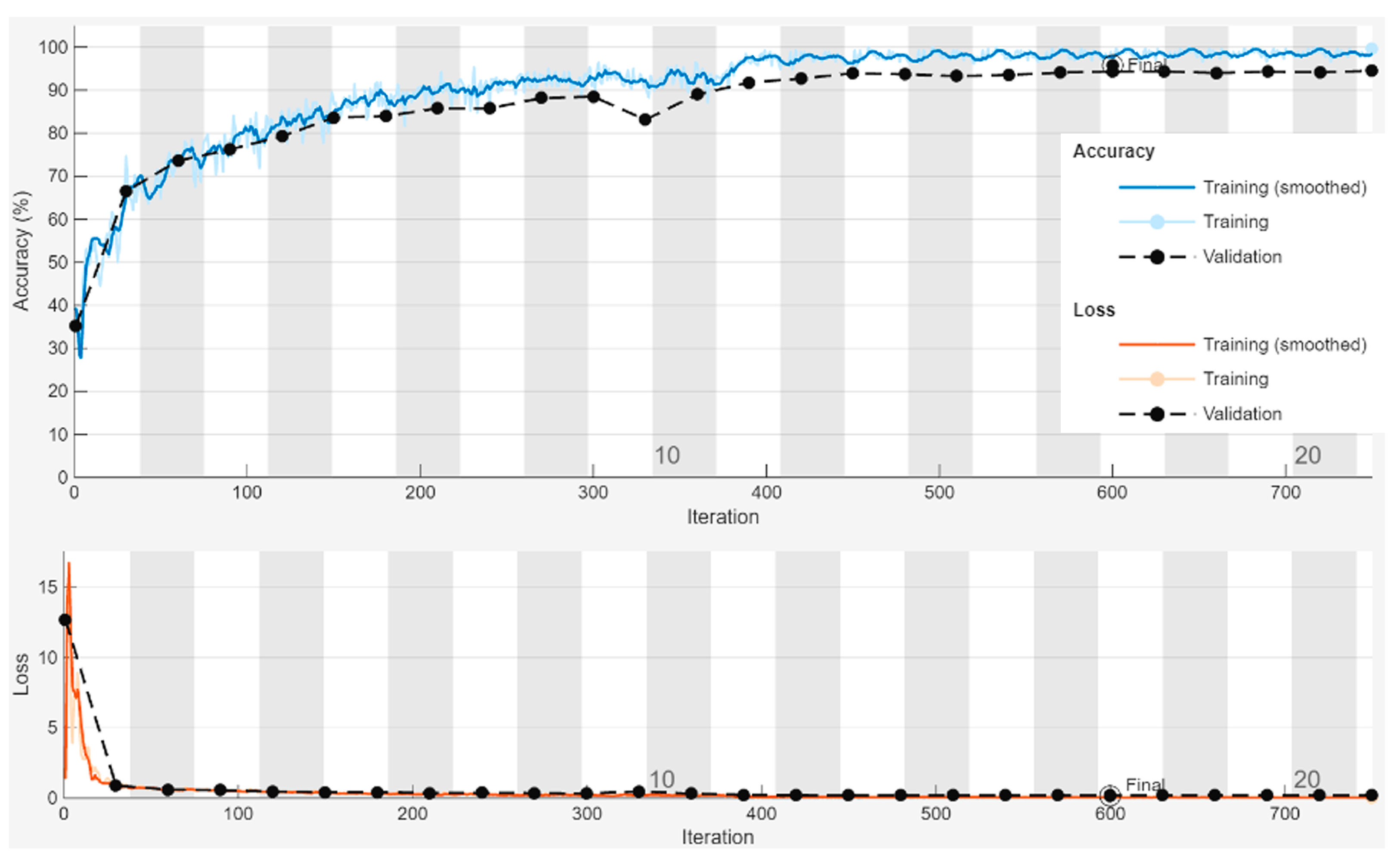
The experimental results showed that the EEG_DMNet learns discriminative features relevant to drowsiness perfectly, as shown by clusters of the features when analyzed with t-SNE. Also, it is statistically superior to the VIGNet and the MSNN when analyzed with the Wilcoxon rank sum test. Furthermore, its parameter complexity is higher than that of the VIGNet and MSNN, which enhances its capacity to learn discriminative features. The analysis of the training and validation curves during the training process reveals that there is no overfitting despite having a higher number of learnable parameters (shown in Figure 4). In addition to that, the EEG_DMNet outperforms state-of-the-art methods that use the same dataset and have the best performance metrics. It achieved performance with an average accuracy of 97.46% and an average F1 score of 96.09% for the noon trials, 96.90% and 95.33% for the night trials, and 97.03% and 95.53% for both trials. These findings demonstrate that preprocessing the EEG signal using DE and employing the pyramid architecture in the EEG_DMNet model contributed to achieving the best-proposed model with the best results in detecting drivers’ drowsiness based on EEG signals.

6. Conclusions

Drowsy driving is one of the main factors of millions of deaths and injuries around the world. An accurate detection method for drivers’ drowsiness helps in decreasing the side effects of this problem. An electroencephalogram (EEG) is one of the most common ways to detect a driver’s drowsiness. Recently, deep learning, especially CNNs, has outperformed traditional machine learning methods in many applications since it learns the appropriate features from the data in an automatic way. However, the CNN extracts features sequentially and disregards multi-scale spectral-temporal features, which can cause a serious problem in EEG signal features. This paper proposed a solution to the driver’s drowsiness detection problem by introducing a deep multi-scale CNN model (EEG_DMNET), which exploited spatial-spectral-temporal features from EEG signals at multiple scales for tackling the non-stationarity of EEG trials. The experimental results showed that the proposed method learns discriminative features, outperforming the state-of-the-art methods that used the same dataset and improving the generalization capability. This method will be useful for detecting drowsiness and alerting drivers to prevent traffic accidents caused by drowsiness accurately and in real time with immediate feedback. Moreover, such AI-based techniques can be improved over time with more data and easily integrated with other modalities, such as facial expressions and vehicle behavior. Even though EEG requires physical sensors, the rapid advancements in sensor technology, including wireless EEG headsets, enable AI to optimize data collection and processing while improving accuracy and sensitivity. However, these devices still require further enhancement to capture accurate signals, whereas the most commonly used EEG headsets are uncomfortable for continuous use in real driving and are vulnerable to environmental noise, such as vehicle/driver motion. Another challenge affecting such systems’ reliability is the variability of EEG signals between individuals, especially with the scarcity of EEG data, which necessitates ongoing research to address these issues and implement techniques that can benefit from transferring knowledge from subject to subject. Considering these issues, in our future work, we will evaluate the proposed model using the leave-one-subject evaluation protocol, analyze the individual variations, and find the learning techniques to overcome the issues due to individual variations.

Author Contributions

Conceptualization, H.B.O. and M.H.; methodology, M.H. and H.B.O.; software, H.B.O.; validation, H.B.O., M.H., and R.A.; formal analysis, H.B.O., R.A., and M.H.; investigation H.B.O. and M.H.; resources, H.B.O. and R.A.; data curation, H.B.O. and R.A.; writing—original draft preparation, H.B.O. and R.A.; writing—review and editing, M.H.; visualization, R.A.; supervision, M.H.; project administration, M.H.; funding acquisition, M.H. All authors have read and agreed to the published version of the manuscript.

Funding

The research was supported under the Researchers Supporting Project number (RSP2024R109), King Saud University, Riyadh, Saudi Arabia.

Data Availability Statement

We used a public domain dataset [35].

Conflicts of Interest

The authors declare no conflicts of interest.

References

  1. Studying the Prevalence of Drowsiness among Car Drivers in Saudi Arabia and Its Impact on Accidents. University Sleep Disorders Center at King Saud University. Available online: https://news.ksu.edu.sa/ar/node/104565 (accessed on 24 May 2022).
  2. Tefft, B. The Prevalence and Impact of Drowsy Driving—AAA Foundation for Traffic Safety. Available online: https://aaafoundation.org/prevalence-impact-drowsy-driving/ (accessed on 30 April 2022).
  3. Akerstedt, T.; Bassetti, C.; Cirignotta, F.; García-Borreguero, D.; Gonçalves, M.; Horne, J.; Léger, D.; Partinen, M.; Penzel, T.; Philip, P.; et al. Sleepiness at the Wheel; The French institut of Sleep and Vigilance: Paris, France, 2013. [Google Scholar]
  4. Ko, W.; Jeon, E.; Jeong, S.; Suk, H.I. Multi-scale Neural Network for EEG Representation Learning in BCI. IEEE Comput. Intell. Mag. 2021, 16, 31–45. [Google Scholar] [CrossRef]
  5. Zhu, M.; Chen, J.; Li, H.; Liang, F.; Han, L.; Zhang, Z. Vehicle driver drowsiness detection method using wearable EEG based on convolution neural network. Neural Comput. Appl. 2021, 33, 13965–13980. [Google Scholar] [CrossRef] [PubMed]
  6. Gharagozlou, F.; Saraji, G.N.; Mazloumi, A.; Nahvi, A.; Nasrabadi, A.M.; Foroushani, A.R.; Kheradmand, A.A.; Ashouri, M.; Samavati, M. Detecting Driver Mental Fatigue Based on EEG Alpha Power Changes during Simulated Driving. Iran. J. Public Health 2015, 44, 1693–1700. [Google Scholar] [PubMed]
  7. Lin, C.T.; Wu, R.C.; Liang, S.F.; Chao, W.H.; Chen, Y.J.; Jung, T.P. EEG-based drowsiness estimation for safety driving using independent component analysis. IEEE Trans. Circuits Syst. I Regul. Pap. 2005, 52, 2726–2738. [Google Scholar] [CrossRef]
  8. Paulo, J.R.; Pires, G.; Nunes, U.J. Cross-Subject Zero Calibration Driver’s Drowsiness Detection: Exploring Spatiotemporal Image Encoding of EEG Signals for Convolutional Neural Network Classification. IEEE Trans. Neural Syst. Rehabil. Eng. 2021, 29, 905–915. [Google Scholar] [CrossRef] [PubMed]
  9. Cuui, Y.; Xu, Y.; Wu, D. EEG-Based Driver Drowsiness Estimation Using Feature Weighted Episodic Training. arXiv 2019, arXiv:1909.11456. [Google Scholar] [CrossRef] [PubMed]
  10. Ko, W.; Yoon, J.; Kang, E.; Jun, E.; Choi, J.-S.; Suk, H.-I. Deep Recurrent Spatio-Temporal Neural Networkfor Motor Imagery based BCI. In Proceedings of the 6th International Conference on Brain-Computer Interface (BCI), Gangwon, Republic of Korea, 15–17 January 2018; AAAI Press: Washington, DC, USA, 2018; pp. 1–3. [Google Scholar]
  11. Shen, M.; Zou, B.; Li, X.; Zheng, Y.; Zhang, L. Tensor-Based EEG Network Formation and Feature Extraction for Cross-Session Driving Drowsiness Detection. In Proceedings of the 42nd Annual International Conference of the IEEE Engineering in Medicine & Biology Society (EMBC), Montreal, QC, Canada, 20–24 July 2020. [Google Scholar]
  12. Schirrmeister, R.T.; Springenberg, J.T.; Fiederer, L.D.J.; Glasstetter, M.; Eggensperger, K.; Tangermann, M.; Hutter, F.; Burgard, W.; Ball, T. Deep learning with convolutional neural networks for EEG decoding and visualization. Hum. Brain Mapp. 2017, 38, 5391–5420. [Google Scholar] [CrossRef]
  13. Lawhern, V.J.; Solon, A.J.; Waytowich, N.R.; Gordon, S.M.; Hung, C.P.; Lance, B.J. EEGNet: A Compact Convolutional Network for EEG-based Brain-Computer Interfaces. J. Neural Eng. 2016, 15, 056013. [Google Scholar] [CrossRef]
  14. Chen, J.; Wang, S.; He, E.; Wang, H.; Wang, L. Recognizing drowsiness in young men during real driving based on electroencephalography using an end-to-end deep learning approach. Biomed. Signal Process. Control 2021, 69, 102792. [Google Scholar] [CrossRef]
  15. Cui, J.; Lan, Z.; Sourina, O.; Müller-Wittig, W. EEG-Based Cross-Subject Driver Drowsiness Recognition with an Interpretable Convolutional Neural Network. IEEE Trans. Neural Netw. Learn. Syst. 2022, 34, 7921–7933. [Google Scholar] [CrossRef]
  16. Jayaram, V.; Alamgir, M.; Altun, Y.; Scholkopf, B.; Grosse-Wentrup, M. Transfer Learning in Brain-Computer Interfaces. IEEE Comput Intell Mag 2016, 11, 20–31. [Google Scholar] [CrossRef]
  17. Arico, P.; Borghini, G.; Di Flumeri, G.; Sciaraffa, N.; Babiloni, F. Passive BCI beyond the lab: Current trends and future directions. Physiol. Meas. 2018, 39, 08TR02. [Google Scholar] [CrossRef] [PubMed]
  18. Haufe, S.; Meinecke, F.; Görgen, K.; Dähne, S.; Haynes, J.-D.; Blankertz, B.; Bießmann, F. On the interpretation of weight vectors of linear models in multivariate neuroimaging. Neuroimage 2014, 87, 96–110. [Google Scholar] [CrossRef] [PubMed]
  19. Orrù, G.; Micheletto, M.; Terranova, F.; Marcialis, G.L. Electroencephalography Signal Processing Based on Textural Features for Monitoring the Driver’s State by a Brain-Computer Interface. arXiv 2020, arXiv:2010.06412. [Google Scholar]
  20. Khare, S.K.; Bajaj, V. Entropy-Based Drowsiness Detection Using Adaptive Variational Mode Decomposition. IEEE Sens. J. 2021, 21, 6421–6428. [Google Scholar] [CrossRef]
  21. Khare, S.K.; Bajaj, V. Optimized Tunable Q Wavelet Transform Based Drowsiness Detection from Electroencephalogram Signals. IRBM 2022, 43, 13–21. [Google Scholar] [CrossRef]
  22. Shen, M.; Zou, B.; Li, X.; Zheng, Y.; Li, L.; Zhang, L. Multi-source signal alignment and efficient multi-dimensional feature classification in the application of EEG-based subject-independent drowsiness detection. Biomed. Signal Process. Control 2021, 70, 103023. [Google Scholar] [CrossRef]
  23. Min, J.; Xiong, C.; Zhang, Y.; Cai, M. Driver fatigue detection based on prefrontal EEG using multi-entropy measures and hybrid model. Biomed. Signal Process. Control 2021, 69, 102857. [Google Scholar] [CrossRef]
  24. Chen, K.; Liu, Z.; Liu, Q.; Ai, Q.; Ma, L. EEG-based mental fatigue detection using linear prediction cepstral coefficients and Riemann spatial covariance matrix. J Neural Eng. 2022, 19, 066021. [Google Scholar] [CrossRef]
  25. Kim, K.J.; Lim, K.T.; Baek, J.W.; Shin, M. Low-Cost Real-Time Driver Drowsiness Detection based on Convergence of IR Images and EEG Signals. In Proceedings of the 3rd International Conference on Artificial Intelligence in Information and Communication, ICAIIC, Jeju Island, Republic of Korea, 13–16 April 2021; Institute of Electrical and Electronics Engineers Inc.: Piscataway, NJ, USA, 2021; pp. 438–443. [Google Scholar] [CrossRef]
  26. Jia, H.; Xiao, Z.; Ji, P. End-to-end fatigue driving EEG signal detection model based on improved temporal-graph convolution network. Comput. Biol. Med. 2023, 152, 106431. [Google Scholar] [CrossRef]
  27. Turkoglu, M.; Alcin, O.F.; Aslan, M.; Al-Zebari, A.; Sengur, A. Deep rhythm and long short term memory-based drowsiness detection. Biomed. Signal Process. Control 2021, 65, 102364. [Google Scholar] [CrossRef]
  28. Tang, J.; Li, X.; Yang, Y.; Zhang, W. Euclidean space data alignment approach for multi-channel LSTM network in EEG based fatigue driving detection. Electron. Lett. 2021, 57, 836–838. [Google Scholar] [CrossRef]
  29. Wang, Z.; Zhao, Y.; He, Y.; Zhang, J. Phase lag index-based graph attention networks for detecting driving fatigue. Rev. Sci. Instrum. 2021, 92, 094105. [Google Scholar] [CrossRef] [PubMed]
  30. Budak, U.; Bajaj, V.; Akbulut, Y.; Atila, O.; Sengur, A. An effective hybrid model for EEG-based drowsiness detection. IEEE Sens. J. 2019, 19, 7624–7631. [Google Scholar] [CrossRef]
  31. Ko, W.; Oh, K.; Jeon, E.; Suk, H.-I. VIGNet: A Deep Convolutional Neural Network for EEG-based Driver Vigilance Estimation. In Proceedings of the 2020 8th International Winter Conference on Brain-Computer Interface (BCI), Gangwon, Republic of Korea, 26–28 February 2020; IOP Publishing Ltd.: Bristol, UK, 2020; pp. 1–3. [Google Scholar] [CrossRef]
  32. Ullah, I.; Hussain, M.; Qazi, E.-U.; Aboalsamh, H. An automated system for epilepsy detection using EEG brain signals based on deep learning approach. Expert Syst. Appl. 2018, 107, 61–71. [Google Scholar] [CrossRef]
  33. Huo, X.-Q.; Zheng, W.-L.; Lu, B.-L. Driving Fatigue Detection with Fusion of EEG and Forehead EOG. In Proceedings of the 2016 International Joint Conference on Neural Networks (IJCNN), Vancouver, BC, Canada, 24–29 July 2016; pp. 897–904. [Google Scholar]
  34. Shi, L.-C.; Lu, B.-L. Off-Line and On-Line Vigilance Estimation Based on Linear Dynamical System and Manifold Learning. In Proceedings of the Annual International Conference of the IEEE Engineering in Medicine and Biology, Buenos Aires, Argentina, 31 August–4 September 2010; IEEE: Piscataway, NJ, USA, 2010; pp. 6587–6590. [Google Scholar]
  35. Cui, J.; Lan, Z.; Liu, Y.; Li, R.; Li, F.; Sourina, O.; Müller-Wittig, W. A compact and interpretable convolutional neural network for cross-subject driver drowsiness detection from single-channel EEG. Methods 2021, 202, 173–184. [Google Scholar] [CrossRef]
  36. Hwang, S.; Park, S.; Kim, D.; Lee, J.; Byun, H. Mitigating inter-subject brain signal variability for EEG-based driver fatigue state classification. In Proceedings of the ICASSP 2021—2021 IEEE International Conference on Acoustics, Speech and Signal Processing (ICASSP), Toronto, ON, Canada, 6–11 June 2021; Institute of Electrical and Electronics Engineers Inc.: Piscataway, NJ, USA, 2021; pp. 990–994. [Google Scholar] [CrossRef]
  37. Zheng, W.-L.; Lu, B.-L. A multimodal approach to estimating vigilance using EEG and forehead EOG. J. Neural Eng. 2017, 14, 026017. [Google Scholar] [CrossRef]
  38. Zhang, N.; Zheng, W.L.; Liu, W.; Lu, B.L. Continuous vigilance estimation using LSTM neural networks. In Lecture Notes in Computer Science (Including Subseries Lecture Notes in Artificial Intelligence and Lecture Notes in Bioinformatics); Springer: Berlin/Heidelberg, Germany, 2016; pp. 530–537. [Google Scholar] [CrossRef]
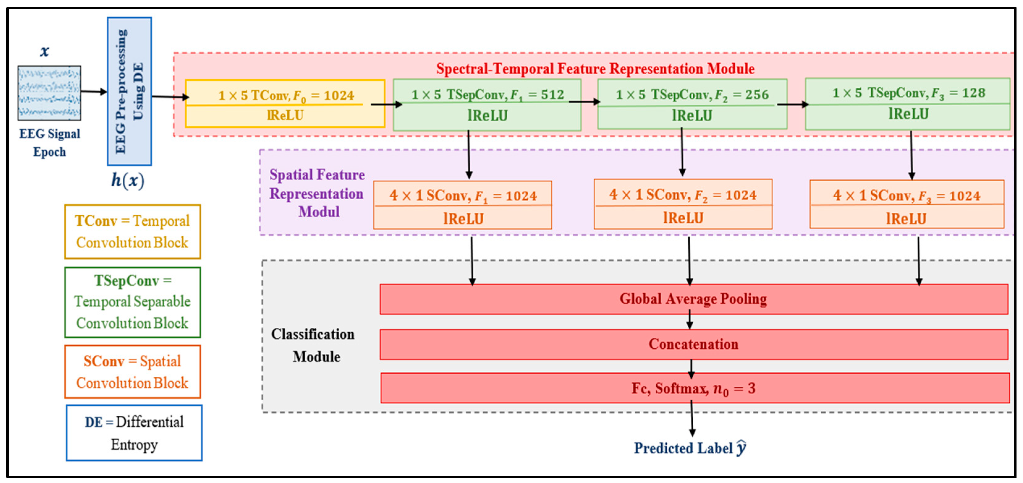
Figure 1. Detailed description of the architecture of the EEG_DMNet model.
Electronics 13 02084 g001
Figure 2. t-SNE analysis of features learned by different models: (a) VIGNet; (b) MSNN; (c) EEG_DMNet (noon trials); (d) EEG_DMNet (night trials); (e) EEG_DMNet (both trials).
Electronics 13 02084 g002aElectronics 13 02084 g002b
Figure 3. The confusion matrices of different models: (a) VIGNet; (b) MSNN; (c) EEG_DMNet (noon trials); (d) EEG_DMNet (night trials); (e) EEG_DMNet (both trials).
Electronics 13 02084 g003
Figure 4. Accuracy and loss of training and testing of the DMCNN.
Electronics 13 02084 g004
Table 1. The detail of the architecture of the EEG_DMNet.
ModuleBlockInput SizeSpecificationOutput SizeNo. of Parameters
StridePaddingFilter SizeNumber of Filters
Spectral-Temporal Feature RepresentationTConv14 × 25 × 11 × 10 × 01 × 5F0 = 10244 × 21 × 10246144
TSepConv14 × 21 × 10241 × 5F1 = 5124 × 17 × 512529,408
TSepConv24 × 17 × 5121 × 5F2 = 2564 × 13 × 256133,632
TSepConv34 × 13 × 2561 × 5F3 = 1284 × 9 × 12834,048.
Spatial Feature RepresentationSConv14 × 17 × 5121 × 10 × 04 × 1F1,4 = 10241 × 17 × 10242,098,176
SConv24 × 13 × 2564 × 1F2,4 = 10241 × 13 × 10241,049,600
SConv34 × 9 × 1284 × 1F3,4 = 10241 × 9 × 1024525,312
ClassificationGlobal Average Pooling1 × 17 × 1024-1 × 1 × 1024NA
1 × 13 × 10241 × 1 × 1024NA
1 × 9 × 10241 × 1 × 1024NA
Concatenation1 × 1 × 1024-1 × 1 × 3072NA
1 × 1 × 1024NA
1 × 1 × 1024NA
FC1 × 1 × 3072 n 0  = 3, number of classes, i.e., awake, tired, or drowsy1 × 1 × 39219
Total No. of parameters4,385,539
Table 2. Performance of the EEG_DMNet using raw EEG data and DE preprocessing.
Data TypePerformance Metrics (%)
AccSenSpe F1 Score Pre
Raw EEG data78.8268.2384.1267.9868.71
DE Preprocessing94.3591.5295.7691.5291.52
Table 3. Performance of the EEG_DMNet using different numbers of filters.
ExperimentNumber of FiltersPerformance Metrics (%)
F0F1,4F2,4F3,4AccSenSpe F1 Score Pre
112812812812894.3591.5295.7691.5291.52
225625625625695.8893.8396.9193.8293.82
351251251251296.5494.8197.4194.8394.86
4102410241024102497.7096.5498.2796.5496.54
5204820482048204897.1595.7297.8695.7495.77
Table 4. Performance of the EEG_DMNet using different activation functions.
Data TypePerformance Metrics (%)
AccSenSpe F1 Score Pre
ReLU97.0995.6397.8195.6395.63
LeakyReLU97.7096.5498.2796.5496.54
ELU96.9895.4797.7395.4695.46
Table 5. Performance of the EEG_DMNet using different feature extraction blocks.
Block TypePerformance Metrics (%)
AccSenSpe F1 Score Pre
Spectral-Temporal 95.3393.0096.5093.0193.01
Spectral-Temporal + Spatial97.7096.5498.2796.5496.54
Table 6. Performance of the EEG_DMNet using different numbers of scales.
Data TypePerformance Metrics (%)
AccSenSpe F1 Score Pre
Three Scales97.7096.5498.2796.5496.54
Two Scales96.9295.3997.6995.3795.37
Single Scale89.2483.8791.9383.9384.03
Table 7. Performance of using LSTML, BiLSTM, and GRU in the EEG_DMNet.
ExperimentModelNumber of Learnable ParametersPerformance Metrics (%)
AccSenSpe F1 Score Pre
1EEG_DMNet4.3 M97.7096.5498.2796.5496.54
2EEG_DMNet + LSTM 32.8 M96.6094.9097.4594.9194.94
3EEG_DMNet + BiLSTM 30.2 M97.0495.5697.7895.5795.59
4EEG_DMNet + GRU 22.2 M96.76951497.5795.1795.22
Table 8. Performance of the EEG_DMNet using only noon trials.
FoldPerformance Metrics (%)
AccSenSpe F1 Score Pre
197.3295.9897.9995.0096.03
297.1695.7497.8795.7295.75
397.7996.6998.3596.7096.72
497.0195.5197.7595.4895.50
598.1197.1698.5897.1697.16
697.7996.6998.3596.6996.69
797.0895.6397.8195.6195.62
897.7996.6998.3596.6896.68
996.6194.9297.4694.9194.91
1097.9596.9398.4696.9496.97
Mean97.46 ± 0.4996.19 ± 0.7498.10 ± 0.3796.09 ± 0.8396.20 ± 0.74
Table 9. Performance of the EEG_DMNet using only night trials.
FoldPerformance Metrics (%)
AccSenSpe F1 Score Pre
197.4996.2498.1296.2396.24
297.3195.9797.9895.9796.00
396.9595.4397.7295.4195.41
496.4294.6297.3194.6294.61
597.3195.9797.9895.9595.98
697.4996.2498.1296.2496.25
796.7795.1697.5895.1395.16
896.0694.0997.0494.0994.10
995.5293.2896.6493.2393.22
1097.6596.4898.2496.4796.52
Mean96.90 ± 0.7095.35 ± 1.0697.67 ± 0.5395.33 ± 1.0795.35 ± 1.08
Table 10. Performance of the EEG_DMNet using both noon and night trials.
FoldPerformance Metrics (%)
AccSenSpe F1 Score Pre
197.7096.5498.2796.5496.54
296.6094.9097.4594.8994.89
396.2794.4097.2094.3794.39
496.7195.0697.5395.0695.08
596.9895.4797.7495.4795.46
697.0495.5697.7895.5595.55
797.3796.0598.0296.0396.04
896.8295.2397.6195.2295.22
996.9895.4797.7495.4795.47
1097.8196.7198.3596.7096.70
Mean97.03 ± 0.4895.54 ± 0.7297.77 ± 0.3695.53 ± 0.7295.53 ± 0.72
Table 11. Comparison with the state-of-the-art models.
ModelNo. of SubjectsNo. of ChannelsTrial LengthPerformance Metrics (%)
Acc SenF1 Score Pre
1D-LBP by Orru et al. [19]—202023178 s77.89---
VIGNet by Ko et al. [38]—202023178 s89.7284.5884.6084.67
MSNN by Ko et al. [4]—202123178 s81.6272.4372.1172.68
IFDM by Hwang et al. [34]—20218178 s92.09---
Multi-channel LSTM + ESDA by Tang et al. [31]—202123178 s95.70---
LPPCs+ R-SCM by Chen et al. [21]—202223178 s87.10-86.75-
MATCN-GT by Jai et al. [28]—202323178 s93.67---
EEG_DMNet—only noon trials (ours)2348 s97.4696.1996.0996.20
EEG_DMNet—only night trials (ours)96.9095.3595.3395.35
EEG_DMNet—both trials (ours)97.0395.5495.5395.53
Table 12. The Wilcoxon test p-values of the EEG_DMNet against the VIGNet and MSNN.
Modelp-Values of the Performance Metrics
AccuracySensitivitySpecificityF1 ScorePrecision
VIGNet and EEG_DMNet (only noon trials). 8.78 × 10 5
h = 1
8.88 × 10 5  h = 1 8.78 × 10 5  h = 1 9.13 × 10 5  h = 1 9.13 × 10 5  h = 1
VIGNet and EEG_DMNet (only night trials). 8.49 × 10 5  h = 1 8.54 × 10 5  h = 1 8.88 × 10 5  h = 1 9.13 × 10 5  h = 1 9.13 × 10 5  h = 1
VIGNet and EEG_DMNet (both trials). 9.08 × 10 5  h = 1 9.03 × 10 5  h = 1 9.08 × 10 5  h = 1 9.13 × 10 5  h = 1 9.13 × 10 5  h = 1
MSNN and EEG_DMNet (only noon trials). 8.83 × 10 5  h = 1 8.88 × 10 5  h = 1 8.83 × 10 5  h = 1 9.13 × 10 5  h = 1 9.13 × 10 5  h = 1
MSNN and EEG_DMNet (only night trials). 8.54 × 10 5  h = 1 8.54 × 10 5  h = 1 8.93 × 10 5  h = 1 9.13 × 10 5  h = 1 9.13 × 10 5  h = 1
MSNN and EEG_DMNet (both trials). 9.13 × 10 5  h = 1 9.03 × 10 5  h = 1   9.13 × 10 5  h = 1 9.13 × 10 5  h = 1 9.13 × 10 5  h = 1
Table 13. Complexity comparison of the VIGNet, MNN, and EEG_DMNet.
ModelNumber of LayersNumber of Learnable ParametersNumber of FLOPs
VIGNet105 K8 K
MSNN3897.4 K235 M
EEG_DMNet (ours)384.3 M92 M
Disclaimer/Publisher’s Note: The statements, opinions and data contained in all publications are solely those of the individual author(s) and contributor(s) and not of MDPI and/or the editor(s). MDPI and/or the editor(s) disclaim responsibility for any injury to people or property resulting from any ideas, methods, instructions or products referred to in the content.