
Intelligent Regulation of Temperature and Humidity in Vegetable Greenhouses Based on Single Neuron PID Algorithm


Abstract
1. Introduction
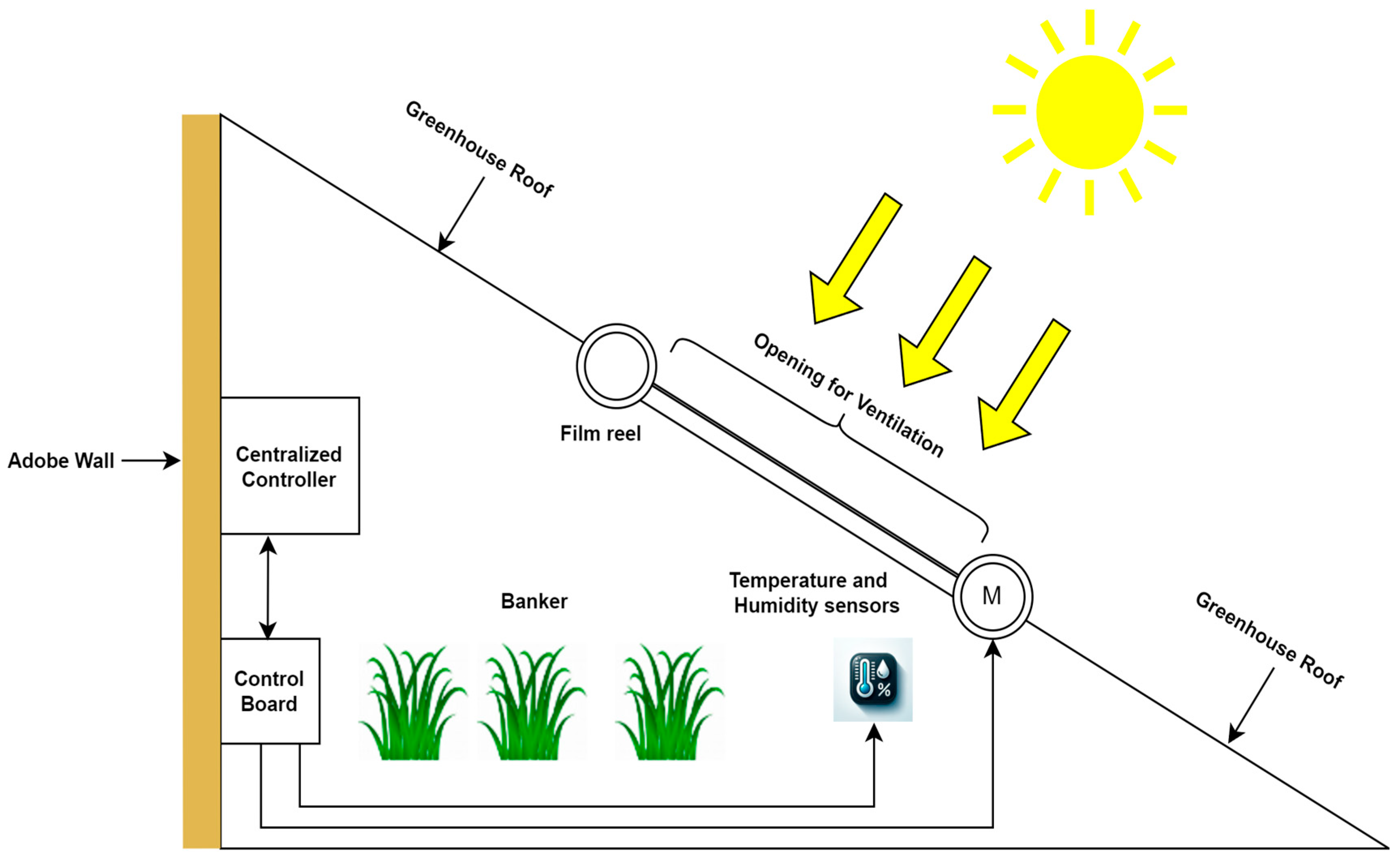
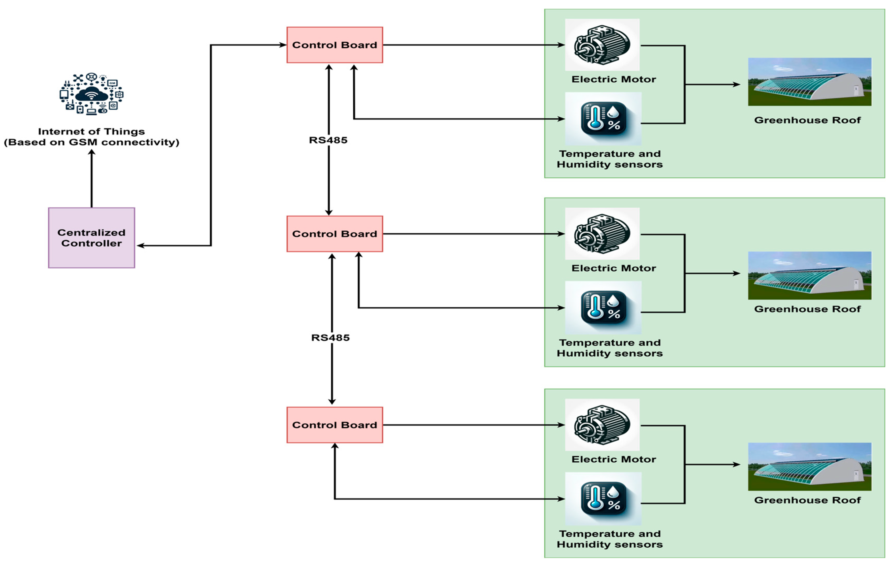
2. System Overview
3. Algorithm Design
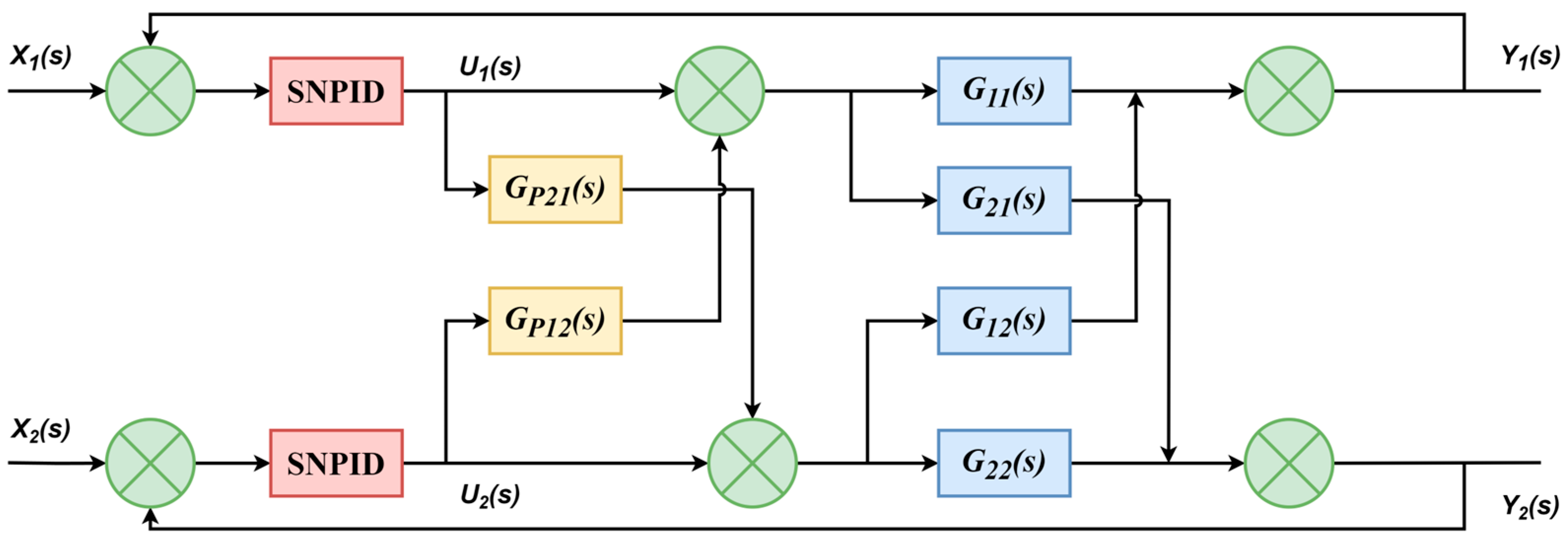
3.1. Temperature and Humidity Decoupling Control Method
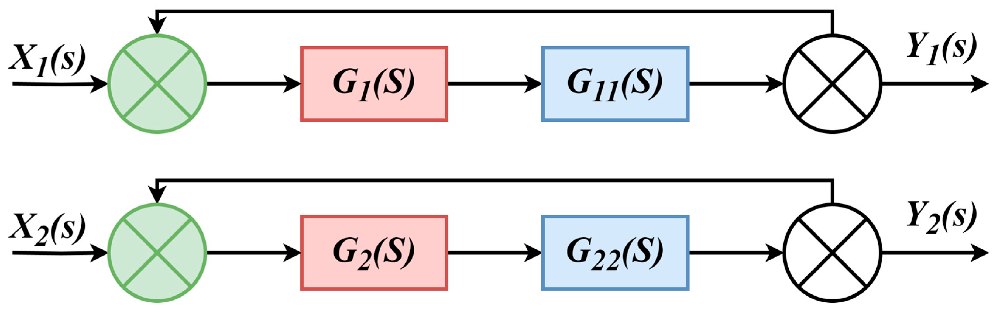
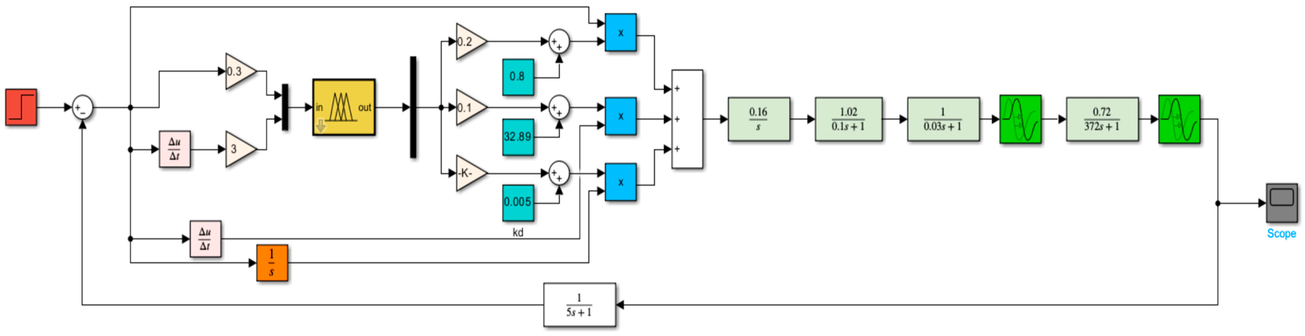
3.1.1. Decoupler Design
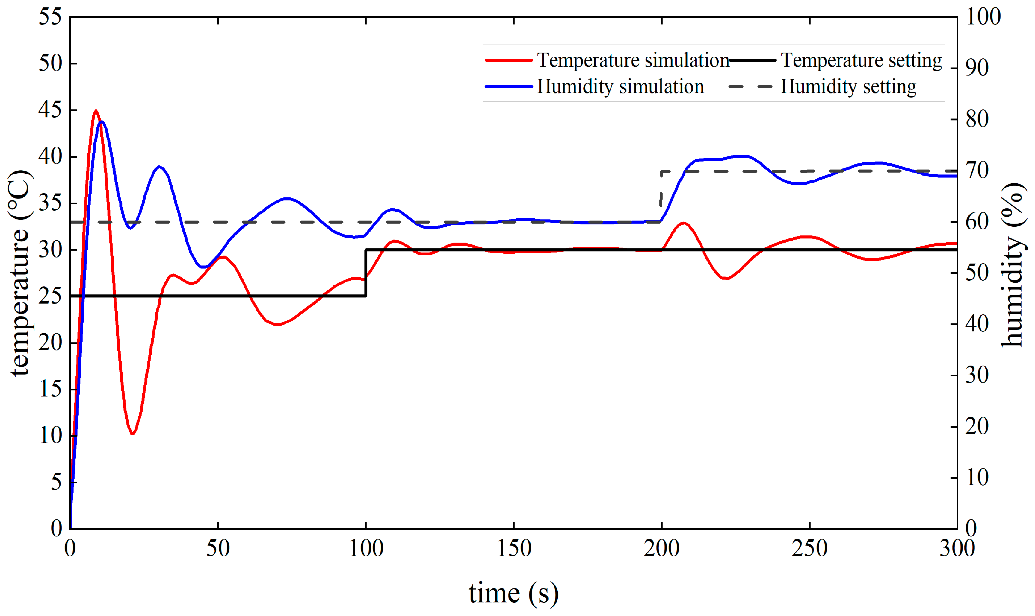
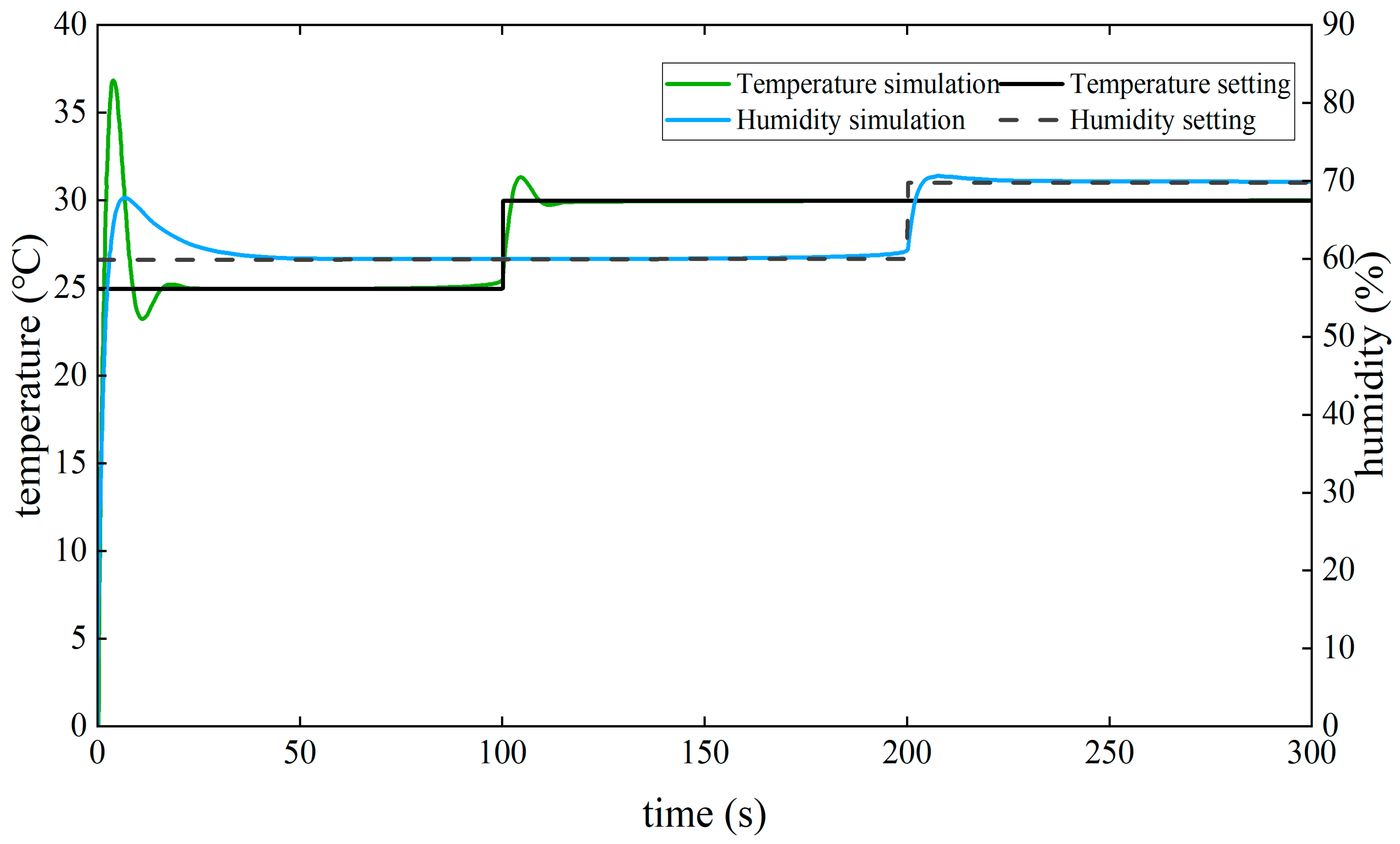
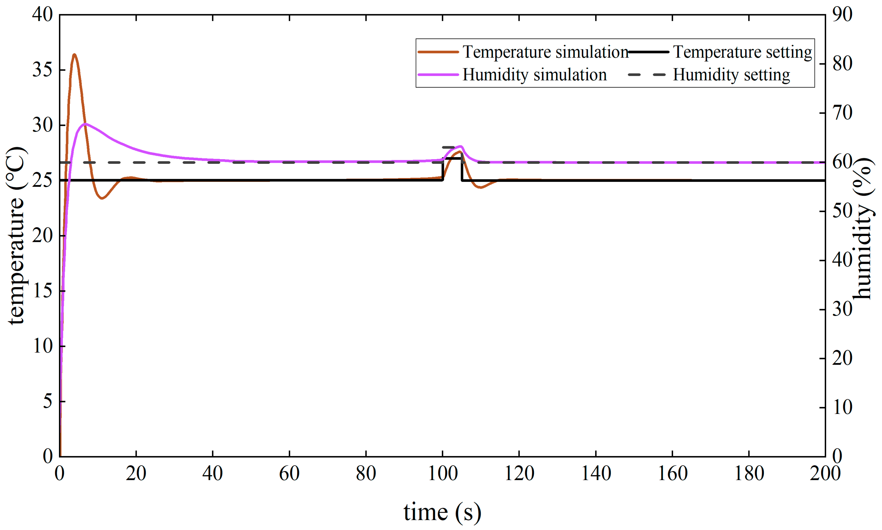
3.1.2. Simulation Experiments and Results Analysis
- (1)
- Undecoupled dynamic test
- (2)
- Dynamic test
- (3)
- Perturbation experiments
3.2. Adaptive Fuzzy PID Controller Settings
3.2.1. Overview of Traditional PID
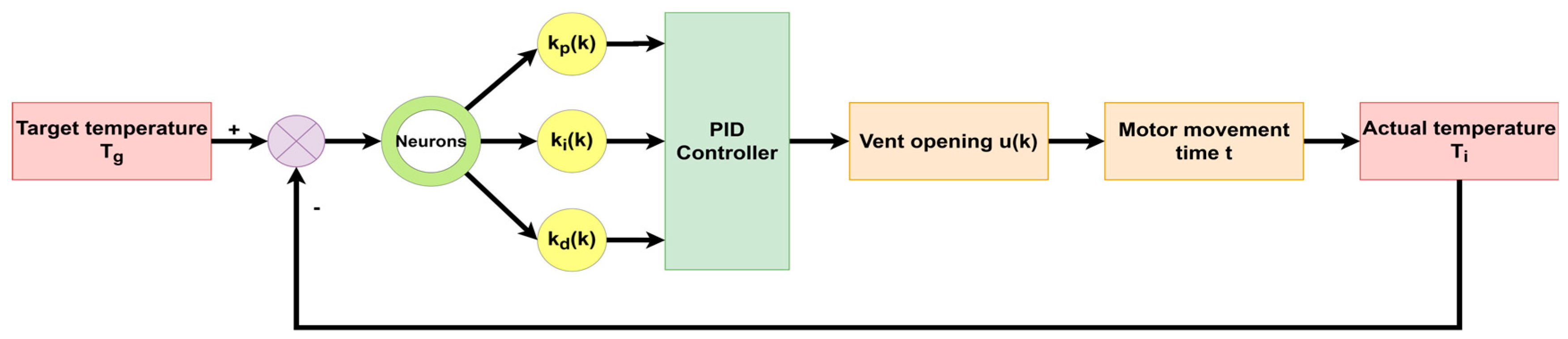
3.2.2. Control System Structure
3.2.3. Control Principle
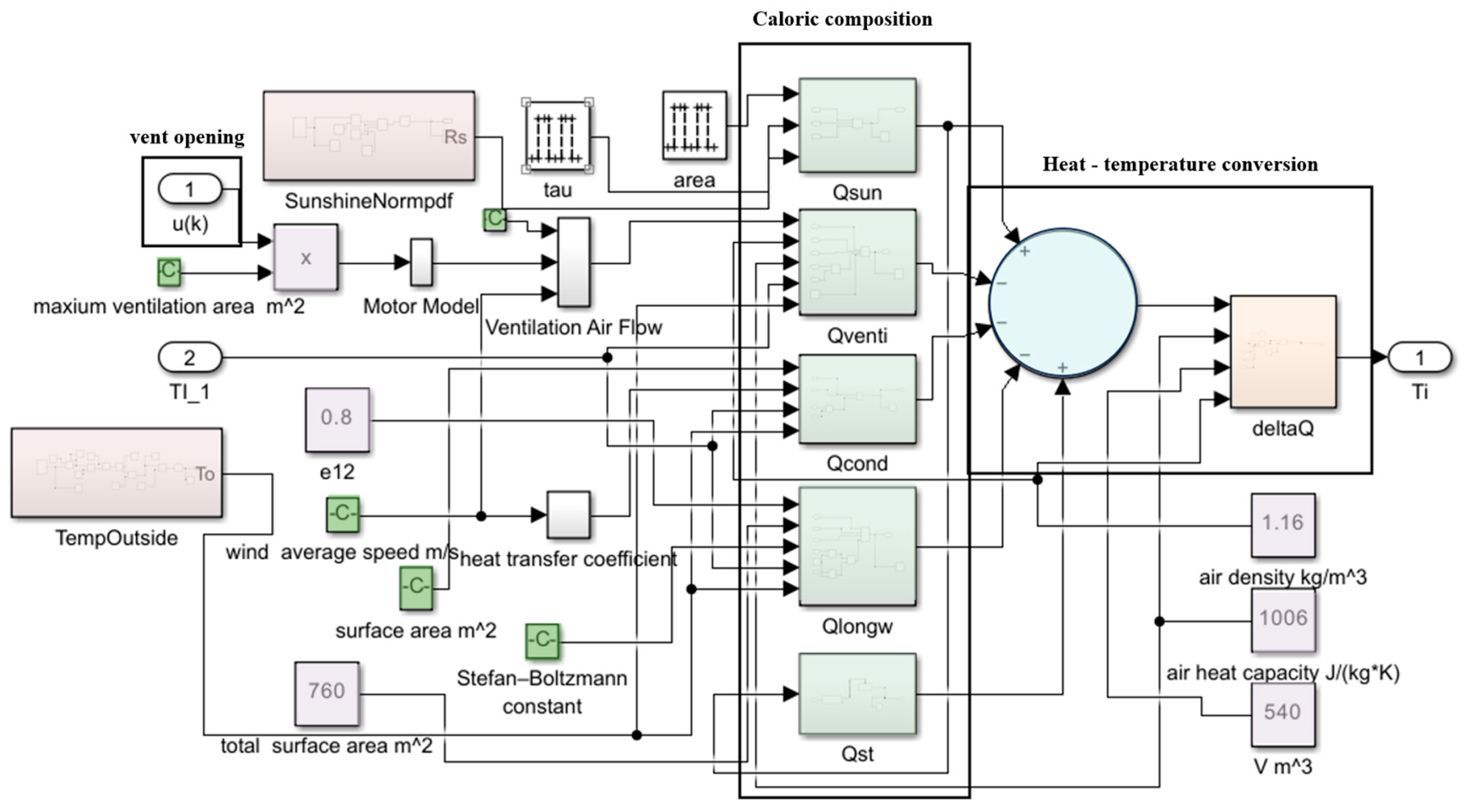
3.2.4. Model Building
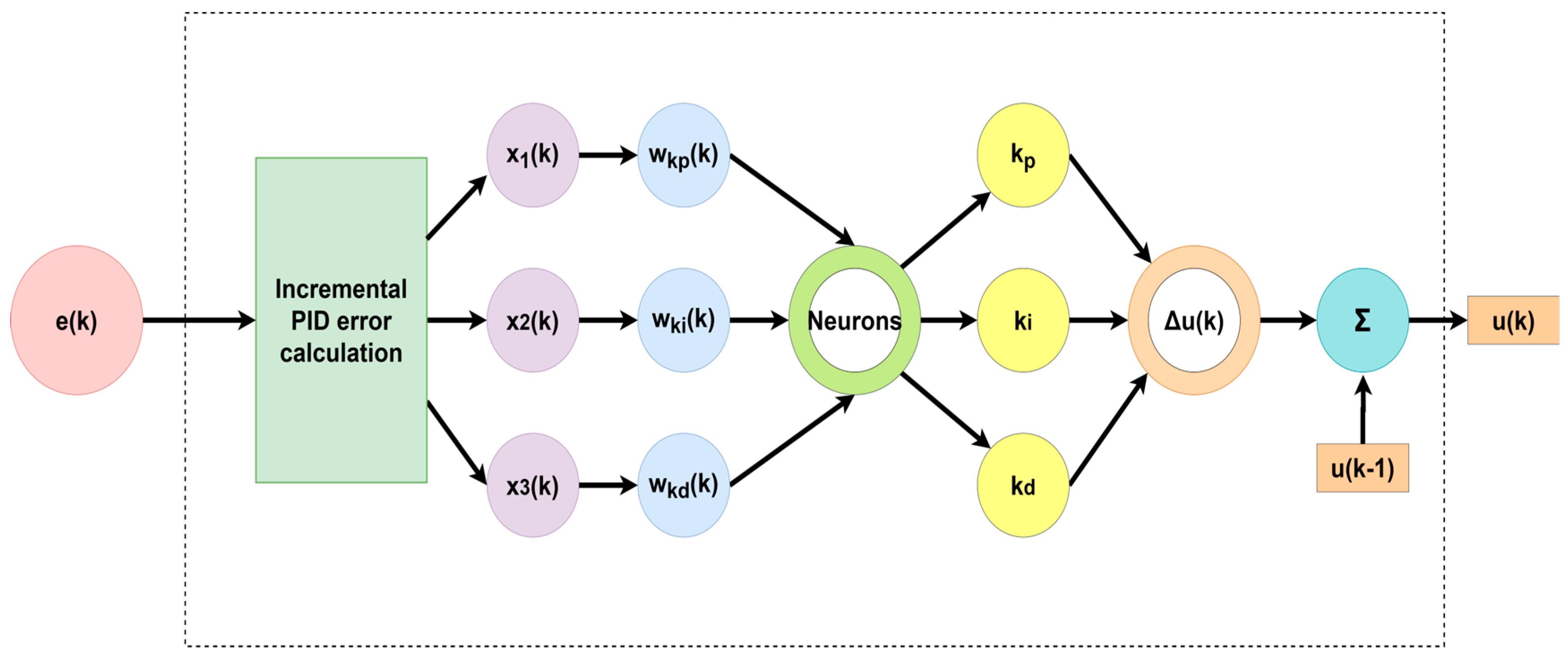
3.3. Design of SNPID Controller
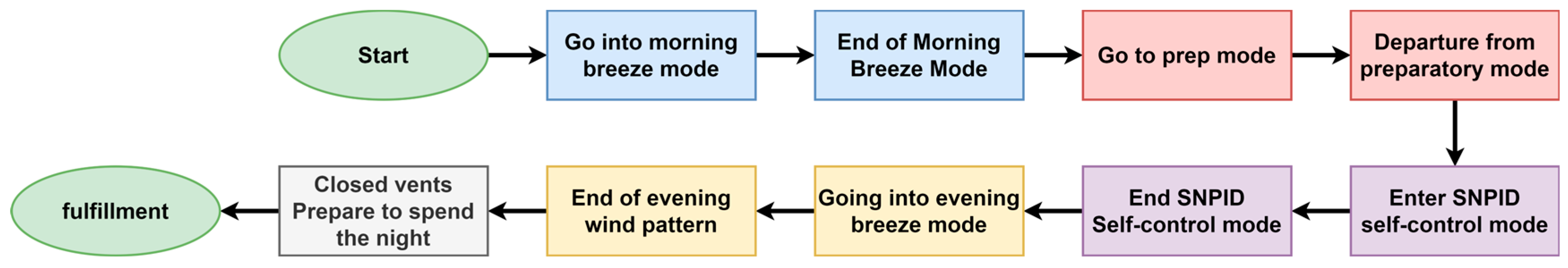
3.4. Temperature and Humidity Control Algorithm Design
4. Algorithm Deployment on Hardware Platforms
4.1. Migration and Implementation of the Runtime Environment
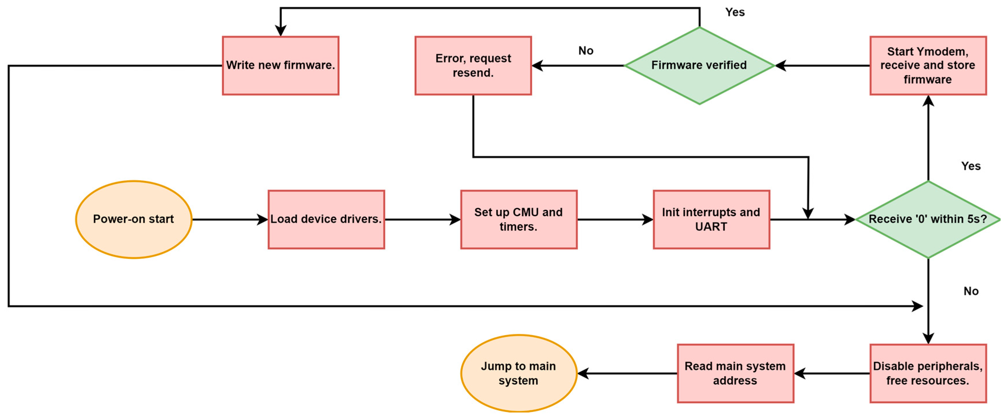
4.1.1. Bootloader Program Design and Implementation
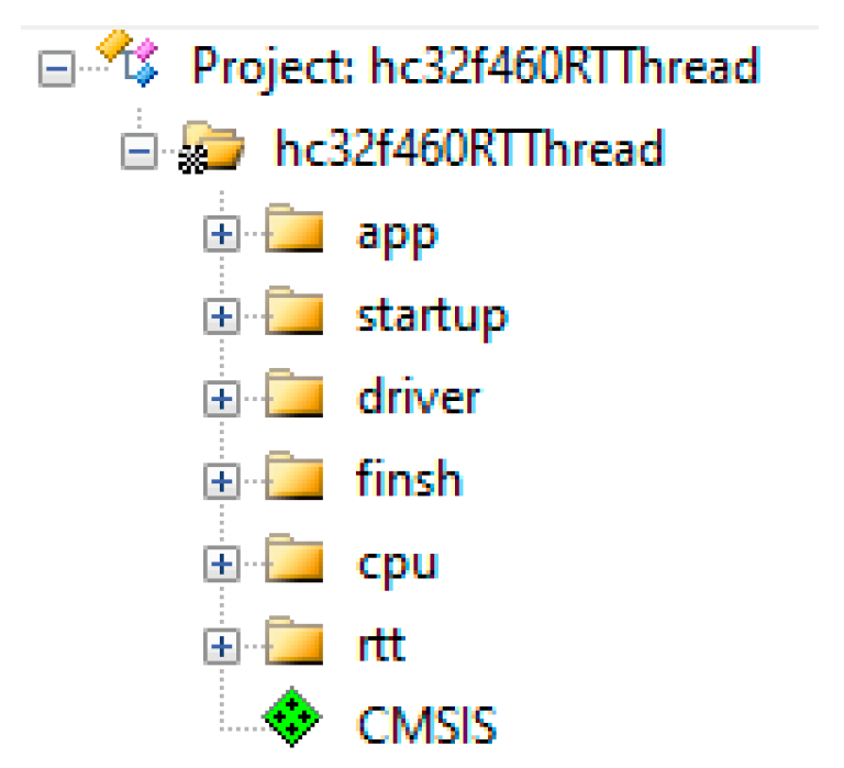
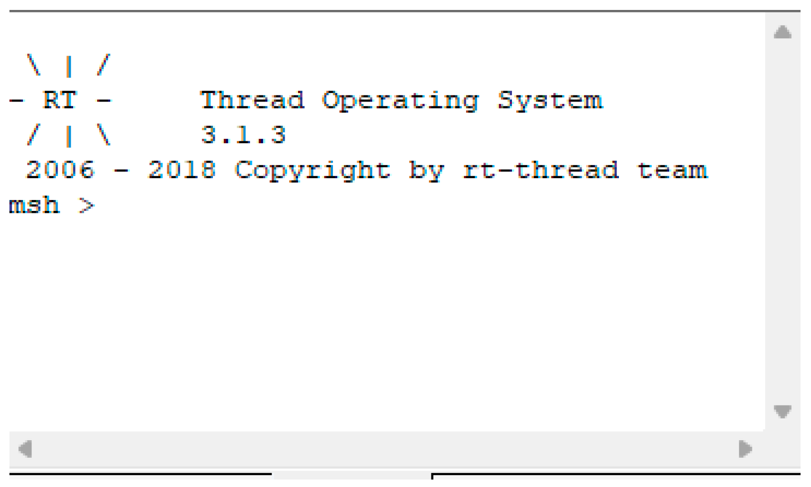
4.1.2. Tsraide’s Real-Time System Porting
4.2. Control System Software and Hardware Architecture Design
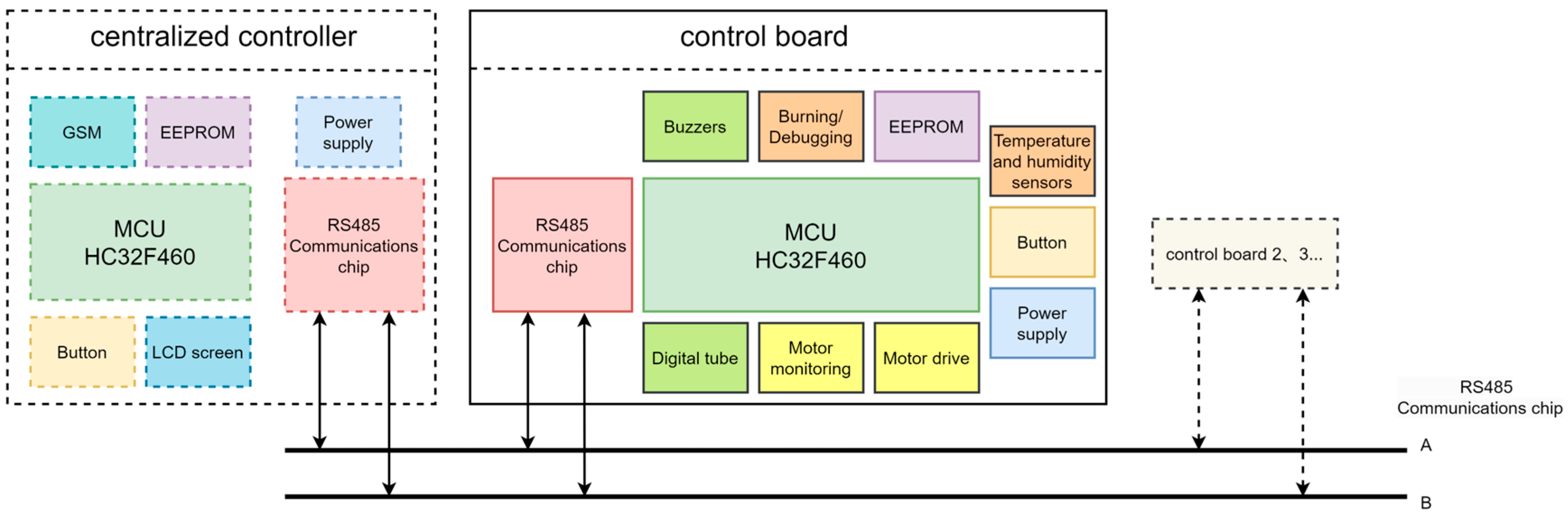
4.2.1. Overall Hardware Design
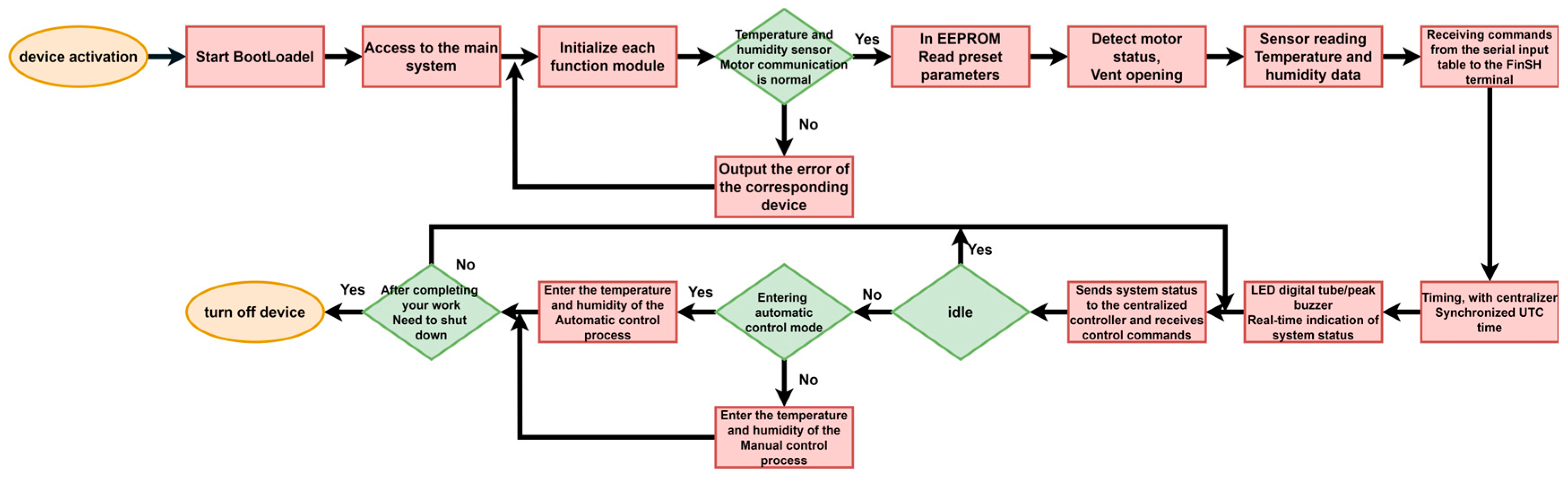
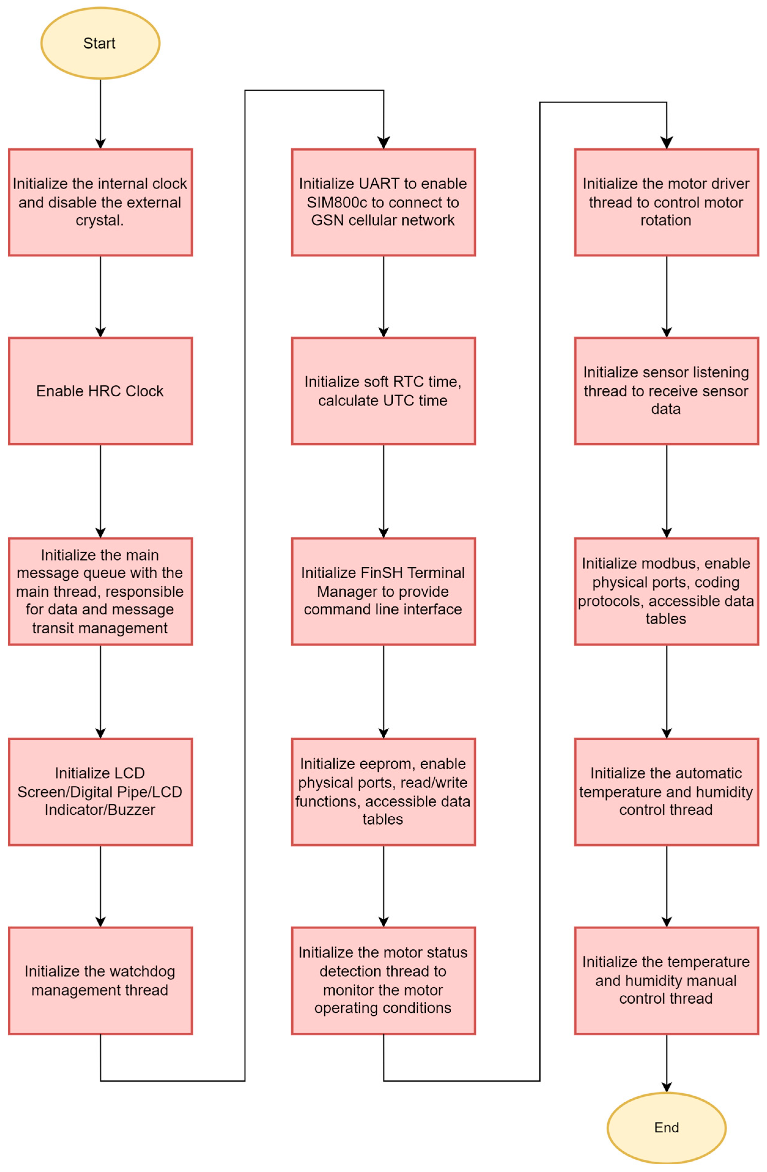
4.2.2. Main Control Board Program Process Design
4.2.3. Design and Implementation of Thread Time Slices and Interrupt Priority Tables
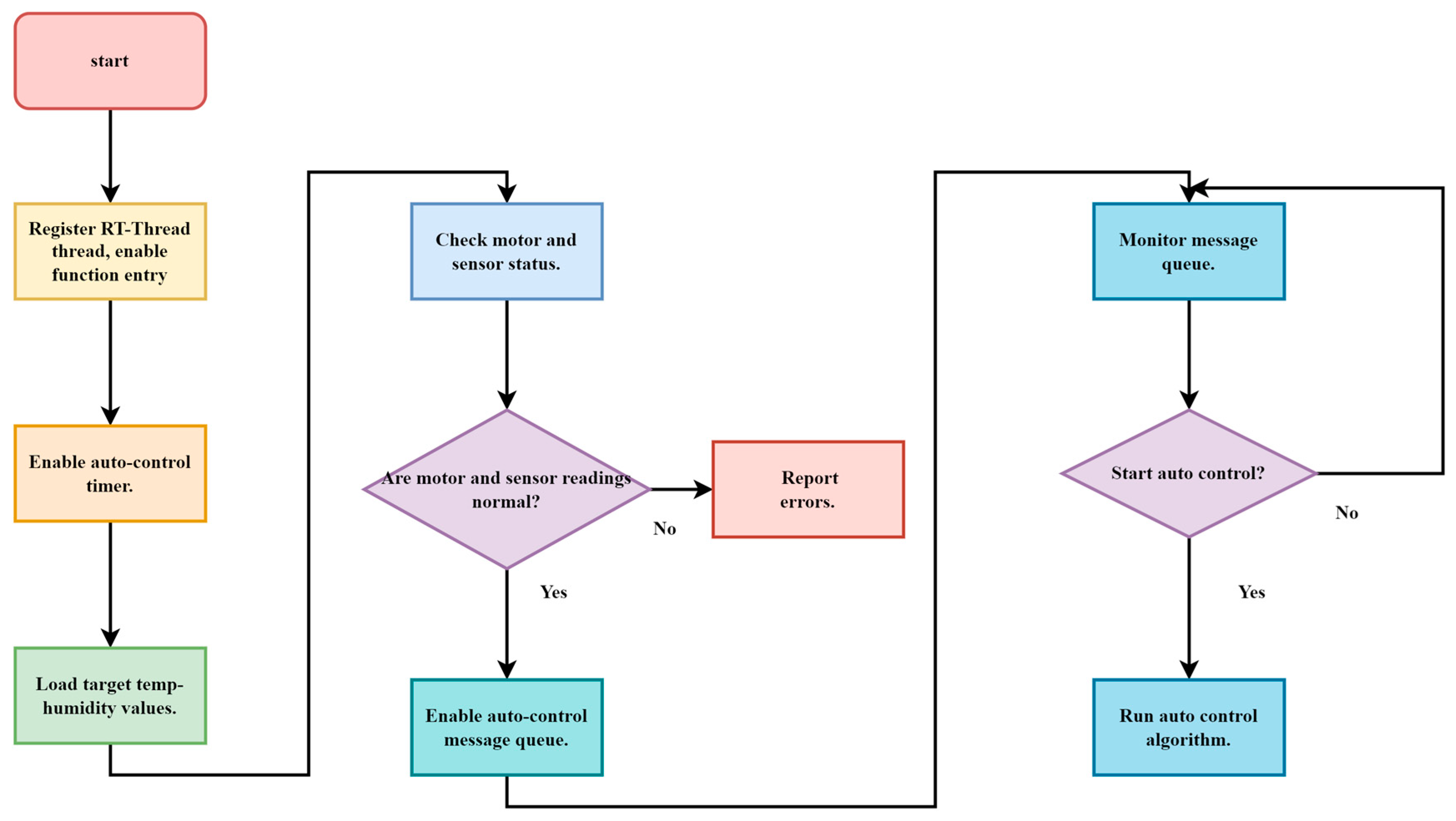
4.2.4. Automatic Temperature and Humidity Control Module
5. System Testing and Discussion of Results
5.1. Temperature Control Testing Based on Simulation Modeling
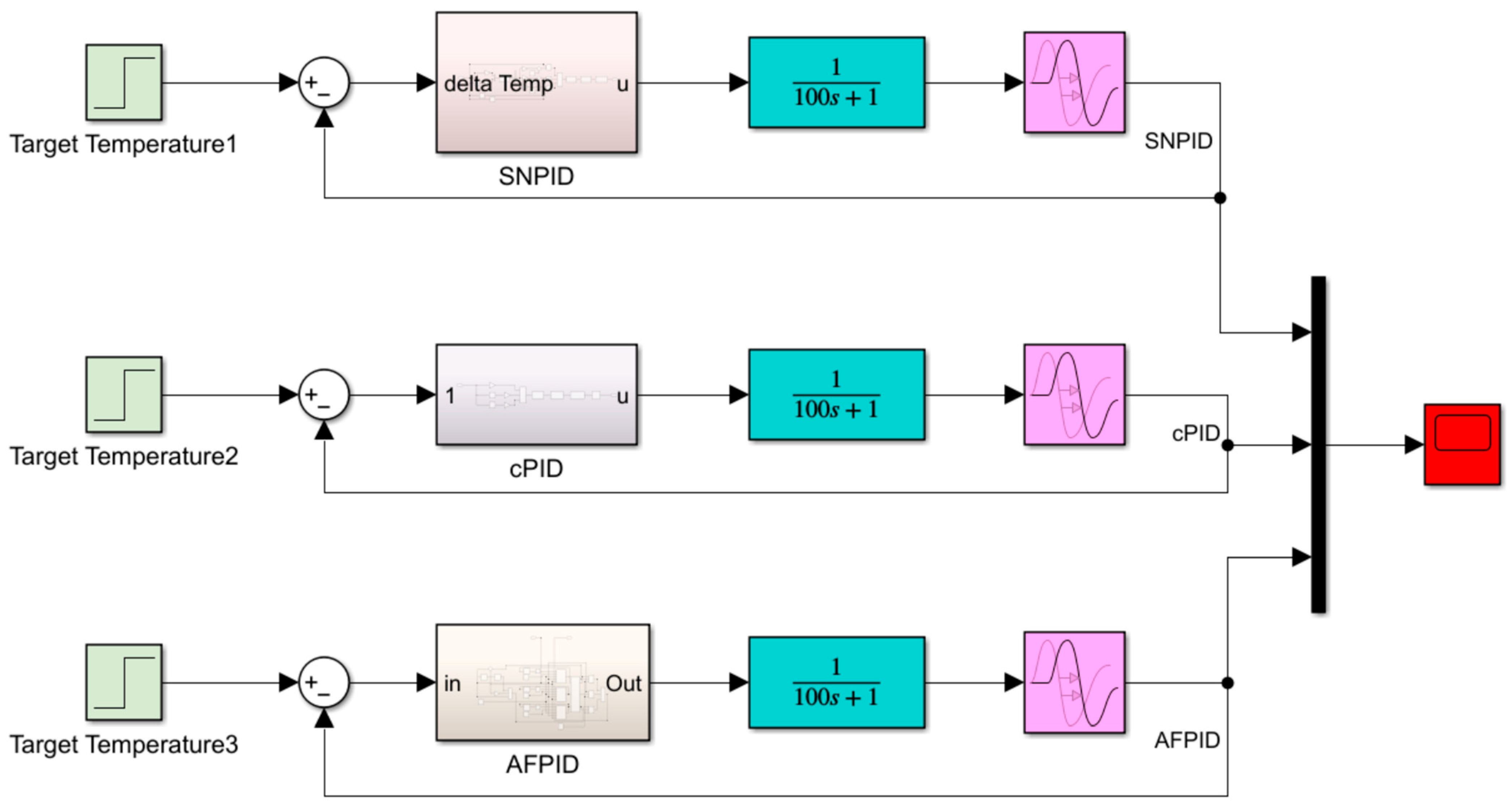
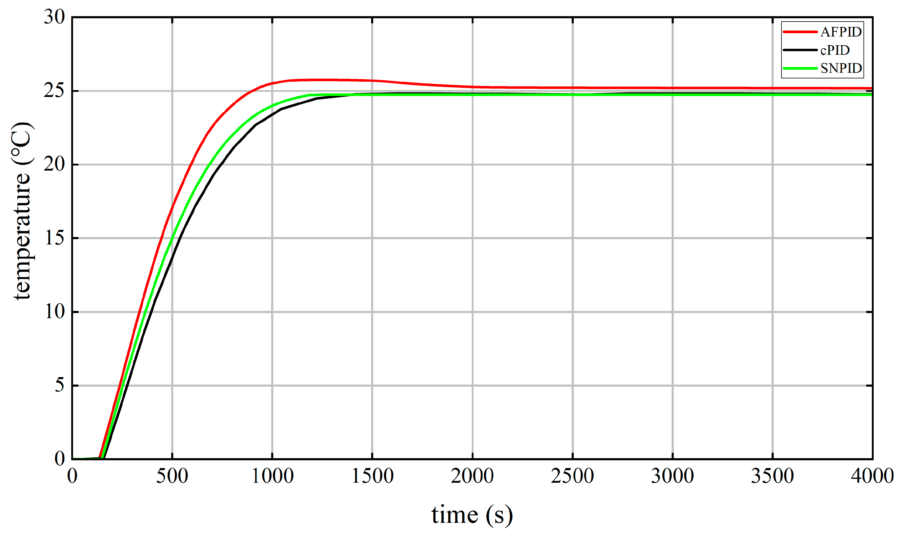
5.1.1. Step Response Performance Test of SNPID Algorithm
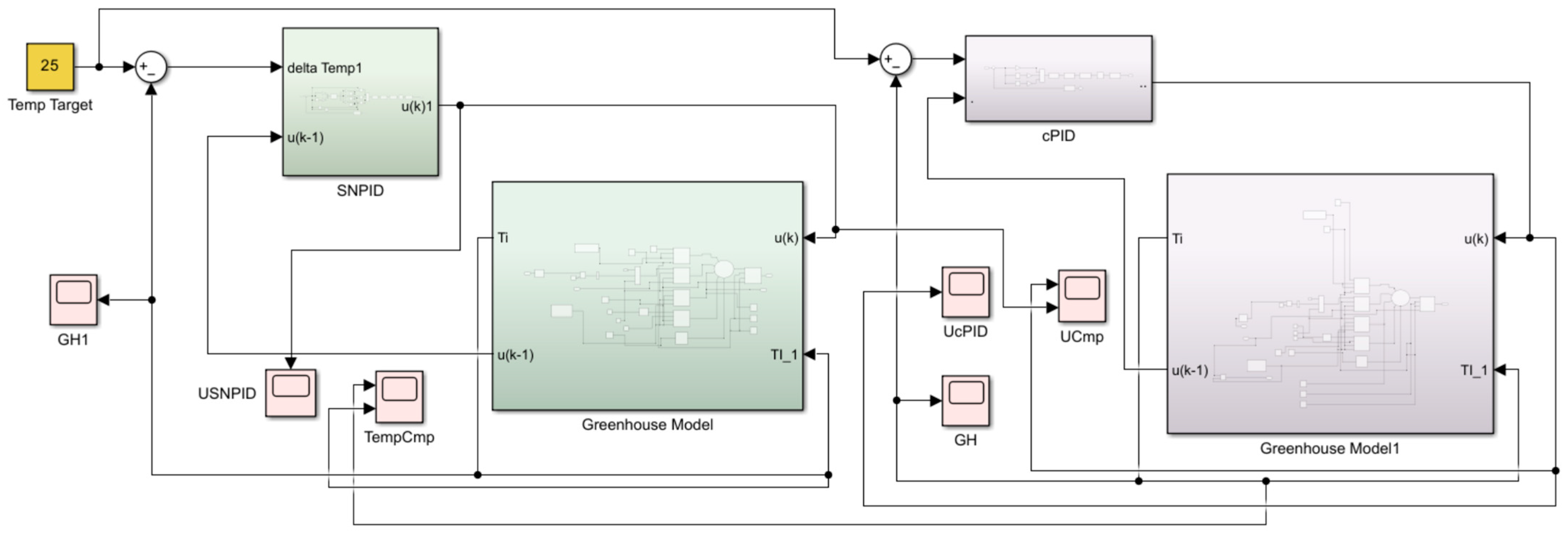
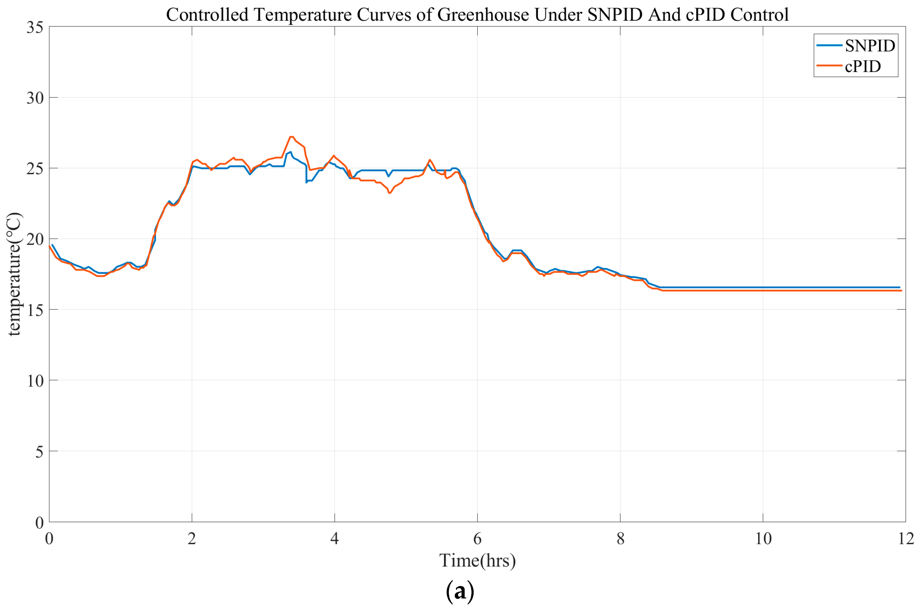
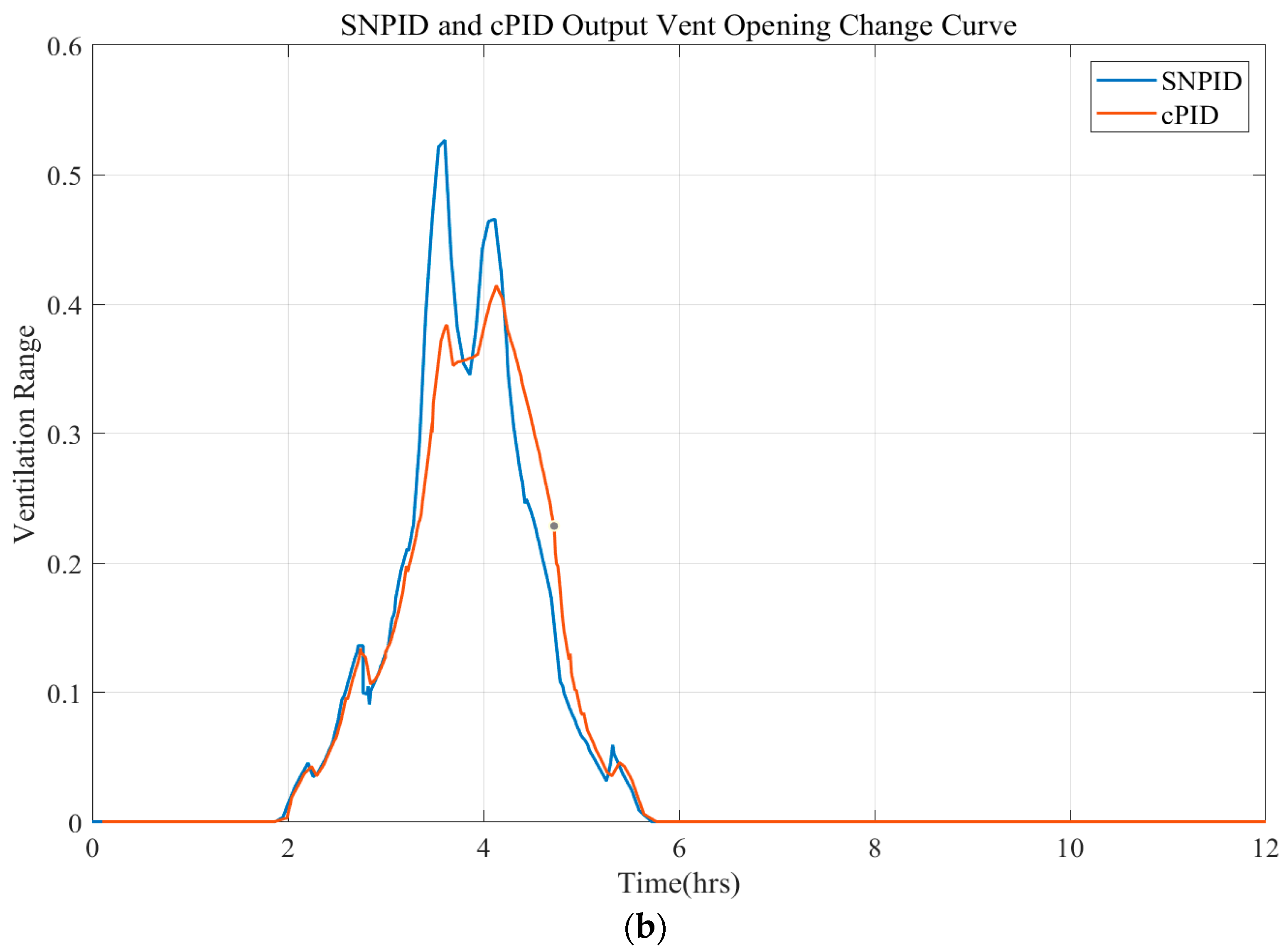
5.1.2. Simulation Tests of Controlled Temperature Profiles of Greenhouse Models
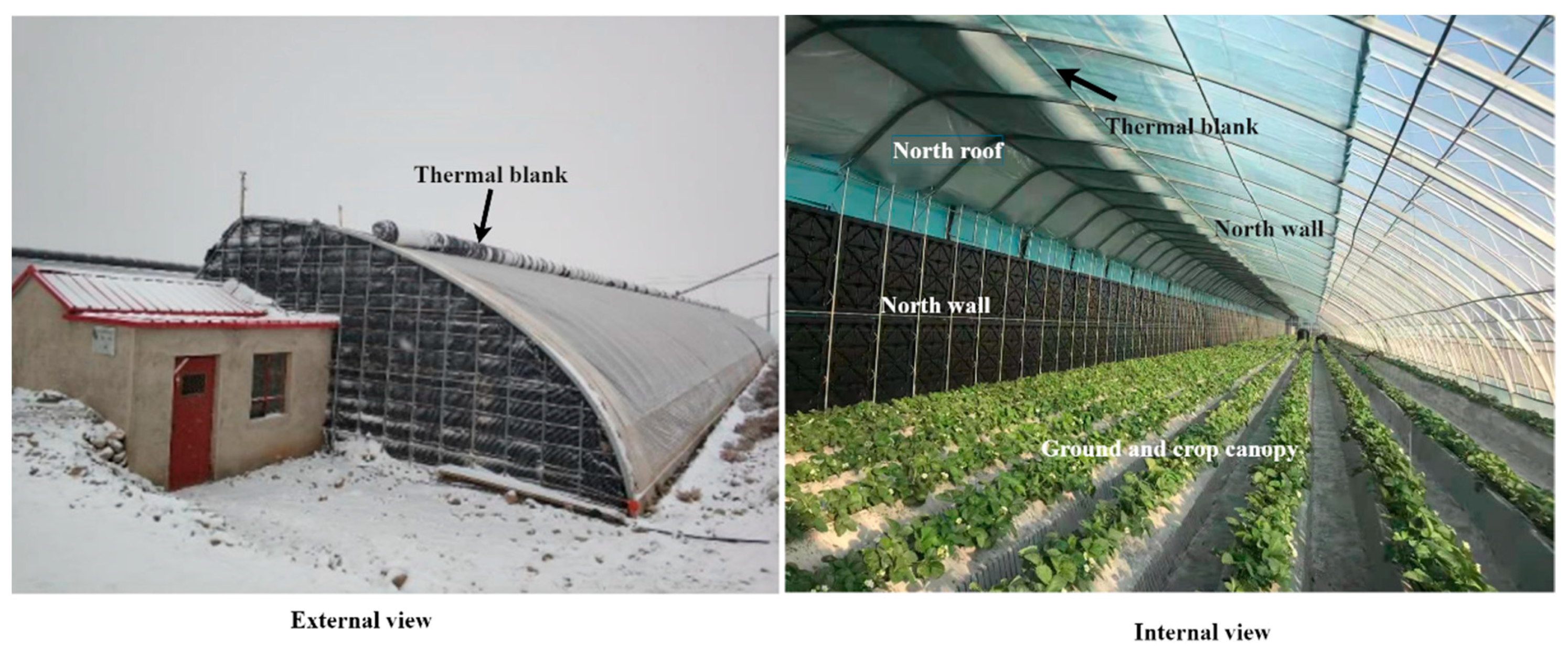
5.2. Control System Testing Based on Real Greenhouses
5.2.1. Main Control Board Function Test
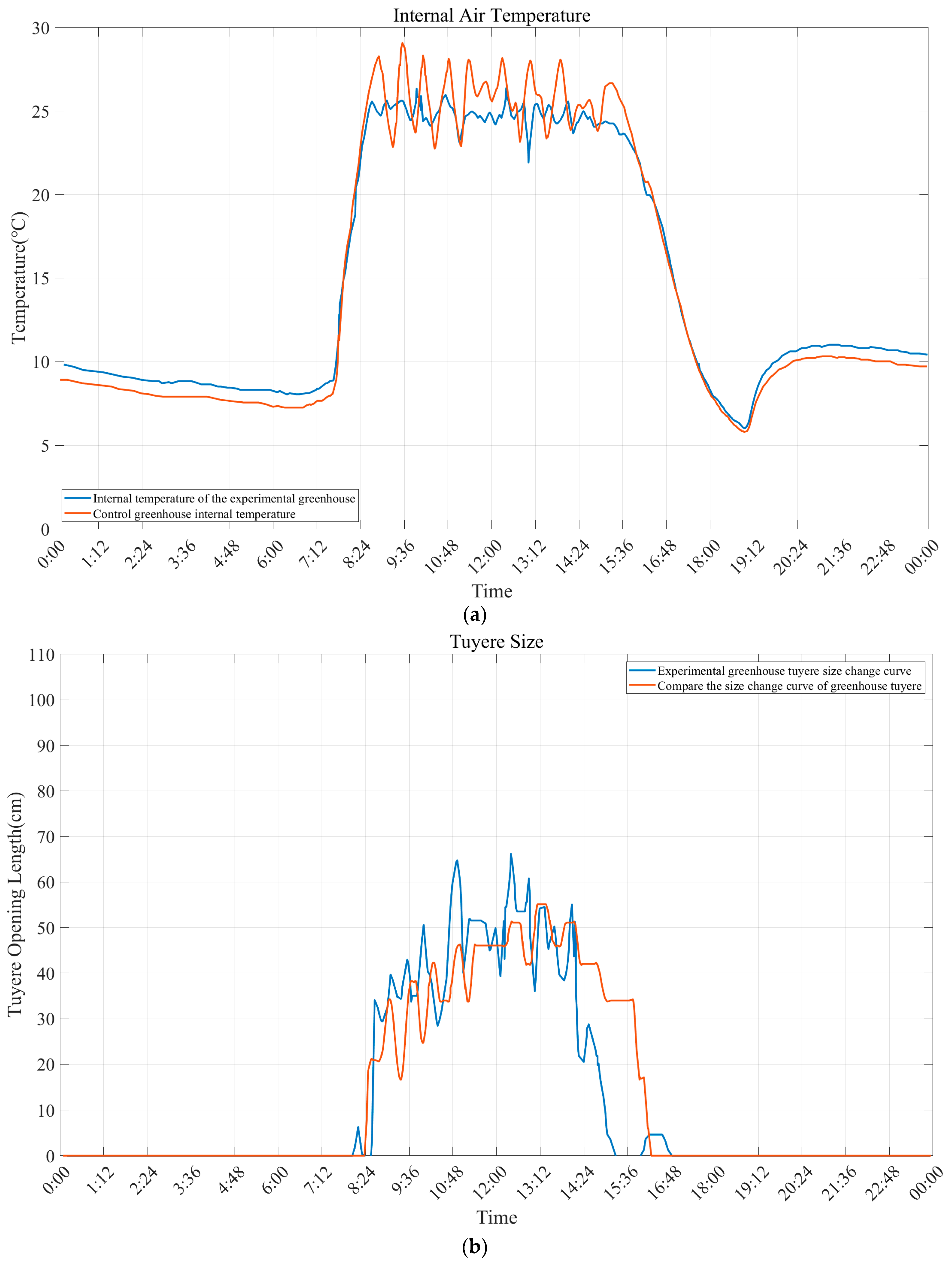
5.2.2. Temperature and Humidity Control Effect Test
- A.
- Testing the effectiveness of air temperature control in chambers
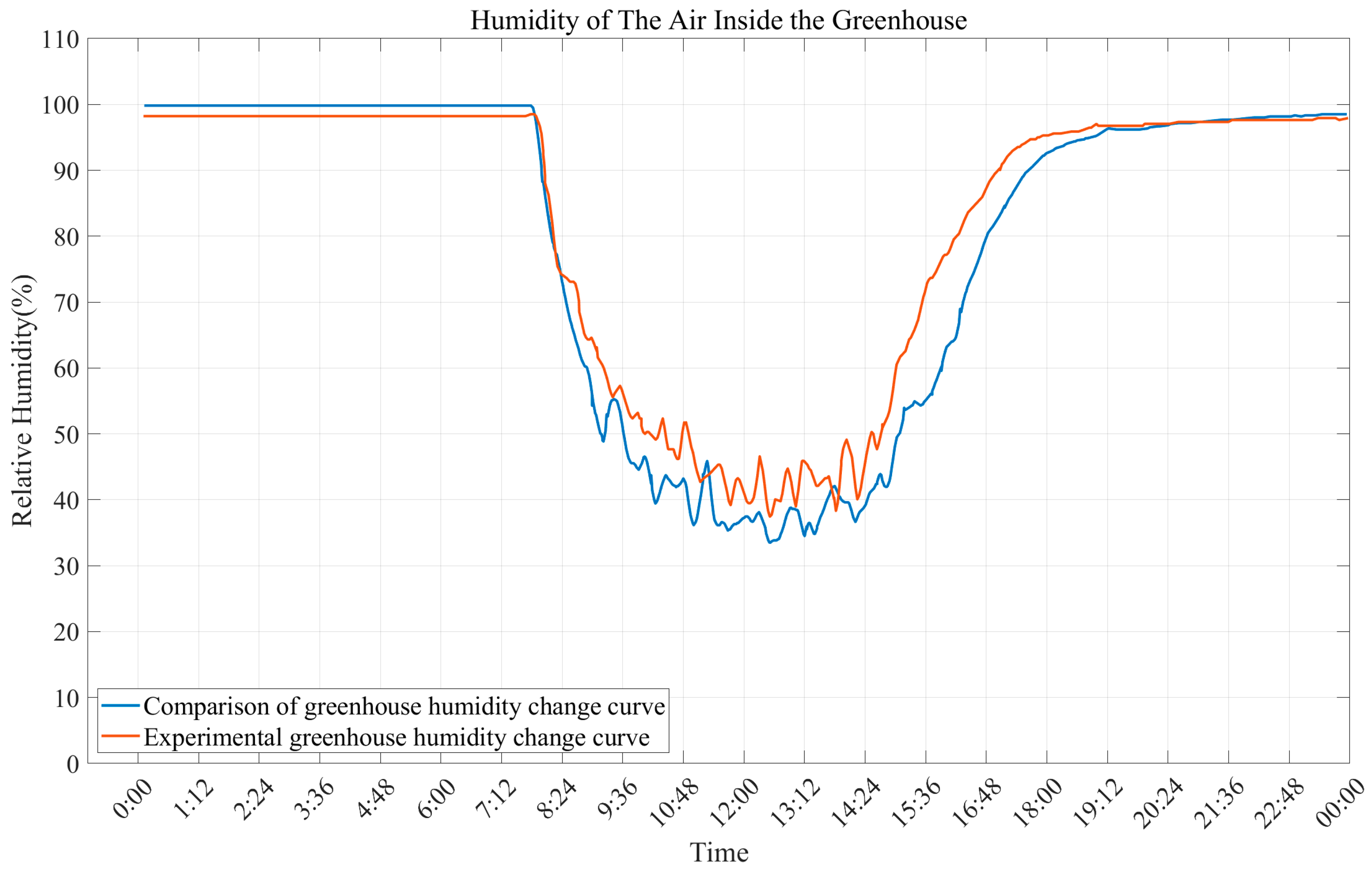
- B.
- Testing the effectiveness of air humidity control in chambers
6. Conclusions
Supplementary Materials
Author Contributions
Funding
Data Availability Statement
Conflicts of Interest
References
- Ravishankar, E.; Booth, R.E.; Hollingsworth, J.A.; Ade, H.; Sederoff, H.; DeCarolis, J.F.; O’Connor, B.T. Organic solar powered greenhouse performance optimization and global economic opportunity. Energy Environ. Sci. 2022, 15, 1659–1671. [Google Scholar] [CrossRef]
- Zhang, X.; Lv, J.; Xie, J.; Yu, J.; Zhang, J.; Tang, C.; Li, J.; He, Z.; Wang, C. Solar radiation allocation and spatial distribution in chinese solar greenhouses: Model development and application. Energies 2020, 13, 1108. [Google Scholar] [CrossRef]
- Zhang, Y.; Henke, M.; Li, Y.; Xu, D.; Liu, A.; Liu, X.; Li, T. Towards the maximization of energy performance of an energy-saving Chinese solar greenhouse: A systematic analysis of common greenhouse shapes. Sol. Energy 2022, 236, 320–334. [Google Scholar] [CrossRef]
- Yau, J.; Wei, J.J.; Wang, H.; Eniola, O.; Ibitoye, F.P. Modeling of the internal temperature for an energy saving Chinese solar greenhouse. Eng. Technol. Appl. Sci. Res. 2020, 10, 6276–6281. [Google Scholar] [CrossRef]
- Zhang, L.; Liu, X.; Shi, W.; Li, T.; Ji, J. Study of a novel front-roof-back natural ventilation system for Chinese solar greenhouses. R. Soc. Open Sci. 2022, 9, 220251. [Google Scholar] [CrossRef] [PubMed]
- Kang, M.; Fan, X.-R.; Hua, J.; Wang, H.; Wang, X.; Wang, F.-Y. Managing traditional solar greenhouse with CPSS: A just-for-fit philosophy. IEEE Trans. Cybern. 2018, 48, 3371–3380. [Google Scholar] [CrossRef] [PubMed]
- Li, Z.; Yano, A.; Cossu, M.; Yoshioka, H.; Kita, I.; Ibaraki, Y. Electrical energy producing greenhouse shading system with a semi-transparent photovoltaic blind based on micro-spherical solar cells. Energies 2018, 11, 1681. [Google Scholar] [CrossRef]
- Yun, J.-W.; Lee, D.-S.; Kim, S.-S. Analysis on productivity and efficiency of greenhouse rose farming. J. Korea Acad. Ind. Coop. Soc. 2020, 21, 532–542. [Google Scholar]
- Fokui, W.S.T.; Saulo, M.; Ngoo, L. Climate Change Mitigation in Cities by Adopting Solar Streetlights with Energy Management Capabilities: Case of Nairobi. In Proceedings of the 2022 IEEE 21st Mediterranean Electrotechnical Conference (MELECON), Palermo, Italy, 14–16 June 2022; pp. 390–395. [Google Scholar]
- Ding, D. Integration of Active Solar Thermal Technologies in Greenhouses: A Mini Review. Front. Energy Res. 2021, 9, 757553. [Google Scholar] [CrossRef]
- Nouadjep, S.N.; Djouodjinang, H.F. IoT and Arduino Based Design of a Solar, Automated and Smart Greenhouse for Vegetable. E3S Web Conf. 2022, 354, 01002. [Google Scholar] [CrossRef]
- Suji Prasad, S.; Thangatamilan, M.; Suresh, M.; Panchal, H.; Rajan, C.A.; Sagana, C.; Gunapriya, B.; Sharma, A.; Panchal, T.; Sadasivuni, K.K. An efficient LoRa-based smart agriculture management and monitoring system using wireless sensor networks. Int. J. Ambient Energy 2022, 43, 5447–5450. [Google Scholar] [CrossRef]
- Ahmad, B.; Ahmed, R.; Masroor, S.; Mahmood, B.; Hasan, S.Z.U.; Jamil, M.; Khan, M.T.; Younas, M.T.; Wahab, A.; Haydar, B.; et al. Evaluation of smart greenhouse monitoring system using raspberry-pi microcontroller for the production of tomato crop. J. Appl. Res. Plant Sci. 2023, 4, 452–458. [Google Scholar] [CrossRef]
- Wei, X. Intelligent temperature control system of greenhouse based on STM32 single chip microcomputer. J. Phys. Conf. Ser. 2022, 2254, 012046. [Google Scholar] [CrossRef]
- Abbood, H.M.; Nouri, N.; Riahi, M.; Alagheband, S.H. An intelligent monitoring model for greenhouse microclimate based on RBF Neural Network for optimal setpoint detection. J. Process. Control 2023, 129, 103037. [Google Scholar] [CrossRef]
- Cheng, Y. Research on intelligent control of an agricultural greenhouse based on fuzzy PID control. J. Environ. Eng. Sci. 2020, 15, 113–118. [Google Scholar] [CrossRef]
- Wang, Y.; Lu, Y.; Xiao, R. Application of Nonlinear Adaptive Control in Temperature of Chinese Solar Greenhouses. Electronics 2021, 10, 1582. [Google Scholar] [CrossRef]
- Wang, Y.; Wang, Z.; Zhang, H.; Xie, X. Finite-time adaptive fuzzy event-triggered control for nonstrict feedback stochastic nonlinear systems with multiple constraints. IEEE Trans. Fuzzy Syst. 2023, 31, 3896–3905. [Google Scholar] [CrossRef]
- Yuan, Y.; Zhao, J.; Sun, Z.-Y.; Xie, X. Practically fast finite-time stability in the mean square of stochastic nonlinear systems: Application to one-link manipulator. IEEE Trans. Syst. Man, Cybern. Syst. 2023, 54, 312–323. [Google Scholar] [CrossRef]
- Xia, J.; Li, B.; Su, S.-F.; Sun, W.; Shen, H. Finite-time command filtered event-triggered adaptive fuzzy tracking control for stochastic nonlinear systems. IEEE Trans. Fuzzy Syst. 2020, 29, 1815–1825. [Google Scholar] [CrossRef]
- Sun, K.; Qiu, J.; Karimi, H.R.; Fu, Y. Event-triggered robust fuzzy adaptive finite-time control of nonlinear systems with pre-scribed performance. IEEE Trans. Fuzzy Syst. 2020, 29, 1460–1471. [Google Scholar] [CrossRef]
- Wu, Y.; Zhang, G.; Wu, L.-B. Finite-time adaptive fuzzy switching event-triggered control for nonaffine stochastic systems. IEEE Trans. Fuzzy Syst. 2022, 30, 5261–5275. [Google Scholar] [CrossRef]
- Sui, S.; Chen, C.P.; Tong, S. Event-trigger-based finite-time fuzzy adaptive control for stochastic nonlinear system with un-modeled dynamics. IEEE Trans. Fuzzy Syst. 2020, 29, 1914–1926. [Google Scholar] [CrossRef]
- Zhou, H.; Sui, S.; Tong, S. Fuzzy adaptive finite-time consensus control for high-order nonlinear multiagent systems based on event-triggered. IEEE Trans. Fuzzy Syst. 2022, 30, 4891–4904. [Google Scholar] [CrossRef]
- Li, Y.-X.; Yang, G.-H. Observer-based fuzzy adaptive event-triggered control codesign for a class of uncertain nonlinear systems. IEEE Trans. Fuzzy Syst. 2017, 26, 1589–1599. [Google Scholar] [CrossRef]
- Ma, H.; Li, H.; Liang, H.; Dong, G. Adaptive fuzzy event-triggered control for stochastic nonlinear systems with full state constraints and actuator faults. IEEE Trans. Fuzzy Syst. 2019, 27, 2242–2254. [Google Scholar] [CrossRef]
- Wu, R.; Yu, K.; Li, Y. Adaptive Fuzzy 1-Bit Event-Triggered Control for Stochastic Nonlinear Systems. In Proceedings of the 2021 13th International Conference on Advanced Computational Intelligence (ICACI), Wanzhou, China, 14–16 May 2021; pp. 68–73. [Google Scholar]
- Zhang, R.-Y.; Wu, L.-B.; Zhao, N.-N.; Yan, Y. Adaptive event-triggered fuzzy tracking control of uncertain stochastic nonlinear systems with unmeasurable states. IEEE Trans. Fuzzy Syst. 2021, 30, 2183–2196. [Google Scholar] [CrossRef]
- Yang, W.; Zheng, W.X.; Yu, W. Observer-based event-triggered adaptive fuzzy control for fractional-order time-varying delayed MIMO systems against actuator faults. IEEE Trans. Fuzzy Syst. 2022, 30, 5445–5459. [Google Scholar] [CrossRef]
- Liu, Y.; Zhang, H.; Sun, J.; Wang, Y. Event-triggered adaptive finite-time containment control for fractional-order nonlinear multiagent systems. IEEE Trans. Cybern. 2022, 54, 1250–1260. [Google Scholar] [CrossRef] [PubMed]
- Chen, T.; Yang, H.; Yuan, J. Event-triggered adaptive neural network backstepping sliding mode control for fractional order chaotic systems synchronization with input delay. IEEE Access 2021, 9, 100868–100881. [Google Scholar] [CrossRef]
- Jia, Y. Design of an intelligent greenhouse remote control system based on a fuzzy neural network. Int. J. Autom. Technol. 2021, 15, 243–248. [Google Scholar] [CrossRef]
- Qun, R. Intelligent control technology of agricultural greenhouse operation robot based on fuzzy PID path tracking algorithm. INMATEH Agric. Eng. 2020, 62, 181–190. [Google Scholar] [CrossRef]
- Elanchezhian, A.; Basak, J.; Park, J.; Khan, F.; Okyere, F.; Lee, Y.; Bhujel, A.; Lee, D.; Sihalath, T.; Kim, H. Evaluating different models used for predicting the indoor microclimatic parameters of a greenhouse. Appl. Ecol. Environ. Res. 2020, 18, 2141–2161. [Google Scholar] [CrossRef]
- Yao, Y.; Tan, J.; Wu, J. Finite-time tracking control for nonstrict-feedback state-delayed nonlinear systems with full-state constraints and unmodeled dynamics. Complexity 2020, 2020, 8887925. [Google Scholar] [CrossRef]
- Hou, Y.; Xu, X.; Liu, R.; Bai, X.; Liu, H. Adaptive finite-time fuzzy control for uncertain nonlinear systems with asymmetric full-state constraints. Mathematics 2023, 11, 4313. [Google Scholar] [CrossRef]
- Ungurean, I. Timing Comparison of the real-time operating systems for small microcontrollers. Symmetry 2020, 12, 592. [Google Scholar] [CrossRef]
- Xie, X.; Ye, J.; Wu, L.; Li, R. RTOSExtracter: Extracting user-defined functions in stripped RTOS-based firmware. In Proceedings of the 2022 International Conference on Cyber-Enabled Distributed Computing and Knowledge Discovery (CyberC), Suzhou, China, 14–16 October 2022; pp. 87–96. [Google Scholar]
- Zhang, H.; Yang, L. Position and attitude control based on single neuron pid with gravity compensation for quad rotor UAV. J. Aerosp. Technol. Manag. 2023, 15, e1023. [Google Scholar] [CrossRef]
- Li, Y.; Dong, Y.; Fan, P. Positioning Control of Piezoelectric Stick-slip Actuators Based on Single Neuron Adaptive PID Algo-rithm. In Proceedings of the 2021 11th International Conference on Intelligent Control and Information Processing (ICICIP), Dali, China, 3–7 December 2021; pp. 227–234. [Google Scholar]
- Su, D.; Yao, W.; Yu, F.; Liu, Y.; Zheng, Z.; Wang, Y.; Xu, T.; Chen, C. Single-neuron PID UAV variable fertilizer application control system based on a weighted coefficient learning correction. Agriculture 2022, 12, 1019. [Google Scholar] [CrossRef]
- Zhiqi, Y. Application of Improved PID Control Algorithm in Intelligent Vehicle. In Proceedings of the 2022 IEEE 6th Advanced Information Technology, Electronic and Automation Control Conference (IAEAC), Beijing, China, 3–5 October 2022; pp. 910–913. [Google Scholar]
- Wan, S.; Wang, K.; Xu, P.; Huang, Y. Numerical and experimental verification of the single neural adaptive PID real-time inverse method for solving inverse heat conduction problems. Int. J. Heat Mass Transf. 2022, 189, 122657. [Google Scholar] [CrossRef]
- Zhou, X.; Wang, J.; Huang, L.; Li, D.; Duan, Q. Modelling and controlling dissolved oxygen in recirculating aquaculture systems based on mechanism analysis and an adaptive PID controller. Comput. Electron. Agric. 2022, 192, 106583. [Google Scholar] [CrossRef]
- Ghany, M.A.; Shamseldin, M.A.; Ghany, A.A. A novel fuzzy self tuning technique of single neuron PID controller for brushless DC motor. In Proceedings of the 2017 Nineteenth International Middle East Power Systems Conference (MEPCON), Cairo, Egypt, 19–21 December 2017; pp. 1453–1458. [Google Scholar]
- Yu, M.; Zou, Z.; Wang, Z. Single Neuron PID Controller Based on Quadratic Optimization and its Application on pH Process Control. In Proceedings of the 2019 Chinese Control Conference (CCC), Guangzhou, China, 27–30 July 2019; pp. 2868–2873. [Google Scholar]
- Wu, Y.; Hou, B.; Zhou, G.; Yang, J.; Jun, F.; Zhang, Y. A Smooth Angle Velocity Active Return-to-Centre Control Based on Single Neuron PID Control for Electric Power Steering System. In Proceedings of the 2020 Chinese Control and Decision Conference (CCDC), Hefei, China, 22–24 August 2020; pp. 3945–3950. [Google Scholar]
- Wang, Z.; Zhang, J. Incremental PID controller-based learning rate scheduler for stochastic gradient descent. IEEE Trans. Neural Netw. Learn. Syst. 2022, 35, 7060–7071. [Google Scholar] [CrossRef]
- Cheng, Y.-M.; Liu, C.; Wu, J.; Liu, H.-M.; Lee, I.-K.; Niu, J.; Cho, J.-P.; Koo, K.-W.; Lee, M.-W.; Woo, D.-G. A back propagation neural network with double learning rate for PID controller in phase-shifted full-bridge soft-switching power supply. J. Electr. Eng. Technol. 2020, 15, 2811–2822. [Google Scholar] [CrossRef]
- Dai, M.; Zhang, Z.; Lai, X.; Lin, X.; Wang, H. PID controller-based adaptive gradient optimizer for deep neural networks. IET Control Theory Appl. 2023, 17, 2032–2037. [Google Scholar] [CrossRef]
- Kobyzev, I.; Prince, S.J.; Brubaker, M.A. Normalizing flows: An introduction and review of current methods. IEEE Trans. Pattern Anal. Mach. Intell. 2020, 43, 3964–3979. [Google Scholar] [CrossRef] [PubMed]
- Panda, R.C.; Yu, C.-C.; Huang, H.-P. PID tuning rules for SOPDT systems: Review and some new results. ISA Trans. 2004, 43, 283–295. [Google Scholar] [CrossRef] [PubMed]
- Zheng, W.; Luo, Y.; Chen, Y.; Wang, X. A simplified fractional order PID controller’s optimal tuning: A case study on a PMSM speed servo. Entropy 2021, 23, 130. [Google Scholar] [CrossRef] [PubMed]
- Rospawan, A.; Tsai, C.-C.; Tai, F.-C. Intelligent PID Temperature Control Using Output Recurrent Fuzzy Broad Learning System for Nonlinear Time-Delay Dynamic Systems. In Proceedings of the 2022 International Conference on System Science and Engineering (ICSSE), Taichung, Taiwan, 26–29 May 2022; pp. 11–16. [Google Scholar]
- Li, C.-L.; Yan, H.-S.; Zhang, J.-J. Multi-dimensional Taylor network adaptive predictive control for single-input single-output nonlinear systems with input time-delay. Trans. Inst. Meas. Control 2022, 44, 595–608. [Google Scholar] [CrossRef]
- Li, Z. Adaptive single neural network control for a class of stochastic nonlinear time-delay system with unknown dead-zone. In Proceedings of the 2021 International Conference on Security, Pattern Analysis, and Cybernetics (SPAC), Chengdu, China, 18–20 June 2021; pp. 200–205. [Google Scholar]
- Abidi, K.; Postlethwaite, I. Discrete-time adaptive control for systems with input time-delay and non-sector bounded nonlinear functions. IEEE Access 2018, 7, 4327–4337. [Google Scholar] [CrossRef]
- Yamaura, H.; Kanno, K.; Takano, N.; Isozaki, M.; Iwasaki, Y. Supra-optimal daily mean temperature stimulates plant growth and carbohydrate use in tomato. Sci. Hortic. 2021, 276, 109780. [Google Scholar] [CrossRef]
- Saków, M.; Miądlicki, K. Transport delay and first order inertia time signal prediction dedicated to teleoperation. In Automation 2018: Advances in Automation, Robotics and Measurement Techniques; Springer: Berlin/Heidelberg, Germany, 2018; pp. 142–151. [Google Scholar]
- Rodriguez-Abreo, O.; Rodriguez-Resendiz, J.; Fuentes-Silva, C.; Hernandez-Alvarado, R.; Falcon, M.D.C.P.T. Self-tuning neural network PID with dynamic response control. IEEE Access 2021, 9, 65206–65215. [Google Scholar] [CrossRef]
- Mai, T.A.; Dang, T.S.; Duong, D.T.; Le, V.C.; Banerjee, S. A combined backstepping and adaptive fuzzy PID approach for trajectory tracking of autonomous mobile robots. J. Braz. Soc. Mech. Sci. Eng. 2021, 43, 156. [Google Scholar] [CrossRef]
- Farag, W. Complex trajectory tracking using PID control for autonomous driving. Int. J. Intell. Transp. Syst. Res. 2020, 18, 356–366. [Google Scholar] [CrossRef]
- Atia, D.M.; El-Madany, H.T. Analysis and design of greenhouse temperature control using adaptive neuro-fuzzy inference system. J. Electr. Syst. Inf. Technol. 2017, 4, 34–48. [Google Scholar] [CrossRef]


| Temperature Controller | Value | Humidity Controller | Value |
| Neuron proportion coefficient | 0.2 | Neuron proportion coefficient | 0.2 |
| Proportional weight coefficient | 0.5 | Proportional weight coefficient | 0.5 |
| Integral weight coefficient | 0.5 | Integral weight coefficient | 0.5 |
| Differential weight coefficient | 0.5 | Differential weight coefficient | 0.5 |
| Proportional coefficient learning rate | 0.3 | Proportional coefficient learning rate Integral coefficient learning rate | 0.3 |
| Integral coefficient learning rate | 0.3 | Differential coefficient learning rate | 0.3 |
| Differential coefficient learning rate | 0.3 | Humidity controller | 0.3 |
| Domain | PB | PM | PS | O | NS | NM | NB |
|---|---|---|---|---|---|---|---|
| −6 | 0 | 0 | 0 | 0 | 0 | 0 | 1 |
| −5 | 0 | 0 | 0 | 0 | 0 | 0.5 | 0.5 |
| −4 | 0 | 0 | 0 | 0 | 0 | 0.5 | 0.5 |
| −4 | 0 | 0 | 0 | 0 | 0 | 1 | 0 |
| −3 | 0 | 0 | 0 | 0 | 0.5 | 0.5 | 0 |
| −2 | 0 | 0 | 0 | 0 | 1 | 0 | 0 |
| −1 | 0 | 0 | 0 | 0.5 | 0.5 | 0 | 0 |
| 0 | 0 | 0 | 0 | 0 | 0 | 0 | 0 |
| 1 | 0 | 0 | 0.5 | 0.5 | 0 | 0 | 0 |
| 2 | 0 | 0 | 1 | 0 | 0 | 0 | 0 |
| 3 | 0 | 0.5 | 0.5 | 0 | 0 | 0 | 0 |
| 4 | 0 | 1 | 0 | 0 | 0 | 0 | 0 |
| 5 | 0.5 | 0.5 | 0 | 0 | 0 | 0 | 0 |
| 6 | 1 | 0 | 0 | 0 | 0 | 0 | 0 |
| E | EC | ||||||
|---|---|---|---|---|---|---|---|
| NB | NM | NS | O | PS | PM | PB | |
| NB | PB | PB | PM | PM | PS | O | O |
| NM | PB | PB | PM | PS | PS | O | NS |
| NS | PM | PM | PM | PS | O | NS | NS |
| O | PM | PM | PS | O | NS | NM | NM |
| PS | PS | PS | O | NS | NS | NM | NM |
| PM | PS | O | NS | NM | NM | NM | NB |
| PB | O | O | NM | NM | NB | NB | NB |
| E | EC | ||||||
|---|---|---|---|---|---|---|---|
| NB | NM | NS | O | PS | PM | PB | |
| NB | NB | NB | NM | NM | NS | O | O |
| NM | NB | NB | NM | NS | NS | O | NS |
| NS | NB | NM | NS | NS | 0 | PS | PS |
| O | NM | NM | NS | O | PS | PM | PM |
| PS | NM | NS | O | PS | PS | PM | PB |
| PM | O | O | PS | PS | PM | PB | PB |
| PB | O | O | PS | PM | PM | PB | PB |
| E | EC | ||||||
|---|---|---|---|---|---|---|---|
| NB | NM | NS | O | PS | PM | PB | |
| NB | PS | NS | NB | NB | NB | NM | PS |
| NM | PS | NS | NB | NM | NM | NS | O |
| NS | O | NS | NM | NM | NS | NS | O |
| O | O | NS | NS | NS | NS | NS | O |
| PS | O | O | O | O | O | O | O |
| PM | PB | PS | PS | PS | PS | PS | PB |
| PB | PB | PM | PM | PM | PS | PS | PB |
| Parameters/Conditions | Descriptive | Operation/Response |
|---|---|---|
| Temperatures below the low temperature warning temperature or above the high temperature warning | Trigger the safety mechanism and wait for the temperature to return to the 18 °C~28 °C range | - |
| Difference between temperature and target temperature | Calculate the length of the air opening to be opened | The drive motor adjusts the air vents to change the temperature inside the greenhouse |
| Temperature below the optimal temperature range | According to the PID principle, the size of the air outlet is gradually reduced to 0 | If the air vent is closed for a certain period of time and the temperature is still low, it is reported that the heat input from sunlight is insufficient |
| Temperature above the optimal temperature range | Expand the air opening to the maximum | If the temperature is still high after ventilation, report that the ventilation and heat dissipation have reached the limit |
| Late wind mode time period | Checking that the conditions for the evening air mode trigger are met | If satisfied, transfer to the evening air mode; otherwise, continue to execute the SNPID self-control mode |
| Thin Film Protection Algorithm | Reduce the frequency of vent adjustments to prolong film and motor life | According to the average temperature difference between the current and the last time to decide whether to adjust the air outlet or keep the air outlet unchanged |
| Catalogue | Describe |
|---|---|
| RT-Thread/include | The header file of the source code |
| RT-Thread/components/finsh | RT Thread component—FinSH command-line interface file |
| RT-Thread/libcpu/arm/common | Common interface files related to ARM processors |
| RT-Thread/lipcpu/arm/cortex-m4 | Interface files related to ARM Cortex-M4 |
| RT-Thread/src | RT Thread kernel source code |
| Number | Main Control Board Function Module | Centralized Controller Function Module |
|---|---|---|
| 1 | Clock module: configure the clock frequency and working mode during program runtime | Clock module: configure the clock frequency and working mode during program runtime |
| 2 | Main thread module: used for message forwarding of various threads in the central controller | Main thread module: used for message forwarding of various threads in the central controller |
| 3 | Display module: used for LED digital tube display | Network module: used to manage GSM network connections |
| 4 | Buzzer module: used to configure the buzzer | RTC Clock Module: used to configure UTC time |
| 5 | Watchdog management module: used to manage the working situation of the watchdog | FinSH Terminal Manager Module: used to provide a command-line interface |
| 6 | RTC Clock Module: used to configure UTC time | EEPROM module: used to manage the reading and writing of EEPROM |
| 7 | FinSH Terminal Manager Module: used to provide a command-line interface | Display module: used to configure LCD screens |
| 8 | EEPROM module: used to manage the reading and writing of EEPROM | Modbus module: used to configure Modbus communication |
| 9 | Motor status detection module: used to call the electricity meter to read the working status of the motor | - |
| 10 | Motor drive module: used to control the on/off of relays | - |
| 11 | Temperature and humidity sensor monitoring module: used to read the values of temperature and humidity sensors | - |
| 12 | Modbus module: used to configure Modbus communication | - |
| 13 | Temperature and humidity automatic control module: used for automatic control of temperature and humidity | - |
| 14 | Temperature and humidity manual control module: used to receive manual control information | - |
| Number | Thread Name | Time Slice Length | Interrupt Priority |
|---|---|---|---|
| 1 | Main thread | 5 ms | 15 |
| 2 | Show threads | 5 ms | 15 |
| 3 | Buzzer thread | 5 ms | 15 |
| 4 | Watchdog management thread | 5 ms | 15 |
| 5 | EEPROM Management Thread | 5 ms | 15 |
| 6 | Motor status detection thread | 5 ms | 15 |
| 7 | Motor drive thread | 5 ms | 15 |
| 8 | Temperature and humidity sensor monitoring thread | 5 ms | 15 |
| 9 | Modbus thread | 10 ms | 10 |
| 10 | Temperature and humidity automatic control thread | 10 ms | 10 |
| 11 | Manual temperature and humidity control thread | 10 ms | 25 |
| // Algorithm for Temperature and Humidity Automatic Control Module. #include “temp_humidity_control.h” // Include necessary header files. // Definitions for easier understanding. #define NOON_TIME_MIN 720 // Noon in minutes from midnight. // Function prototypes for clarity. ResultType AutomaticTemperatureControl(int current_time, ControlParams* params, MotorStatus* motor_status); // Entry point for the SNPID automatic control mode. case AOPERA_TIME_AUTO_SNPID: ResultType result = AutomaticTemperatureControl(mins_from_midnight, params, motor_status); if (result == RT_EOK) { motor_status->work_status = DEVIC_WORK_STATUS_AUTO; // Set device to automatic work status. } break; // Implement the temperature control logic based on the time of day. ResultType AutomaticTemperatureControl(int current_time, ControlParams* params, MotorStatus* motor_status) { if (current_time <= NOON_TIME_MIN) { // Morning automatic mode. return app_auto_temp_oper(params->AM_close_temp, params->AM_best_temp, params->AM_open_temp, motor_status, params); } else { // Afternoon automatic mode. return app_auto_temp_oper(params->PM_close_temp, params->PM_best_temp, params->PM_open_temp, motor_status, params); } } |
| // Function to perform neural network-based PID control void NeuralKeywordPID(NEURALPID *vPID, float pv) { // Define error variables and weight variables float x[3]; // Array to hold error, change in error, and rate of change in error float w[3]; // Array to hold normalized weights for PID float sabs; // Sum of absolute values of weights for normalization float deltaResult; // Computed result change based on PID formula // Calculate current error and its derivatives x[0] = error; // Current error x[1] = error - vPID->lasterror; // Difference in error from last measurement x[2] = error - 2*vPID->lasterror + vPID->preerror; // Second derivative of the error // Normalize the weights of the PID components to ensure stable control sabs = fabs(vPID->wi) + fabs(vPID->wp) + fabs(vPID->wd); // Sum of absolute values of weights w[0] = vPID->wi / sabs; // Weight for the integral component normalized w[1] = vPID->wp / sabs; // Weight for the proportional component normalized w[2] = vPID->wd / sabs; // Weight for the derivative component normalized // Compute the PID control result using the normalized weights and error values deltaResult = (w[0]*x[0] + w[1]*x[1] + w[2]*x[2]) * vPID->kcoef; // Adjusted control output // Update the result in the PID structure vPID->result = result; // Save the control result for use in the system // Execute learning rules for the neural network to adjust PID parameters based on performance NeureLearningRules(vPID, error, result, x); // Update error values for next iteration vPID->preerror = vPID->lasterror; // Save the previous error vPID->lasterror = error; // Save the last error } |
| Control Methods | Rising Time (s) | Adjustment Time (s) | Peak Time (s) | Overtone (%) |
|---|---|---|---|---|
| cPID | 1694.86 | 1036.95 | 1953.00 | 0.4 |
| SNPID | 1246.72 | 917.76 | 1477.00 | 0.03 |
| AFPID | 1359.40 | 931.46 | 1398.32 | 0.032 |
| Parameter | Experimental Greenhouse | Comparison Greenhouse |
|---|---|---|
| Average Temperature During Daytime (9:00–15:00) | 24.9 °C | 25.8 °C |
| Root Mean Square Error (RMSE) | 0.734 | 1.594 |
| Percentage of Temperature Readings Within 25 ± 1 °C | 90.2% | 40% |
| Maximum Ventilation Opening | 67 cm | 55 cm |
| Minimum Ventilation Opening | 5 cm | Unchanged during certain periods |
| Temperature Control Accuracy | ±1 °C | ±2.5 °C |
| Temperature Stability and Precision | High stability and high precision (using SNPID algorithm) | Lower stability and precision |
| Insulation Performance at Night and Early Morning | Good, with no significant temperature fluctuations | Good, with no significant temperature fluctuations |
Disclaimer/Publisher’s Note: The statements, opinions and data contained in all publications are solely those of the individual author(s) and contributor(s) and not of MDPI and/or the editor(s). MDPI and/or the editor(s) disclaim responsibility for any injury to people or property resulting from any ideas, methods, instructions or products referred to in the content. |
© 2024 by the authors. Licensee MDPI, Basel, Switzerland. This article is an open access article distributed under the terms and conditions of the Creative Commons Attribution (CC BY) license (https://creativecommons.org/licenses/by/4.0/).
Share and Cite
Huang, S.; Xiang, H.; Leng, C.; Dai, T.; He, G. Intelligent Regulation of Temperature and Humidity in Vegetable Greenhouses Based on Single Neuron PID Algorithm. Electronics 2024, 13, 2083. https://doi.org/10.3390/electronics13112083
Huang S, Xiang H, Leng C, Dai T, He G. Intelligent Regulation of Temperature and Humidity in Vegetable Greenhouses Based on Single Neuron PID Algorithm. Electronics. 2024; 13(11):2083. https://doi.org/10.3390/electronics13112083
Chicago/Turabian StyleHuang, Song, Huiyu Xiang, Chongjie Leng, Tongyang Dai, and Guanghui He. 2024. "Intelligent Regulation of Temperature and Humidity in Vegetable Greenhouses Based on Single Neuron PID Algorithm" Electronics 13, no. 11: 2083. https://doi.org/10.3390/electronics13112083
APA StyleHuang, S., Xiang, H., Leng, C., Dai, T., & He, G. (2024). Intelligent Regulation of Temperature and Humidity in Vegetable Greenhouses Based on Single Neuron PID Algorithm. Electronics, 13(11), 2083. https://doi.org/10.3390/electronics13112083