Wireless Power Transfer System Model Reduction with Split Frequency Matching

Abstract

Reduced-order dynamic models of wireless power transfer (WPT) systems are desired to simplify the analysis and design of power control, phase synchronization, and maximum efficiency tracking. The reduced-order dynamic phasor model is a good choice because of its straightforward physical meaning and concise mathematical formula. However, the model relies on the assumption of loose coupling and loses accuracy when the coupling becomes stronger. In this paper, a model reduction method with split frequency matching is proposed to improve model accuracy under relatively strong coupling conditions, which is suitable for most short-distance WPT applications, such as wireless electrical vehicle charging. Split frequency matching is achieved through a pair of conjugate equivalent mutual inductances, which are derived from the asymmetry characteristics of the full-order dynamic phasor model in the positive and negative frequency domains. The proposed model retains the advantages of the existing model while significantly improving the accuracy under strong coupling conditions. Its characteristics are verified by comparing the experimental results and model predictions under both large step changes and small-signal perturbations.

1. Introduction

Wireless power transfer (WPT) systems based on magnetic resonance coupling play an important role in applications such as portable device charging and electrical vehicle (EV) charging [1,2,3]. The power regulation [4], online efficiency maximization [5], and dual-side phase synchronization [6] of a WPT system require closed-loop control and dynamic modeling. Conventionally, WPT systems are modeled using the generalized state-state averaging (GSSA) method [7,8,9], the extended describing function method (EDF) [10], or the dynamic phasor method [11,12]. However, as discussed by many previous studies [13,14,15], one of the inconveniences of these conventional modeling methods is the order doubling problem, because each ac variable in the system is represented by a complex-valued Fourier coefficient, whose magnitude and phase, or real and imaginary parts, are taken as two independent variables in the model. For example, the order of the model of a resonant tank with four energy-storage elements (two inductors and two capacitors for series–series topology) is eight. This problem leads to complicated model formulae, high computational cost, and difficulties in data-driven identification [16,17].

Classically, a high-order WPT system model can be simplified to a balanced reduced-order model with states eliminated based on Hankel singular values [18]. However, this numerical method loses the physical meaning of the original model and can only be performed on the real-valued linear state-space equations.

With the consideration of the periodical switching operation in WPT systems, a sampled data model is presented in [15]. The model takes the sampled currents and voltages at the end of switching periods as discrete state variables and calculates the piecewise state transition matrices with switching time constraints to obtain a difference equation that fully represents the system dynamics. The z-domain transfer functions are then derived from small-signal perturbation analysis. The sampled-data model avoids the order doubling problem and exhibits high accuracy in a wide frequency band. The main limitation of the model is the computational burden of determining the switching time, especially in closed-loop situations.

From the circuit point of view, an averaged model derived from coupled modes [13] avoids order doubling by describing each resonator with only two real-valued stable variables. The model is time-continuous and autonomous. It can be easily combined with classical control models to analyze closed-loop characteristics. However, the coupled-mode description is accurate only for loosely coupled resonators. Using the Laplace phasor transform [12], the dynamic phasor model of a pair of coupled resonators can be simplified to a pair of coupled equivalent inductances [14], and therefore, a complex-valued second-order equation that takes resonant current phasors as state variables is sufficient to describe a fourth-order resonant tank. This model is very simple and elegant in mathematics, but like the model based on coupled modes, the accuracy decreases as the coupling becomes stronger.

Currently, most high-power WPT applications, such as wireless EV charging [19], focus on efficient short-distance power transfer with relatively high coupling coefficients (for example, close to or even greater than 0.1). Under these conditions, the resonant tank exhibits a frequency splitting phenomenon and the existing reduced-order model [14] have large errors. In order to improve model accuracy under strong coupling conditions, this paper proposes a new dynamic phasor-based model reduction technique with split frequency [20,21] matching. The matching is achieved through a pair of conjugate equivalent mutual inductances, which can completely retain the low-frequency characteristics determined by the split beat frequencies. Compared with the existing reduced-order dynamic phasor model, the proposed model has similar simple second-order complex-valued formulae and a low computational cost, while the accuracy under strong coupling conditions is significantly improved.

The rest of the paper is organized as follows: Section 2 reviews the frequency splitting characteristics of a pair of coupled resonators. Section 3 provides the frequency domain analysis of the original dynamic phasor model. The proposed reduced-order model is derived in Section 4 and verified in Section 5. The conclusion is drawn in Section 6.

2. Split Frequencies of Coupled Resonators

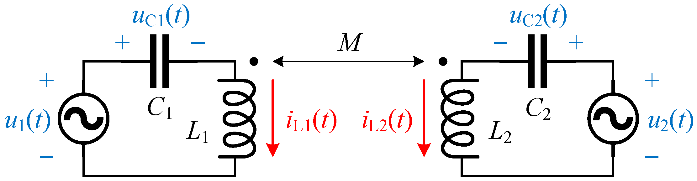
The frequency splitting phenomenon of coupled resonators is manifested as the gain peaks of the network appear at the so-called split frequencies, which are different from the resonant frequencies. The reason is that the eigenvalues of the coupled resonators drift with the increase in the coupling coefficient [20,21]. To show this more clearly, let us consider the coupled resonators shown in Figure 1, where L₁, C₁ and L₂, C₂ are the primary- and secondary-side inductance and capacitance, respectively; M is the mutual inductance; u₁ and u₂ are the ac excitation voltages; u_C1 and u_C2 are the resonant voltages; and i_L1 and i_L2 are the resonant currents.

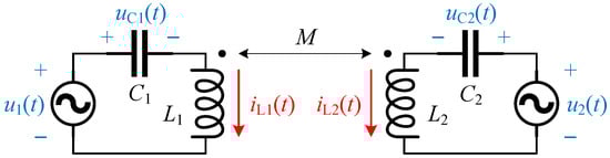
Figure 1. Magnetically coupled series resonators.

The instantaneous descriptor state-space model of the coupled resonators is given by

$$\begin{array}{c}\mathit{E}\frac{\mathrm{d}}{\mathrm{d}t}\left[\begin{array}{c}{i}_{\mathrm{L}1}\left(t\right)\\ i_{\mathrm{L}2}\left(t\right)\\ u_{\mathrm{C}1}\left(t\right)\\ u_{\mathrm{C}2}\left(t\right)\end{array}\right]=\mathit{A}\left[\begin{array}{c}{i}_{\mathrm{L}1}\left(t\right)\\ i_{\mathrm{L}2}\left(t\right)\\ u_{\mathrm{C}1}\left(t\right)\\ u_{\mathrm{C}2}\left(t\right)\end{array}\right]+\mathit{B}\left[\begin{array}{c}{u}_1\left(t\right)\\ u_2\left(t\right)\end{array}\right]\end{array}$$

(1)

where

$$\begin{array}{c}\left\{\begin{array}{l}\mathit{E}=\left[\begin{array}{cccc}{L}_1& M& 0& 0\\ M& L_2& 0& 0\\ 0& 0& C_1& 0\\ 0& 0& 0& C_2\end{array}\right]\\ \mathit{A}=\left[\begin{array}{cccc}0& 0& -1& 0\\ 0& 0& 0& -1\\ 1& 0& 0& 0\\ 0& 1& 0& 0\end{array}\right]\\ \mathit{B}=\left[\begin{array}{cc}1& 0\\ 0& 1\\ 0& 0\\ 0& 0\end{array}\right]\end{array}\right.\end{array}$$

(2)

In (1), i_L1 and i_L2 are taken as the output because they are directly coupled with the sources. The transfer functions from u₁ and u₂ to i_L1 and i_L2 deduced from (1) are expressed as

$$\begin{array}{c}\left[\begin{array}{cc}\frac{i_{\mathrm{L}1}\left(s\right)}{u_1\left(s\right)}& \frac{i_{\mathrm{L}1}\left(s\right)}{u_2\left(s\right)}\\ \frac{i_{\mathrm{L}2}\left(s\right)}{u_1\left(s\right)}& \frac{i_{\mathrm{L}2}\left(s\right)}{u_2\left(s\right)}\end{array}\right]=\frac{\left[\begin{array}{cc}{L}_{2}s\left(s^2+{\omega }_2^2\right)& -M{s}^3\\ -M{s}^3& L_{1}s\left(s^2+{\omega }_1^2\right)\end{array}\right]}{L_1{L}_2\left(1-k^2\right)\left(s^2+{\omega }_{\mathrm{o}}^2\right)\left(s^2+{\omega }_{\mathrm{e}}^2\right)}\end{array}$$

(3)

where k is the coupling coefficient:

$$\begin{array}{c}k=\frac{M}{\sqrt{L_1{L}_2}}\end{array}$$

(4)

ω₁ and ω₂ are the resonant frequencies:

$$\begin{array}{c}{\omega }_1=\frac{1}{\sqrt{L_1{C}_1}}, {\omega }_2=\frac{1}{\sqrt{L_2{C}_2}}\end{array}$$

(5)

ω_o and ω_e are the odd- and even-mode split frequencies:

$$\begin{array}{c}{\omega }_{\mathrm{o},\mathrm{e}}=\sqrt{\frac{\left({\omega }_1^2+{\omega }_2^2\right)\mp \sqrt{{\left({\omega }_1^2-{\omega }_2^2\right)}^2+4k^2{\omega }_1^2{\omega }_2^2}}{2\left(1-k^2\right)}}\end{array}$$

(6)

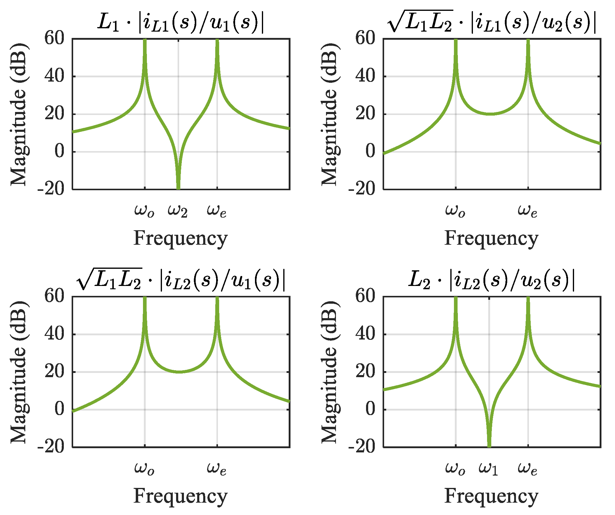
According to (3), the zeros of the coupled resonators locate at ±jω₁, ±jω₂, and 0, and the poles locate at ±jω_o and ±jω_e. Consequently, the gain valleys appear at ω₁ and ω₂, while the gain peaks appear at ω_o and ω_e, as shown by the bode diagrams in Figure 2.

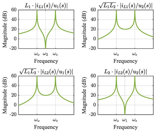
Figure 2. Bode diagrams of the coupled resonators.

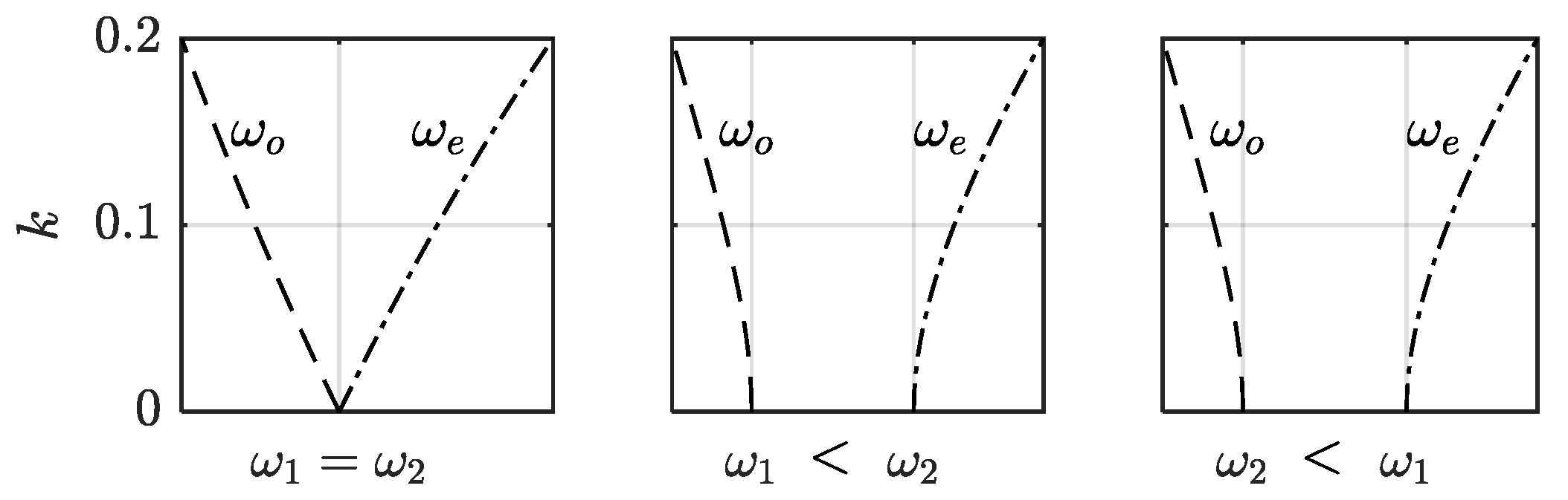
The split frequencies ω_o and ω_e are functions of the resonant frequencies ω₁ and ω₂ and the coupling coefficient k. When k increases, ω_o and ω_e gradually move away from ω₁ and ω₂, as shown in Figure 3.

Figure 3. Split frequencies as a function of coupling coefficient under three different cases: ω₁ = ω₂, ω₁ < ω₂, and ω₂ < ω₁.

3. Frequency Domain Analysis of the Dynamic Phasor Model

The state-space model in Section II takes the instantaneous voltages and currents at state variables. The model is intuitive in nature, but it does not reveal the magnitude and phase relationships between the ac excitation voltages and the resonant currents, which are of interest in dynamic control. This gap can be filled by the generalized state-space model or the dynamic phasor model when considering only the fundamental harmonic. In this section, we review the dynamic phasor model and provide the analysis of the frequency domain as the foundation of model reduction.

The dynamic phasor, X, of a signal, x, is a complex-valued number given by

$$\begin{array}{c}X\left(t\right)=\sqrt{2}{⟨x⟩}_1\left(t\right)=\frac{\sqrt{2}}{T_{\mathrm{s}}}{\int }_{t-T_{\mathrm{s}}}^{t}x\left(\tau \right){\mathrm{e}}^{-\mathrm{j}{\omega }_{\mathrm{s}}\tau }\mathrm{d}\tau \end{array}$$

(7)

where ω_s is the switching frequency and T_s the corresponding period. Usually, ω_s is set to the source frequency so that the dynamic phasor of the source is constant. The magnitude of X(t) corresponds to the amplitude of x, and the angle of X(t) is the phase of x. The derivative of X(t) with respect to time can be derived from (7) and expressed as

$$\begin{array}{c}\frac{\mathrm{d}X\left(t\right)}{\mathrm{d}t}=\sqrt{2}{⟨\frac{\mathrm{d}x}{\mathrm{d}t}⟩}_1\left(t\right)-\sqrt{2}j{\omega }_{\mathrm{s}}{⟨x⟩}_1\left(t\right)\end{array}$$

(8)

Let I_L1(t), I_L2(t), U_C1(t), U_C2(t), U₁(t), and U₂(t) represent the dynamic phasors of i_L1(t), i_L2(t), u_C1(t), u_C2(t), u₁(t), and u₂(t), respectively. By substituting the dynamic phasors and their derivatives into (1), it yields

$$\begin{array}{c}\mathit{E}\frac{\mathrm{d}}{\mathrm{d}t}\left[\begin{array}{c}{I}_{\mathrm{L}1}\left(t\right)\\ I_{\mathrm{L}2}\left(t\right)\\ U_{\mathrm{C}1}\left(t\right)\\ U_{\mathrm{C}2}\left(t\right)\end{array}\right]=\left(\mathit{A}-\mathrm{j}\omega \mathit{E}\right)\left[\begin{array}{c}{I}_{\mathrm{L}1}\left(t\right)\\ I_{\mathrm{L}2}\left(t\right)\\ U_{\mathrm{C}1}\left(t\right)\\ U_{\mathrm{C}2}\left(t\right)\end{array}\right]+\mathit{B}\left[\begin{array}{c}{U}_1\left(t\right)\\ U_2\left(t\right)\end{array}\right]\end{array}$$

(9)

Consequently, the transfer functions from U₁ and U₂ to I_L1 and I_L2 are

$$\begin{array}{c}\left[\begin{array}{cc}\frac{I_{\mathrm{L}1}\left(s\right)}{U_1\left(s\right)}& \frac{I_{\mathrm{L}1}\left(s\right)}{U_2\left(s\right)}\\ \frac{I_{\mathrm{L}2}\left(s\right)}{U_1\left(s\right)}& \frac{I_{\mathrm{L}2}\left(s\right)}{U_2\left(s\right)}\end{array}\right]=\frac{\left[\begin{array}{cc}{L}_2{s}^{\prime }\left({s^{\prime }}^2+{\omega }_2^2\right)& -M{s^{\prime }}^3\\ -M{s^{\prime }}^3& L_1{s}^{\prime }\left({s^{\prime }}^2+{\omega }_1^2\right)\end{array}\right]}{L_1{L}_2\left(1-k^2\right)\left({s^{\prime }}^2+{\omega }_{\mathrm{o}}^2\right)\left({s^{\prime }}^2+{\omega }_{\mathrm{e}}^2\right)}\end{array}$$

(10)

where

$$\begin{array}{c}{s}^{\prime }=s+j{\omega }_s\end{array}$$

(11)

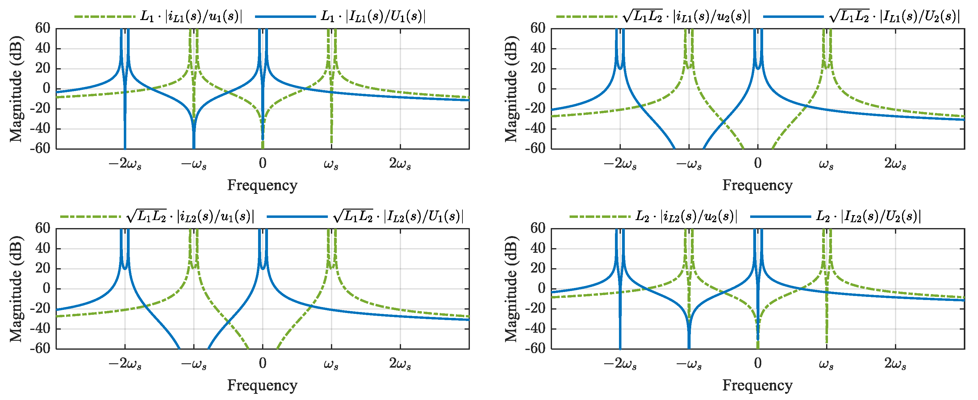
which means that the transfer functions between the dynamic phasors are obtained by shifting the transfer functions between the instantaneous signals in the frequency domain by −ω_s [22]. To illustrate this, Figure 4 compares the bode diagrams of (10) and (3). The bode diagrams are plotted along both positive and negative frequencies because (10) is complex-valued and is asymmetric in the frequency domain.

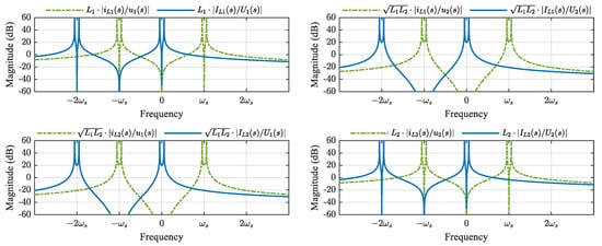
Figure 4. Bode diagrams of instantaneous model and dynamic phasor model when k = 0.1.

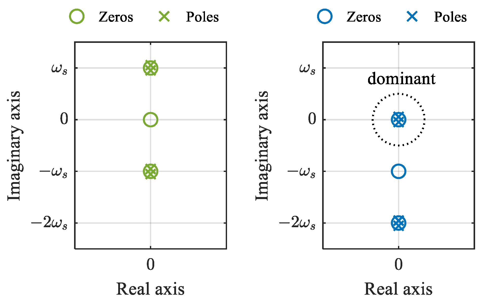
Furthermore, Figure 5 compares the zeros and poles of (3) and (10) on the complex plane. The zeros of (10) locate at ±jω₁ − jω_s, −jω_s ± jω₂, and −jω_s, and the poles locate at −jω_s ± jω_o and −jω_s ± jω_e, which are the translations of the zeros and poles of (3) along the imaginary axis, as indicated by (11). Considering that ω₁, ω₂, ω_o, ω_e, and ω_s are very close to each other, the dominant zeros of (10) are −jω_s + jω₁ and −jω_s + jω₂, and the dominant poles are −jω_s + jω_o and −jω_s + jω_e. On the complex plane, these dominant zeros and poles are within the circle whose radius is equal to the Nyquist frequency, i.e., ω_s/2, as shown in Figure 5. In a physical sense, the dominant zeros correspond to the beat frequencies, i.e.,

$$\begin{array}{c}\mathsf{\Delta }{\omega }_1={\omega }_{\mathrm{s}}-{\omega }_1, \mathsf{\Delta }{\omega }_2={\omega }_{\mathrm{s}}-{\omega }_2\end{array}$$

(12)

and the dominant poles correspond to the split beat frequencies, i.e.,

$$\begin{array}{c}\mathsf{\Delta }{\omega }_{\mathrm{o}}={\omega }_{\mathrm{s}}-{\omega }_{\mathrm{o}}, \mathsf{\Delta }{\omega }_{\mathrm{e}}={\omega }_{\mathrm{s}}-{\omega }_{\mathrm{e}}\end{array}$$

(13)

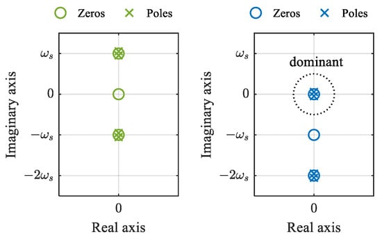
Figure 5. Zeros and poles of instantaneous model (left) and dynamic phasor model (right).

4. Order Reduction with Split Frequency Matching

The dynamic phasor model focuses on the signal magnitude and phase, which are low-frequency characteristics as compared with the switching frequency, ω_s. From this point of view, it is desired to find a reduced-order model that only contains dominant zeros and poles, i.e., −jω_s+jω₁, −jω_s+jω₂, −jω_s+jω_o, and −jω_s+jω_e. As there are two dominant poles and two dominant zeros, a reasonable formula for the reduced-order model is

$$\begin{array}{c}{\mathit{E}}_{\mathbf{r}}\frac{\mathrm{d}}{\mathrm{d}t}\left[\begin{array}{c}{I}_{\mathrm{L}1}\left(t\right)\\ I_{\mathrm{L}2}\left(t\right)\end{array}\right]={\mathit{A}}_{\mathbf{r}}\left[\begin{array}{c}{I}_{\mathrm{L}1}\left(t\right)\\ I_{\mathrm{L}2}\left(t\right)\end{array}\right]+{\mathit{B}}_{\mathbf{r}}\left[\begin{array}{c}{U}_1\left(t\right)\\ U_2\left(t\right)\end{array}\right]\end{array}$$

(14)

where E_r, A_r, and B_r are 2-by-2 coefficient matrices. For simplicity, one can let B_r be

$$\begin{array}{c}{\mathit{B}}_{\mathbf{r}}=\left[\begin{array}{cc}1& 0\\ 0& 1\end{array}\right]\end{array}$$

(15)

and then determine E_r and A_r by matching the steady-state gains and dominant zeros and poles of (14) with those of (9).

According to (9), the steady-state values of I_L1, I_L2, U₁, and U₂ satisfy

$$\begin{array}{c}\left[\begin{array}{c}{\overline{I}}_{\mathrm{L}1}\\ {\overline{I}}_{\mathrm{L}2}\end{array}\right]=-{\left(\mathit{A}-\mathrm{j}{\omega }_{\mathrm{s}}\mathit{E}\right)}^{-1}B\left[\begin{array}{c}{\overline{U}}_1\\ {\overline{U}}_2\end{array}\right]\end{array}$$

(16)

On the other hand, according to (14):

$$\begin{array}{c}\left[\begin{array}{c}{\overline{I}}_{\mathrm{L}1}\\ {\overline{I}}_{\mathrm{L}2}\end{array}\right]=-{\mathit{A}}_{\mathbf{r}}^{-1}{\mathit{B}}_{\mathbf{r}} \left[\begin{array}{c}{\overline{U}}_1\\ {\overline{U}}_2\end{array}\right]\end{array}$$

(17)

To match the results of (16) and (17), let

$$\begin{array}{c}-{\mathit{A}}_{\mathbf{r}}^{-1}{\mathit{B}}_{\mathbf{r}}=-{\left(\mathit{A}-\mathrm{j}{\omega }_{\mathrm{s}}\mathit{E}\right)}^{-1}B\end{array}$$

(18)

Then, it yields

$$\begin{array}{c}{\mathit{A}}_{\mathbf{r}}=\left[\begin{array}{cc}-\mathrm{j}\mathsf{\Delta }{\omega }_1{L}_{\mathsf{\omega }1}& -\mathrm{j}{\omega }_{\mathrm{s}}M\\ -\mathrm{j}{\omega }_{\mathrm{s}}M& -\mathrm{j}\mathsf{\Delta }{\omega }_2{L}_{\mathsf{\omega }2}\end{array}\right]\end{array}$$

(19)

where L_ω1 and L_ω2 are the equivalent inductances [14] given by

$$\begin{array}{c}{L}_{\mathsf{\omega }1}=\frac{{\omega }_{\mathrm{s}}+{\omega }_1}{{\omega }_{\mathrm{s}}}{L}_1, L_{\mathsf{\omega }2}=\frac{{\omega }_{\mathrm{s}}+{\omega }_2}{{\omega }_{\mathrm{s}}}{L}_2\end{array}$$

(20)

Let e₁₁, e₁₂, e₂₁, and e₂₂ be the undermined elements of E_r, i.e.,

$$\begin{array}{c}{\mathit{E}}_{\mathbf{r}}=\left[\begin{array}{cc}{e}_{11}& e_{12}\\ e_{21}& e_{22}\end{array}\right]\end{array}$$

(21)

With (21), the reduced transfer functions are deduced from (14) and expressed as

$$\begin{array}{c}\left[\begin{array}{cc}\frac{I_{\mathrm{L}1}\left(s\right)}{U_1\left(s\right)}& \frac{I_{\mathrm{L}1}\left(s\right)}{U_2\left(s\right)}\\ \frac{I_{\mathrm{L}2}\left(s\right)}{U_1\left(s\right)}& \frac{I_{\mathrm{L}2}\left(s\right)}{U_2\left(s\right)}\end{array}\right]=\frac{\left[\begin{array}{cc}{e}_{22}s+\mathrm{j}\mathsf{\Delta }{\omega }_2{L}_{\mathsf{\omega }2}& -e_{12}s-\mathrm{j}{\omega }_{\mathrm{s}}M\\ -e_{21}s-\mathrm{j}{\omega }_{\mathrm{s}}M& e_{11}s+\mathrm{j}\mathsf{\Delta }{\omega }_1{L}_{\mathsf{\omega }1}\end{array}\right]}{\mathsf{\Delta }\left(s\right)}\end{array}$$

(22)

where Δ(s) is the characteristic polynomial:

$$\begin{array}{c}\begin{array}{ll}\mathsf{\Delta }\left(s\right)=& \left(e_{11}s+\mathrm{j}\mathsf{\Delta }{\omega }_1{L}_{\mathsf{\omega }1}\right)\left(e_{22}s+\mathrm{j}\mathsf{\Delta }{\omega }_2{L}_{\mathsf{\omega }2}\right)\\ & -\left(e_{12}s+\mathrm{j}{\omega }_{\mathrm{s}}M\right)\left(e_{21}s+\mathrm{j}{\omega }_{\mathrm{s}}M\right)\end{array}\end{array}$$

(23)

To set the dominant zeros of (22) at −jω_s + jω₁ and −jω_s + jω₂, it is solved that

$$\begin{array}{c}{e}_{11}=L_{\mathsf{\omega }1}, e_{22}=L_{\mathsf{\omega }2}\end{array}$$

(24)

With (24), to set the dominant poles of (22) at −jω_s + jω_o and −jω_s + jω_e, it is solved that

$$\begin{array}{c}{e}_{12}=M_{\mathsf{\omega }}, e_{21}=M_{\mathsf{\omega }}^{*}\end{array}$$

(25)

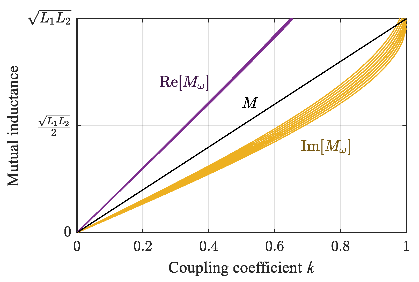
where M_ω and M_ω* are a pair of conjugate equivalent mutual inductances, which can be calculated using (26) and (27), derived from to the eigen equations of (9) and (22).

$$\begin{array}{c}{M}_{\mathsf{\omega }}+M_{\mathsf{\omega }}^{*}=\left(\frac{1}{k^2}·\frac{{\omega }_{\mathrm{s}}+{\omega }_1}{{\omega }_{\mathrm{s}}}·\frac{{\omega }_{\mathrm{s}}+{\omega }_2}{{\omega }_{\mathrm{s}}}·\frac{ \mathsf{\Delta }{\omega }_1+\mathsf{\Delta }{\omega }_2}{{\omega }_{\mathrm{s}}}+\frac{k^2-1}{k^2}·\frac{{\omega }_{\mathrm{s}}+{\omega }_{\mathrm{o}}}{{\omega }_{\mathrm{s}}}·\frac{{\omega }_{\mathrm{s}}+{\omega }_{\mathrm{e}}}{{\omega }_{\mathrm{s}}}·\frac{\mathsf{\Delta }{\omega }_{\mathrm{o}}+\mathsf{\Delta }{\omega }_{\mathrm{e}}}{{\omega }_{\mathrm{s}}}\right)M\end{array}$$

(26)

$$\begin{array}{c}{M}_{\mathsf{\omega }}{M}_{\mathsf{\omega }}^{*}=\left(\frac{1}{k^2}·\frac{{\omega }_{\mathrm{s}}+{\omega }_1}{{\omega }_{\mathrm{s}}}·\frac{{\omega }_{\mathrm{s}}+{\omega }_2}{{\omega }_{\mathrm{s}}}+\frac{k^2-1}{k^2}·\frac{{\omega }_{\mathrm{s}}+{\omega }_{\mathrm{o}}}{{\omega }_{\mathrm{s}}}·\frac{{\omega }_{\mathrm{s}}+{\omega }_{\mathrm{e}}}{{\omega }_{\mathrm{s}}}\right)M^2\end{array}$$

(27)

Figure 6 shows the real and imaginary parts of M_ω as functions of coupling coefficient k with ω₁ = ω_s ±5% and ω₂ = ω_s ±5%. It is found that Re[M_ω] and Im[M_ω] are almost linear with k in a wide range, like the mutual inductance M. The proportional factors of Re[M_ω] and Im[M_ω] to k depend on the relative error of ω₁ and ω₂ to ω_s but do not have large dispersions. Therefore, one can calculate M_ω and M_ω* using (28) and (29) instead of (26) and (27) for simplicity

$$\begin{array}{c}\underset{k\to 0}{\lim }\left(M_{\mathsf{\omega }}+M_{\mathsf{\omega }}^{*}\right)=\left[2+\frac{{\omega }_1+{\omega }_2}{2{\omega }_{\mathrm{s}}}+\frac{{\omega }_1{\omega }_2}{2\left({\omega }_1+{\omega }_2\right){\omega }_{\mathrm{s}}}-\frac{{\omega }_1^2{\omega }_2^2}{2\left({\omega }_1+{\omega }_2\right){\omega }_{\mathrm{s}}^3}\right]M\approx 3M\end{array}$$

(28)

$$\begin{array}{c}\underset{k\to 0}{\lim }{M}_{\mathsf{\omega }}{M}_{\mathsf{\omega }}^{*}=\left[1+\frac{{\omega }_1+{\omega }_2}{2{\omega }_{\mathrm{s}}}+\frac{{\omega }_1{\omega }_2}{2\left({\omega }_1+{\omega }_2\right){\omega }_{\mathrm{s}}}+\frac{{\omega }_1{\omega }_2}{2{\omega }_{\mathrm{s}}^2}\right]M^2\approx 2.75M^2\end{array}$$

(29)

and obtain

$$\begin{array}{c}{M}_{\mathsf{\omega }}\approx \left(\frac{3}{2}+\frac{1}{\sqrt{2}}\mathrm{j}\right)M, M_{\mathsf{\omega }}^{*}\approx \left(\frac{3}{2}-\frac{1}{\sqrt{2}}\mathrm{j}\right)M\end{array}$$

(30)

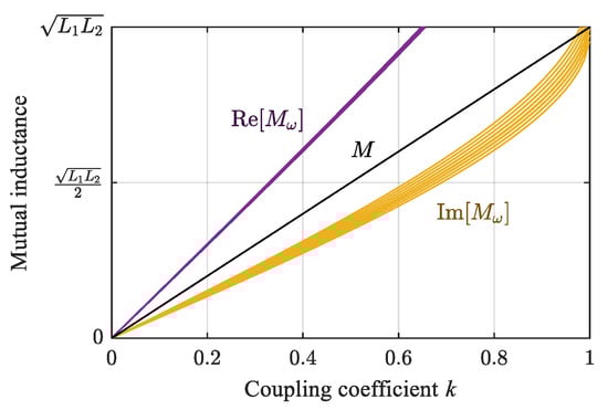
Figure 6. The real and imaginary parts of the equivalent mutual inductance, M_ω, as a function of coupling coefficient k.

With (24) and (25), E_r is rewritten as:

$$\begin{array}{c}{\mathit{E}}_{\mathbf{r}}=\left[\begin{array}{cc}{L}_{\mathsf{\omega }1}& M_{\mathsf{\omega }}\\ M_{\mathsf{\omega }}^{*}& L_{\mathsf{\omega }2}\end{array}\right]\end{array}$$

(31)

and the reduced transfer function is rewritten as

$$\begin{array}{c}\left[\begin{array}{cc}\frac{I_{\mathrm{L}1}\left(s\right)}{U_1\left(s\right)}& \frac{I_{\mathrm{L}1}\left(s\right)}{U_2\left(s\right)}\\ \frac{I_{\mathrm{L}2}\left(s\right)}{U_1\left(s\right)}& \frac{I_{\mathrm{L}2}\left(s\right)}{U_2\left(s\right)}\end{array}\right]=\frac{\left[\begin{array}{cc}{L}_{\mathsf{\omega }2}s+\mathrm{j}\mathsf{\Delta }{\omega }_2{L}_{\mathsf{\omega }2}& -M_{\mathsf{\omega }}s-\mathrm{j}{\omega }_{\mathrm{s}}M\\ -M_{\mathsf{\omega }}^{*}s-\mathrm{j}{\omega }_{\mathrm{s}}M& L_{\mathsf{\omega }1}s+\mathrm{j}\mathsf{\Delta }{\omega }_1{L}_{\mathsf{\omega }1}\end{array}\right]}{\left(L_{\mathsf{\omega }1}{L}_{\mathsf{\omega }2}-M_{\mathsf{\omega }}{M}_{\mathsf{\omega }}^{*}\right)\left(s+\mathrm{j}\mathsf{\Delta }{\omega }_{\mathrm{o}}\right)\left(s+\mathrm{j}\mathsf{\Delta }{\omega }_{\mathrm{e}}\right)}\end{array}$$

(32)

where

$$\begin{array}{c}\mathsf{\Delta }\left(s\right)=\left(L_{\mathsf{\omega }1}{L}_{\mathsf{\omega }2}-M_{\mathsf{\omega }}{M}_{\mathsf{\omega }}^{*}\right)\left(s+\mathrm{j}\mathsf{\Delta }{\omega }_{\mathrm{o}}\right)\left(s+\mathrm{j}\mathsf{\Delta }{\omega }_{\mathrm{e}}\right)\end{array}$$

(33)

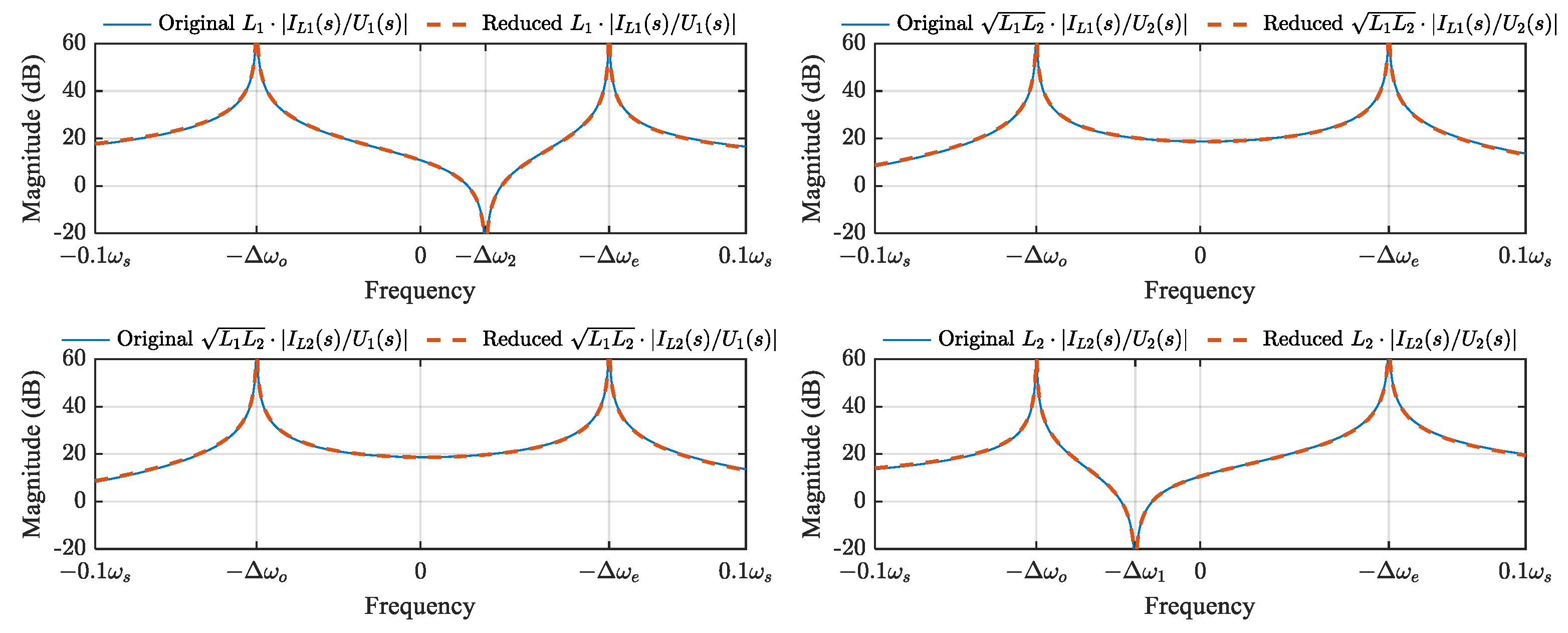
Figure 7 compares the bode diagrams of transfer function (32) derived from the reduced-order model to the bode diagrams of transfer function (10) derived from the original dynamic phasor model (10) within the frequency range from −0.1ω_s to 0.1ω_s. It is shown that the poles exactly locate at the split beat frequencies, and the two groups of transfer functions match with each other well, even when ω₂, ω₂, and ω_s are not identical. This means that the low-frequency characteristics of the original dynamic phasor model (9) can be precisely represented by the reduced-order model (14).

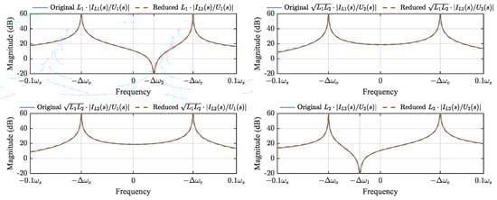
Figure 7. Bode diagrams of original and reduced dynamic phasor models when k = 0.1, ω₁ = 0.98ω_s, and ω₂ = 1.02ω_s.

5. Reduced Wpt System Model

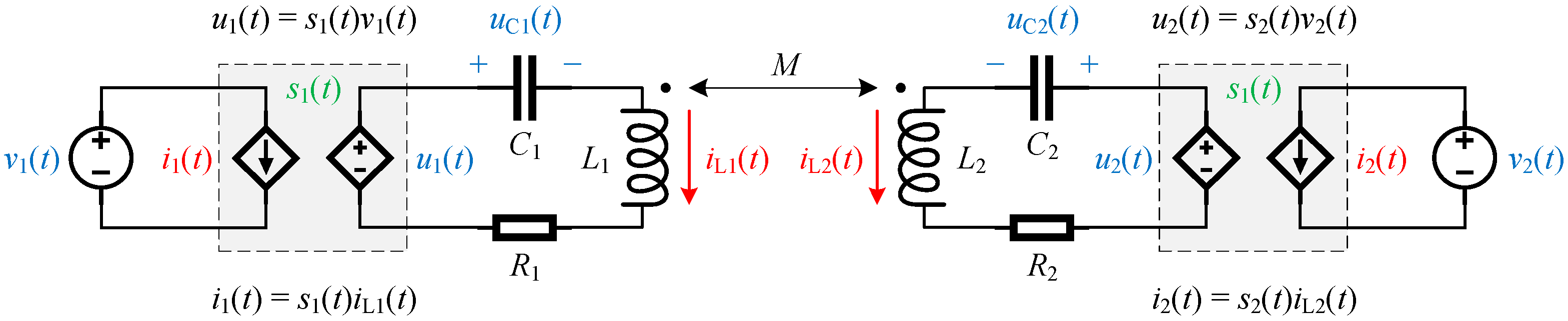
The coupled resonant network is essentially a linear system, and therefore, it is analyzed in the frequency domain in the above sections for order reduction. However, in a dc-to-dc WPT system, as shown in Figure 8, the most concerned relationships, e.g., the transfer functions between magnitudes used for power control, and the transfer functions between phases used for synchronization, can only be derived from a locally linearized small-signal model because the magnitudes and phases are nonlinear functions of dynamic phasors.

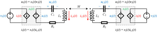
Figure 8. Dual-voltage-sourced WPT system based on magnetically coupled series resonators.

In Figure 8, the switching functions of the two converters are denoted by s₁ and s₂. For full-bridge converters, s₁ and s₂ may equal to 1, 0, and −1, depending on the switching control (for an active converter) or resonant current direction (for a diode rectifier). Consequently, the ac excitation voltages u₁ and u₂ are represented by the products of the switch functions and the dc side voltages v₁ and v₂ as

$$\begin{array}{c}\left\{\begin{array}{l}{u}_1\left(t\right)=s_1\left(t\right)v_1\left(t\right)\\ u_2\left(t\right)=s_2\left(t\right)v_2\left(t\right)\end{array}\right.\end{array}$$

(34)

and the dc side currents i₁ and i₂ are represented by the products of the switch functions and the resonant currents i_L1 and i_L2 as

$$\begin{array}{c}\left\{\begin{array}{l}{i}_1\left(t\right)=s_1\left(t\right)i_{\mathrm{L}1}\left(t\right)\\ i_2\left(t\right)=s_2\left(t\right)i_{\mathrm{L}2}\left(t\right)\end{array}\right.\end{array}$$

(35)

With the fundamental harmonic approximation, (33) and (34) can be rewritten as

$$\begin{array}{c}\left\{\begin{array}{l}{U}_1\left(t\right)=S_1\left(t\right)V_1\left(t\right)\\ U_2\left(t\right)=S_2\left(t\right)V_2\left(t\right)\end{array} \right.\end{array}$$

(36)

and

$$\begin{array}{c}\left\{\begin{array}{l}{I}_1\left(t\right)=\mathrm{R}\mathrm{e}\left[S_1^{*}\left(t\right)I_{\mathrm{L}1}\left(t\right)\right]\\ I_2\left(t\right)=\mathrm{R}\mathrm{e}\left[S_2^{*}\left(t\right)I_{\mathrm{L}2}\left(t\right)\right]\end{array}\right.\end{array}$$

(37)

where S₁ and S₂ are the dynamic phasors of s₁ and s₂, respectively, the superscript asterisk means to take the conjugate, and V₁, V₂, I₁, and I₂ are the moving averages of v₁, v₂, i₁, and i₂, respectively.

According to (35), the Jacobian matrix of ${\left(\mathrm{R}\mathrm{e}\left[U_1\right],\mathrm{R}\mathrm{e}\left[U_2\right],\mathrm{I}\mathrm{m}\left[U_1\right],\mathrm{I}\mathrm{m}\left[U_2\right]\right)}^T$ with respect to ${\left(V_1,\left|S_1\right|,\mathrm{\angle }{S}_1,V_2,\left|S_2\right|,\mathrm{\angle }{S}_2\right)}^T$ is

$$\begin{array}{c}{\mathit{J}}_{\mathbf{B}}=\left[\begin{array}{cccc}1& 0& 0& 0\\ 0& 0& 1& 0\\ 0& 1& 0& 0\\ 0& 0& 0& 1\end{array}\right]\left[\begin{array}{cc}\begin{array}{ccc}\frac{U_{1\mathrm{r}}}{V_1}& \frac{U_{1\mathrm{r}}}{\left|S_1\right|}& -U_{1\mathrm{i}}\\ \frac{U_{1\mathrm{i}}}{V_1}& \frac{U_{1\mathrm{i}}}{\left|S_1\right|}& U_{1\mathrm{r}}\end{array}& 0\\ 0& \begin{array}{ccc}\frac{U_{2\mathrm{r}}}{V_2}& \frac{U_{2\mathrm{r}}}{\left|S_2\right|}& -U_{2\mathrm{i}}\\ \frac{U_{2\mathrm{i}}}{V_2}& \frac{U_{2\mathrm{i}}}{\left|S_2\right|}& U_{2\mathrm{r}}\end{array}\end{array}\right]\end{array}$$

(38)

According to (36), the Jacobian matrix of ${\left(I_1,\left|I_{\mathrm{L}1}\right|,\mathrm{\angle }{I}_{\mathrm{L}1},I_2,\left|I_{\mathrm{L}2}\right|,\mathrm{\angle }{I}_{\mathrm{L}2}\right)}^T$ with respect to ${\left(\mathrm{R}\mathrm{e}\left[I_{\mathrm{L}1}\right],\mathrm{R}\mathrm{e}\left[I_{\mathrm{L}2}\right],\mathrm{I}\mathrm{m}\left[I_{\mathrm{L}1}\right],\mathrm{I}\mathrm{m}\left[I_{\mathrm{L}2}\right]\right)}^T$ is

$$\begin{array}{c}{\mathit{J}}_{\mathbf{C}}=\left[\begin{array}{cc}\begin{array}{cc}{S}_{1\mathrm{r}}& S_{1\mathrm{i}}\\ \frac{I_{\mathrm{L}1\mathrm{r}}}{\left|I_{\mathrm{L}1}\right|}& \frac{I_{\mathrm{L}1\mathrm{i}}}{\left|I_{\mathrm{L}1}\right|}\\ -\frac{I_{\mathrm{L}1\mathrm{i}}}{{\left|I_{\mathrm{L}1}\right|}^2}& \frac{I_{\mathrm{L}1\mathrm{r}}}{{\left|I_{\mathrm{L}1}\right|}^2}\end{array}& 0\\ 0& \begin{array}{cc}{S}_{2\mathrm{r}}& S_{2\mathrm{i}}\\ \frac{I_{\mathrm{L}2\mathrm{r}}}{\left|I_{\mathrm{L}2}\right|}& \frac{I_{\mathrm{L}2\mathrm{i}}}{\left|I_{\mathrm{L}2}\right|}\\ -\frac{I_{\mathrm{L}2\mathrm{i}}}{{\left|I_{\mathrm{L}2}\right|}^2}& \frac{I_{\mathrm{L}2\mathrm{r}}}{{\left|I_{\mathrm{L}2}\right|}^2}\end{array}\end{array}\right]\left[\begin{array}{cccc}1& 0& 0& 0\\ 0& 0& 1& 0\\ 0& 1& 0& 0\\ 0& 0& 0& 1\end{array}\right]\end{array}$$

(39)

and the Jacobian matrix of ${\left(I_1,\left|I_{\mathrm{L}1}\right|,\mathrm{\angle }{I}_{\mathrm{L}1},I_2,\left|I_{\mathrm{L}2}\right|,\mathrm{\angle }{I}_{\mathrm{L}2}\right)}^T$ with respect to ${\left(V_1,\left|S_1\right|,\mathrm{\angle }{S}_1,V_2,\left|S_2\right|,\mathrm{\angle }{S}_2\right)}^T$ is

$$\begin{array}{c}{\mathit{J}}_{\mathbf{D}}=\left[\begin{array}{cc}\begin{array}{ccc}0& \frac{I_1}{\left|S_1\right|}& \mathrm{I}\mathrm{m}\left[S_1^{*}{I}_{\mathrm{L}1}\right]\\ 0& 0& 0\\ 0& 0& 0\end{array}& 0\\ 0& \begin{array}{ccc}0& \frac{I_2}{\left|S_2\right|}& \mathrm{I}\mathrm{m}\left[S_2^{*}{I}_{\mathrm{L}2}\right]\\ 0& 0& 0\\ 0& 0& 0\end{array}\end{array}\right]\end{array}$$

(40)

Meanwhile, the reduced-order model (14) is rewritten in an expanded real-valued form as

$$\begin{array}{c}\begin{array}{cc}f\left({\mathit{E}}_{\mathbf{r}}\right)\frac{\mathrm{d}}{\mathrm{d}t}\left[\begin{array}{c}\begin{array}{c}\mathrm{R}\mathrm{e}\left[I_{\mathrm{L}1}\left(t\right)\right]\\ \mathrm{R}\mathrm{e}\left[I_{\mathrm{L}1}\left(t\right)\right]\end{array}\\ \begin{array}{c}\mathrm{I}\mathrm{m}\left[I_{\mathrm{L}2}\left(t\right)\right]\\ \mathrm{I}\mathrm{m}\left[I_{\mathrm{L}2}\left(t\right)\right]\end{array}\end{array}\right]=& f\left({\mathit{A}}_{\mathbf{r}}-{\mathit{R}}_{\mathbf{r}}\right)\left[\begin{array}{c}\begin{array}{c}\mathrm{R}\mathrm{e}\left[I_{\mathrm{L}1}\left(t\right)\right]\\ \mathrm{R}\mathrm{e}\left[I_{\mathrm{L}1}\left(t\right)\right]\end{array}\\ \begin{array}{c}\mathrm{I}\mathrm{m}\left[I_{\mathrm{L}2}\left(t\right)\right]\\ \mathrm{I}\mathrm{m}\left[I_{\mathrm{L}2}\left(t\right)\right]\end{array}\end{array}\right]\\ & +f\left({\mathit{B}}_{\mathbf{r}}\right)\left[\begin{array}{c}\begin{array}{c}\mathrm{R}\mathrm{e}\left[U_1\left(t\right)\right]\\ \mathrm{R}\mathrm{e}\left[U_2\left(t\right)\right]\end{array}\\ \begin{array}{c}\mathrm{I}\mathrm{m}\left[U_1\left(t\right)\right]\\ \mathrm{I}\mathrm{m}\left[U_2\left(t\right)\right]\end{array}\end{array}\right]\end{array}\end{array}$$

(41)

where R_r is the equivalent series resistance (ESR) matrix introduced by R₁ and R₂:

$$\begin{array}{c}{\mathit{R}}_{\mathbf{r}}=\left[\begin{array}{cc}{R}_1& 0\\ 0& R_2\end{array}\right]\end{array}$$

(42)

and f maps a complex matrix Z to an expanded real-valued matrix as

$$\begin{array}{c}f\left(\mathit{Z}\right)=\left[\begin{array}{cc}\mathrm{R}\mathrm{e}\left[\mathit{Z}\right]& -\mathrm{I}\mathrm{m}\left[\mathit{Z}\right]\\ \mathrm{I}\mathrm{m}\left[\mathit{Z}\right]& \mathrm{R}\mathrm{e}\left[\mathit{Z}\right]\end{array}\right]\end{array}$$

(43)

By substituting (37)–(39) into (40), the small-signal model of the WPT system is obtained:

$$\begin{array}{c}\left\{\begin{array}{l}\begin{array}{cc}f\left({\mathit{E}}_{\mathbf{r}}\right)\frac{\mathrm{d}}{\mathrm{d}t}\left[\begin{array}{c}\begin{array}{c}\mathrm{R}\mathrm{e}\left[{\widehat{I}}_{\mathrm{L}1}\left(t\right)\right]\\ \mathrm{R}\mathrm{e}\left[{\widehat{I}}_{\mathrm{L}1}\left(t\right)\right]\end{array}\\ \begin{array}{c}\mathrm{I}\mathrm{m}\left[{\widehat{I}}_{\mathrm{L}2}\left(t\right)\right]\\ \mathrm{I}\mathrm{m}\left[{\widehat{I}}_{\mathrm{L}2}\left(t\right)\right]\end{array}\end{array}\right]=& f\left({\mathit{A}}_{\mathbf{r}}-{\mathit{R}}_{\mathbf{r}}\right)\left[\begin{array}{c}\begin{array}{c}\mathrm{R}\mathrm{e}\left[{\widehat{I}}_{\mathrm{L}1}\left(t\right)\right]\\ \mathrm{R}\mathrm{e}\left[{\widehat{I}}_{\mathrm{L}1}\left(t\right)\right]\end{array}\\ \begin{array}{c}\mathrm{I}\mathrm{m}\left[{\widehat{I}}_{\mathrm{L}2}\left(t\right)\right]\\ \mathrm{I}\mathrm{m}\left[{\widehat{I}}_{\mathrm{L}2}\left(t\right)\right]\end{array}\end{array}\right]\\ & +f\left({\mathit{B}}_{\mathbf{r}}\right){\mathit{J}}_{\mathbf{B}}\left[\begin{array}{c}\begin{array}{c}{\widehat{V}}_1\left(t\right)\\ \left|{\widehat{S}}_1\right|\left(t\right)\\ \angle {\widehat{S}}_1\left(t\right)\end{array}\\ \begin{array}{c}{\widehat{V}}_2\left(t\right)\\ \left|{\widehat{S}}_2\right|\left(t\right)\\ \angle {\widehat{S}}_2\left(t\right)\end{array}\end{array}\right]\end{array}\\ \left[\begin{array}{c}\begin{array}{c}{\widehat{I}}_1\left(t\right)\\ \left|{\widehat{I}}_{\mathrm{L}1}\right|\left(t\right)\\ \angle {\widehat{I}}_{\mathrm{L}1}\left(t\right)\end{array}\\ \begin{array}{c}{\widehat{I}}_2\left(t\right)\\ \left|{\widehat{I}}_{\mathrm{L}2}\right|\left(t\right)\\ \angle {\widehat{I}}_{\mathrm{L}2}\left(t\right)\end{array}\end{array}\right]={\mathit{J}}_{\mathbf{C}}\left[\begin{array}{c}\begin{array}{c}\mathrm{R}\mathrm{e}\left[{\widehat{I}}_{\mathrm{L}1}\left(t\right)\right]\\ \mathrm{R}\mathrm{e}\left[{\widehat{I}}_{\mathrm{L}1}\left(t\right)\right]\end{array}\\ \begin{array}{c}\mathrm{I}\mathrm{m}\left[{\widehat{I}}_{\mathrm{L}2}\left(t\right)\right]\\ \mathrm{I}\mathrm{m}\left[{\widehat{I}}_{\mathrm{L}2}\left(t\right)\right]\end{array}\end{array}\right]+{\mathit{J}}_{\mathbf{D}}\left[\begin{array}{c}\begin{array}{c}{\widehat{V}}_1\left(t\right)\\ \left|{\widehat{S}}_1\right|\left(t\right)\\ \angle {\widehat{S}}_1\left(t\right)\end{array}\\ \begin{array}{c}{\widehat{V}}_2\left(t\right)\\ \left|{\widehat{S}}_2\right|\left(t\right)\\ \angle {\widehat{S}}_2\left(t\right)\end{array}\end{array}\right]\end{array}\right.\end{array}$$

(44)

Equation (43) is a 4th-order real-valued small-signal model with 6 input signals and 6 output signals, including both magnitudes and phases of the control signals, dc voltages, and resonant currents.

Based on (43), the 6-by-6 small-signal transfer function matrix from the input vector ${\left(V_1, \left|S_1\right|,\angle S_1,V_2,\left|S_2\right|,\angle S_2\right)}^T$ to the output vector ${\left(I_1, \left|I_{\mathrm{L}1}\right|,\angle I_{\mathrm{L}1},I_2,\left|I_{\mathrm{L}2}\right|,\angle I_{\mathrm{L}2}\right)}^T$, which may contain all the concerned information of the WPT system, is derived from (43) and expressed as

$$\begin{array}{c}\begin{array}{l}\left[\begin{array}{cc}\begin{array}{ccc}\frac{{\widehat{I}}_1\left(s\right)}{{\widehat{V}}_1\left(s\right)}& \frac{{\widehat{I}}_1\left(s\right)}{\left|{\widehat{S}}_1\right|\left(s\right)}& \frac{{\widehat{I}}_1\left(s\right)}{\angle {\widehat{S}}_1\left(s\right)}\\ \frac{\left|{\widehat{I}}_{\mathrm{L}1}\right|\left(s\right)}{{\widehat{V}}_1\left(s\right)}& \frac{\left|{\widehat{I}}_{\mathrm{L}1}\right|\left(s\right)}{\left|{\widehat{S}}_1\right|\left(s\right)}& \frac{\left|{\widehat{I}}_{\mathrm{L}1}\right|\left(s\right)}{\angle {\widehat{S}}_1\left(s\right)}\\ \frac{\angle {\widehat{I}}_{\mathrm{L}1}\left(s\right)}{{\widehat{V}}_1\left(s\right)}& \frac{\angle {\widehat{I}}_{\mathrm{L}1}\left(s\right)}{\left|{\widehat{S}}_1\right|\left(s\right)}& \frac{\angle {\widehat{I}}_{\mathrm{L}1}\left(s\right)}{\angle {\widehat{S}}_1\left(s\right)}\end{array}& \begin{array}{ccc}\frac{{\widehat{I}}_1\left(s\right)}{{\widehat{V}}_2\left(s\right)}& \frac{{\widehat{I}}_1\left(s\right)}{\left|{\widehat{S}}_2\right|\left(s\right)}& \frac{{\widehat{I}}_1\left(s\right)}{\angle {\widehat{S}}_2\left(s\right)}\\ \frac{\left|{\widehat{I}}_{\mathrm{L}1}\right|\left(s\right)}{{\widehat{V}}_2\left(s\right)}& \frac{\left|{\widehat{I}}_{\mathrm{L}1}\right|\left(s\right)}{\left|{\widehat{S}}_2\right|\left(s\right)}& \frac{\left|{\widehat{I}}_{\mathrm{L}1}\right|\left(s\right)}{\angle {\widehat{S}}_2\left(s\right)}\\ \frac{\angle {\widehat{I}}_{\mathrm{L}1}\left(s\right)}{{\widehat{V}}_2\left(s\right)}& \frac{\angle {\widehat{I}}_{\mathrm{L}1}\left(s\right)}{\left|{\widehat{S}}_2\right|\left(s\right)}& \frac{\angle {\widehat{I}}_{\mathrm{L}1}\left(s\right)}{\angle {\widehat{S}}_2\left(s\right)}\end{array}\\ \begin{array}{ccc}\frac{{\widehat{I}}_2\left(s\right)}{{\widehat{V}}_1\left(s\right)}& \frac{{\widehat{I}}_2\left(s\right)}{\left|{\widehat{S}}_1\right|\left(s\right)}& \frac{{\widehat{I}}_2\left(s\right)}{\angle {\widehat{S}}_1\left(s\right)}\\ \frac{\left|{\widehat{I}}_{\mathrm{L}2}\right|\left(s\right)}{{\widehat{V}}_1\left(s\right)}& \frac{\left|{\widehat{I}}_{\mathrm{L}2}\right|\left(s\right)}{\left|{\widehat{S}}_1\right|\left(s\right)}& \frac{\left|{\widehat{I}}_{\mathrm{L}2}\right|\left(s\right)}{\angle {\widehat{S}}_1\left(s\right)}\\ \frac{\angle {\widehat{I}}_{\mathrm{L}2}\left(s\right)}{{\widehat{V}}_1\left(s\right)}& \frac{\angle {\widehat{I}}_{\mathrm{L}2}\left(s\right)}{\left|{\widehat{S}}_1\right|\left(s\right)}& \frac{\angle {\widehat{I}}_{\mathrm{L}2}\left(s\right)}{\angle {\widehat{S}}_1\left(s\right)}\end{array}& \begin{array}{ccc}\frac{{\widehat{I}}_2\left(s\right)}{{\widehat{V}}_2\left(s\right)}& \frac{{\widehat{I}}_2\left(s\right)}{\left|{\widehat{S}}_2\right|\left(s\right)}& \frac{{\widehat{I}}_1\left(s\right)}{\angle {\widehat{S}}_2\left(s\right)}\\ \frac{\left|{\widehat{I}}_{\mathrm{L}2}\right|\left(s\right)}{{\widehat{V}}_2\left(s\right)}& \frac{\left|{\widehat{I}}_{\mathrm{L}2}\right|\left(s\right)}{\left|{\widehat{S}}_2\right|\left(s\right)}& \frac{\left|{\widehat{I}}_{\mathrm{L}2}\right|\left(s\right)}{\angle {\widehat{S}}_2\left(s\right)}\\ \frac{\angle {\widehat{I}}_{\mathrm{L}2}\left(s\right)}{{\widehat{V}}_2\left(s\right)}& \frac{\angle {\widehat{I}}_{\mathrm{L}2}\left(s\right)}{\left|{\widehat{S}}_2\right|\left(s\right)}& \frac{\angle {\widehat{I}}_{\mathrm{L}2}\left(s\right)}{\angle {\widehat{S}}_2\left(s\right)}\end{array}\end{array}\right]\\ ={\mathit{J}}_{\mathbf{C}}{\left[sf\left({\mathit{E}}_{\mathbf{r}}\right)-f\left({\mathit{A}}_{\mathbf{r}}-{\mathit{R}}_{\mathbf{r}}\right)\right]}^{-1}f\left({\mathit{B}}_{\mathbf{r}}\right){\mathit{J}}_{\mathbf{B}}+{\mathit{J}}_{\mathbf{D}}\end{array}\end{array}$$

(45)

6. Experimental Verification

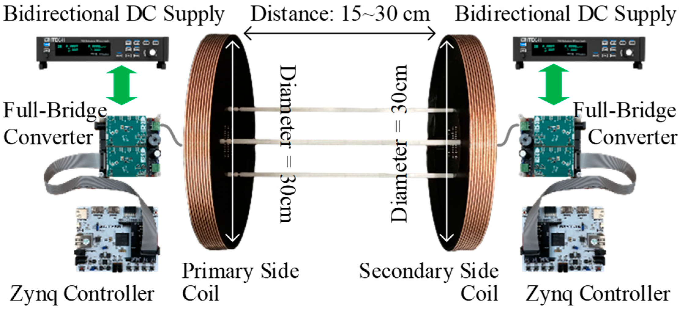
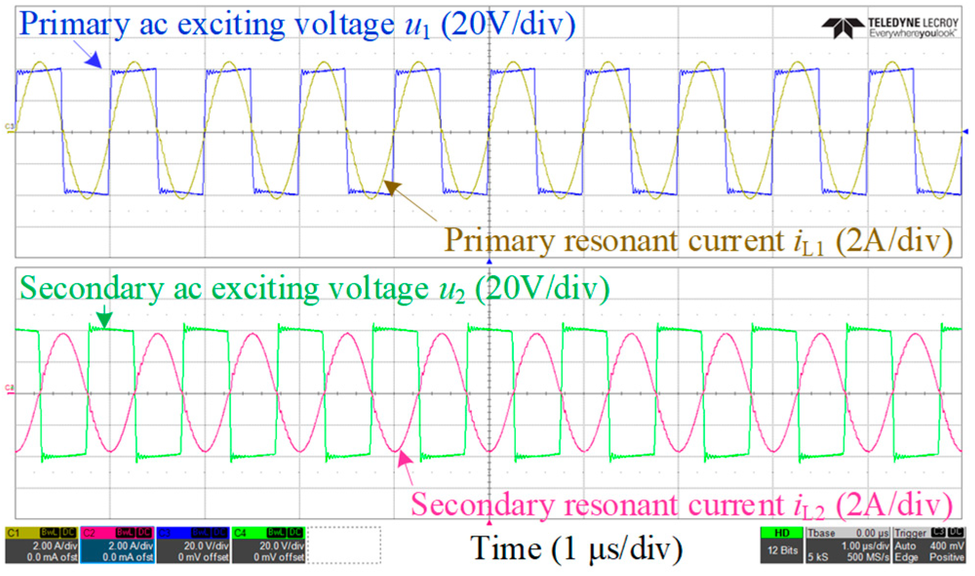
The accuracy of the proposed reduced-order model is verified in this section by the low-power experimental system shown in Figure 9. The system consisted of a pair of coupled resonators made of AWG 46 Litz wires, high-Q ceramic capacitors, and two gallium-nitride full-bridge converters controlled by Zynq development boards. To focus on the dynamics of the WPT stage, the converters were directly fed by bidirectional dc supplies so that the characteristics predicted by the reduced-order state-space model (14) and the transfer functions in (44) could be directly measured and verified. The nominal operating parameters of the system are listed in Table 1, and the steady-state operating waveforms are shown in Figure 10. The transferred power was 100 W and the dc-to-dc efficiency was 93.5%. Thanks to the high-efficiency GaN devices and zero-voltage switching (ZVS) operation [23], the losses on the converters were insignificant and most of the system power loss came from the ESR of the coils. For model verification, the representative dynamic characteristics of the system, including both large-signal step responses under ON–OFF control, and the small-signal bode diagrams at steady states, were measured and compared to the model predictions under different test conditions, as listed in Table 2.

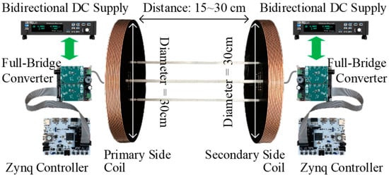
Figure 9. Experimental WPT system.

Table 1. Nominal operating parameters.

Symbol	Quantity	Value
L1,2	Resonant inductances	63.3 μH
C1,2	Resonant capacitances	400 pF
fr1,2	Resonant frequencies	1 MHz
fs	Switching frequency	1 MHz
R1,2	ESRs	~1 Ω
Q1,2	Quality factors	400
k	Coupling coefficient	0.1
D	Power transfer distance	15 cm
V1,2	DC supply voltages	40 V

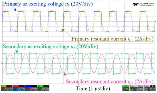
Figure 10. Steady-state operating waveforms with nominal operating parameters.

Table 2. Test conditions.

Operating Condition	Coupling Coefficient	Switching Frequency
Tuned resonance w/strong coupling	k = 0.1	fs = 1 MHz
Detuned resonance w/strong coupling	k = 0.1	fs = 1.02 MHz
Tuned resonance w/week coupling	k = 0.03	fs = 1 MHz

6.1. Large-Signal Characteristics

A simple control method for low-power WPT applications is the ON–OFF keying method introduced in [24]. The average power is controlled by periodically operating the primary-side converter between ON and OFF periods, e.g., for a full-bridge converter, switching s₁ between 1 and −1 during ON periods and keeping s₁ = 0 during OFF periods.

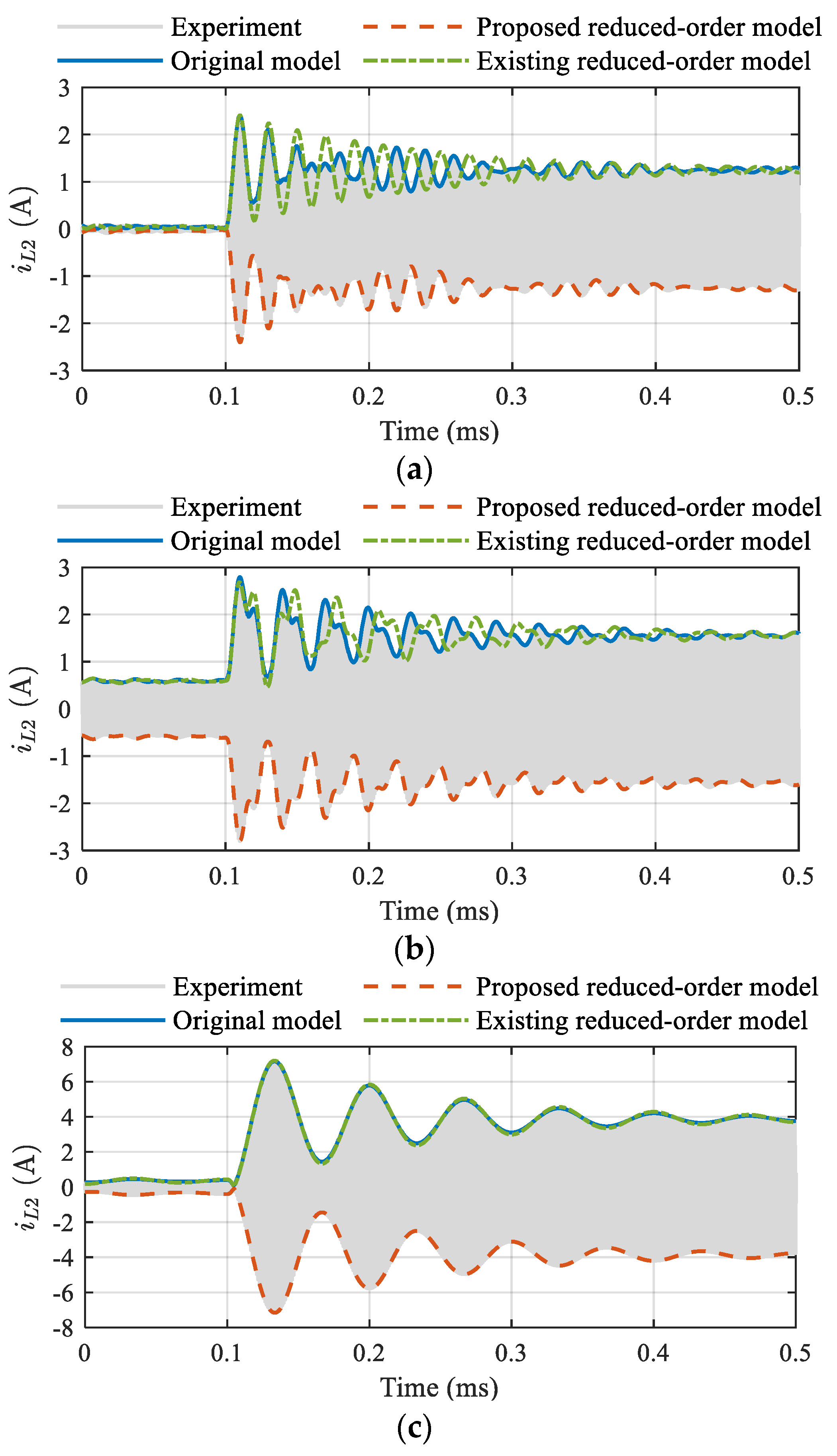
Figure 11 shows the waveforms of secondary-side resonant current i_L2 at the beginning of an ON period. The magnitude of i_L2, i.e., |I_L2|, oscillated quickly when the coupling was strong and oscillated slowly when the coupling was weak. The reason is that the oscillations depend on the split beat frequencies Δω_o and Δω_e, and the split beat frequencies depend on the coupling coefficient. When the system was slightly detuned, the oscillation mode became more complicated because the beat frequencies Δω₁ and Δω₂ were no longer zero. Under all tested operation conditions, the proposed reduced-order model (14) and the original dynamic phasor model matched the experimental results (envelopes) well. In contrast, the existing reduced-order model [14] was accurate, only with weak coupling, and had accumulated errors when the coupling was relatively strong.

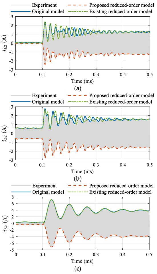
Figure 11. Time-domain responses of secondary-side resonant current when turning on the primary-side converter when the system is (a) tuned with strong coupling, (b) detuned with strong coupling, and (c) with weak coupling.

6.2. Small-Signal Characteristics

Synchronizing the secondary-side converter of a WPT system with its primary-side converter is crucial for stable power transfer. For an active secondary-side converter, the synchronization requires a phase-locked loop that adjusts the phase of the converter drive signal according to the phase of the measured resonant current [25]. The stability of the synchronization depends on the closed-loop phase dynamics, which involve the small-signal transfer function from the drive signal phase angle, i.e., $\angle S_2$, to the resonant current phase angle, i.e., $\angle I_{\mathrm{L}2}$.

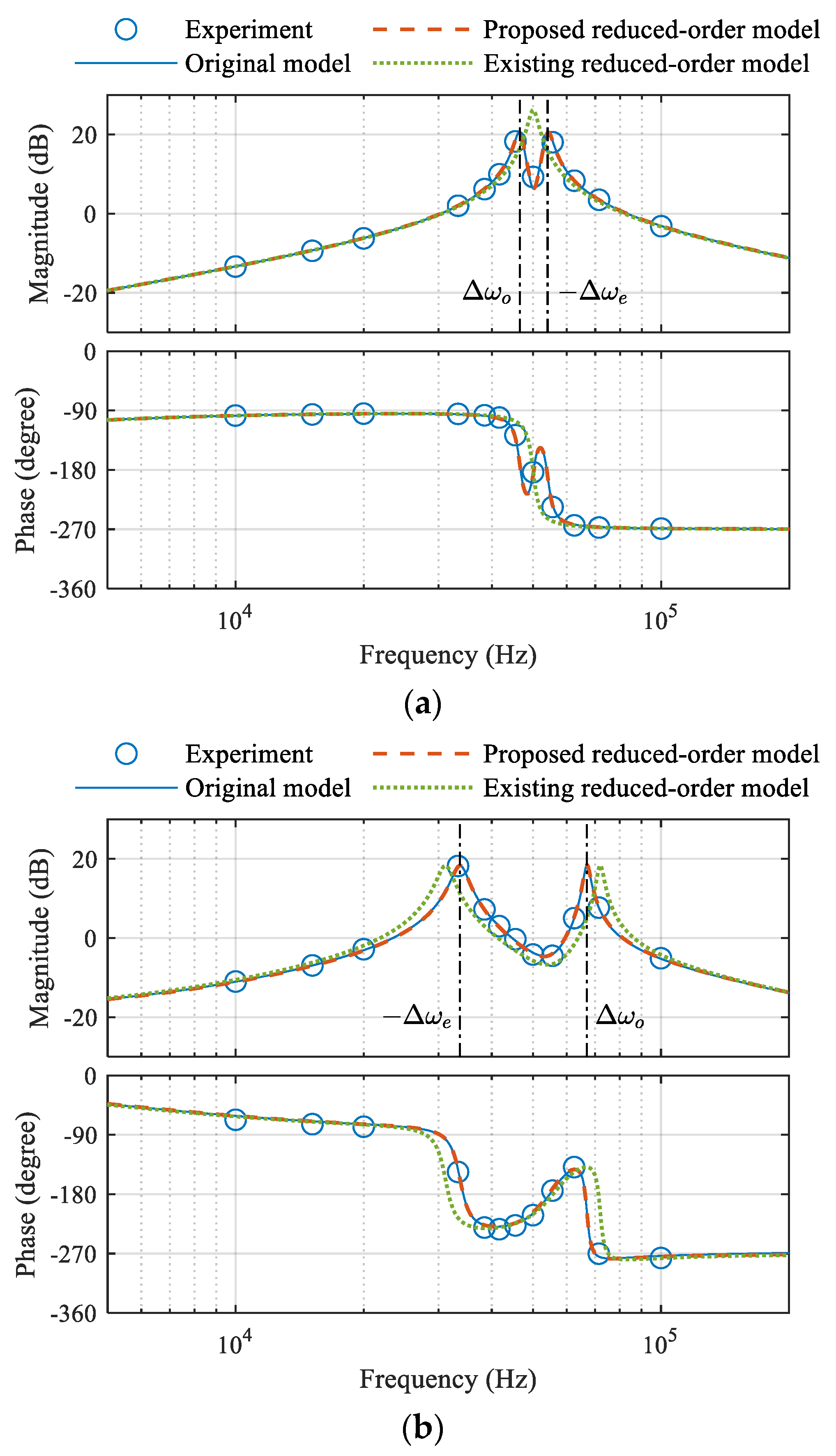
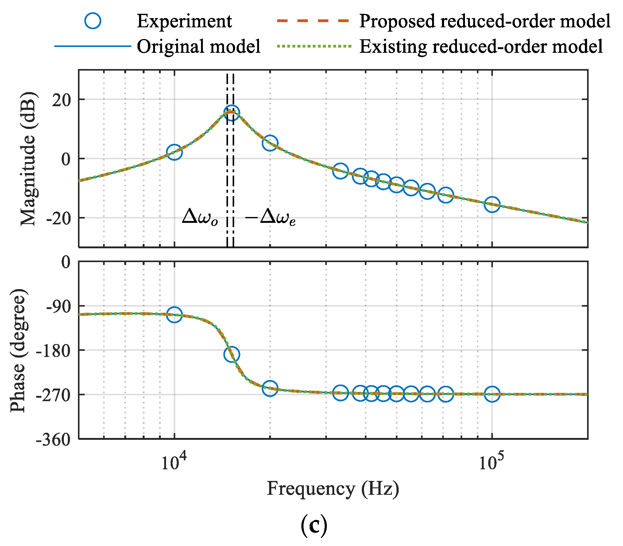
In the experiment, to obtain the small-signal bode diagram of the transfer function $\angle I_{\mathrm{L}2}\left(\mathrm{s}\right)/\angle S_2\left(\mathrm{s}\right)$, a low-frequency (10~100 kHz) phase perturbation signal of 7.2° magnitude (corresponding to 20 ns) was injected into the steady-state $\angle S_2$ using a variable time-delay unit, and the responded $\angle I_{\mathrm{L}2}$ was measured by a high-bandwidth current transformer (CST4835), a zero-crossing detector (LMH7220), and a digital phase detector on the Zynq board. Then, the measured time-domain data of $\angle S_2$ and $\angle I_{\mathrm{L}2}$ were processed with discrete Fourier transform to obtain $\angle I_{\mathrm{L}2}\left(\mathrm{s}\right)/\angle S_2\left(\mathrm{s}\right)$ at a particular perturbation frequency. Figure 12 shows the small-signal bode diagrams at the steady states of different operating conditions. When the coupling was strong, the gain curve had two peaks that corresponded to the split beat frequencies Δω_o and −Δω_e, as shown in Figure 12a,b. When the coupling was weak, the two gain peaks merged into one, as shown in Figure 12c. Under all tested operation conditions, both the proposed reduced-order model and the original dynamic phasor model accurately predicted the small-signal characteristics. However, the existing reduced-order model failed to predict the two gain peaks under the tuned and strong coupling condition, and had a bit peak frequency error under the detuned condition.

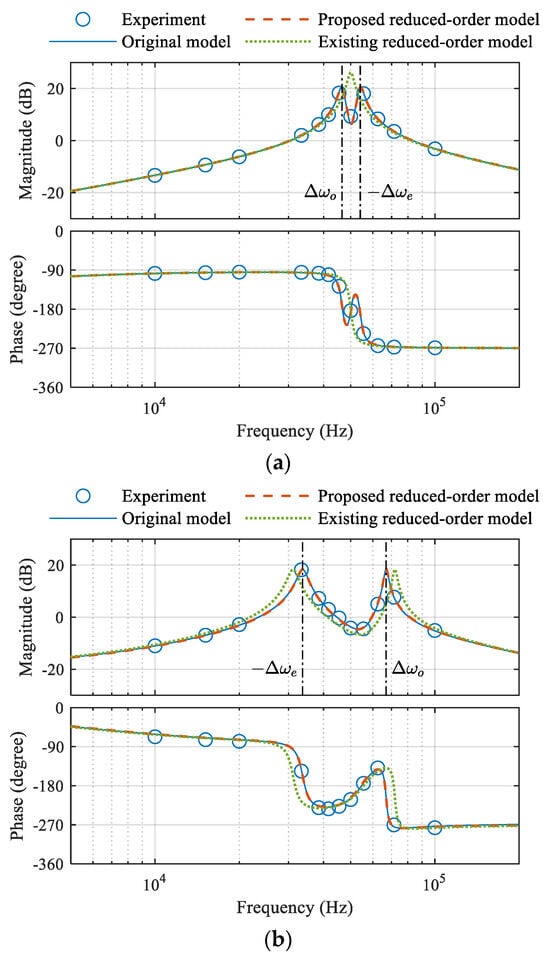
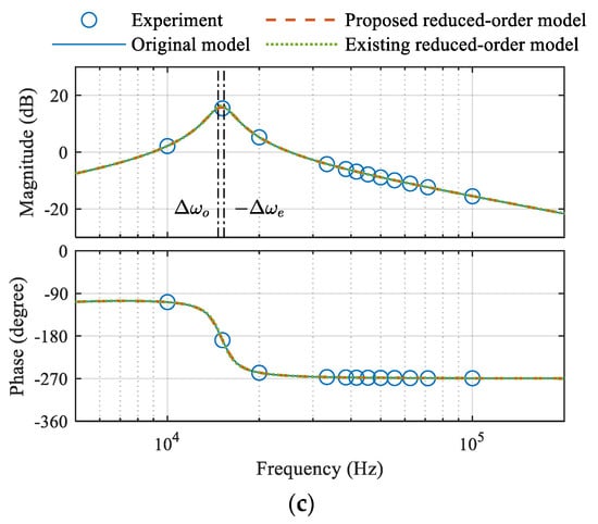
Figure 12. Bode diagram of $\angle I_{\mathrm{L}2}\left(\mathrm{s}\right)/\angle S_2\left(\mathrm{s}\right)$ when the system is (a) tuned with strong coupling, (b) detuned with strong coupling, and (c) with weak coupling.

7. Conclusions

This paper improved the accuracy of the reduced-order dynamic phasor model of WPT systems with strongly coupled resonators, where the split frequencies are dominant in the dynamic characteristics. Compared with the existing reduced-order model, the major change is a pair of conjugate equivalent mutual inductance derived from split beat frequency matching. Due to the equivalent mutual inductances, the asymmetry characteristics of the full-order dynamic phasor model in positive and negative frequency domains are completely preserved. The proposed model maintains a simple formula and low computational cost, while significantly improving accuracy under strong coupling conditions, as revealed by the large-signal and small-signal experimental tests. The model is useful for the dynamic analysis and control design of WPT systems with either weak or strong coupling, such as short-distance wireless EV charging.

References

- Buja, G.; Choi, S.Y.; Rim, C.T. Modern Advances in Wireless Power Transfer Systems for Roadway Powered Electric Vehicles. IEEE Trans. Ind. Electron. 2016, 63, 6533–6545. [Google Scholar] [CrossRef]
- Hui, S.Y. Planar Wireless Charging Technology for Portable Electronic Products and Qi. Proc. IEEE 2013, 101, 1290–1301. [Google Scholar] [CrossRef]
- Zhang, Z.; Pang, H.; Georgiadis, A.; Cecati, C. Wireless power transfer—An overview. IEEE Trans. Ind. Electron. 2019, 66, 1044–1058. [Google Scholar] [CrossRef]
- Zhong, W.; Hui, S.R. Charging Time Control of Wireless Power Transfer Systems Without Using Mutual Coupling Information and Wireless Communication System. IEEE Trans. Ind. Electron. 2017, 64, 228–235. [Google Scholar] [CrossRef]
- Huang, Z.; Wong, S.-C.; Tse, C.K. Control design for optimizing efficiency in inductive power transfer systems. IEEE Trans. Power Electron. 2018, 33, 4523–4534. [Google Scholar] [CrossRef]
- Jiang, Y.; Wang, L.; Wang, Y.; Wu, M.; Zeng, Z.; Liu, Y.; Sun, J. Phase-locked loop combined with chained trigger mode used for impedance matching in wireless high power transfer. IEEE Trans. Power Electron. 2020, 35, 4272–4285. [Google Scholar] [CrossRef]
- Hu, A.P. Modeling a contactless power supply using GSSA method. In Proceedings of the 2009 IEEE International Conference on Industrial Technology, Churchill, VIC, Australia, 10–13 February 2009; pp. 1–6. [Google Scholar]
- Hao, H.; Covic, G.A.; Boys, J.T. An approximate dynamic model of LCL-T-based inductive power transfer power supplies. IEEE Trans. Power Electron. 2014, 29, 5554–5567. [Google Scholar] [CrossRef]
- Sanders, S.R.; Noworolski, J.M.; Liu, X.Z.; Verghese, G.C. Generalized averaging method for power conversion circuits. IEEE Trans. Power Electron. 1991, 6, 251–259. [Google Scholar] [CrossRef]
- Yang, E.X.; Lee, F.C.; Jovanovic, M.M. Small-signal modeling of series and parallel resonant converters. In Proceedings of the IEEE Applied Power Electronics Conference and Exposition (APEC), Boston, MA, USA, 23–27 February 1992; pp. 785–792. [Google Scholar]
- Rim, C.T.; Cho, G.H. Phasor transformation and its application to the DC/AC analyses of frequency phase-controlled series resonant converters (SRC). IEEE Trans. Power Electron. 1990, 5, 201–211. [Google Scholar] [CrossRef]
- Lee, S.; Choi, B.; Rim, C.T. Dynamics characterization of the inductive power transfer system for online electric vehicles by Laplace phasor transform. IEEE Trans. Power Electron. 2013, 28, 5902–5909. [Google Scholar] [CrossRef]
- Li, H.; Wang, K.; Huang, L.; Chen, W.; Yang, X. Dynamic Modeling Based on Coupled Modes for Wireless Power Transfer Systems. IEEE Trans. Power Electron. 2015, 30, 6245–6253. [Google Scholar] [CrossRef]
- Li, H.; Fang, J.; Tang, Y. Dynamic phasor-based reduced-order models of wireless power transfer systems. IEEE Trans. Power Electron. 2019, 34, 11361–11370. [Google Scholar] [CrossRef]
- Tang, J.; Dong, S.; Cui, C.; Zhang, Q. Sampled-Data Modeling for Wireless Power Transfer Systems. IEEE Trans. Power Electron. 2020, 35, 3173–3182. [Google Scholar] [CrossRef]
- Chen, F.; Padilla, A.; Young, P.C.; Garnier, H. Data-Driven Modeling of Wireless Power Transfer Systems With Slowly Time-Varying Parameters. IEEE Trans. Power Electron. 2020, 35, 12442–12456. [Google Scholar] [CrossRef]
- Chen, F.; Young, P.C.; Garnier, H.; Deng, Q.; Kazimierczuk, M.K. Data-Driven Modeling of Wireless Power Transfer Systems With Multiple Transmitters. IEEE Trans. Power Electron. 2020, 35, 11363–11379. [Google Scholar] [CrossRef]
- Gawronski, W.; Juang, J.-N. Model reduction in limited time and frequency intervals. Int. J. Syst. Sci. 1990, 21, 349–376. [Google Scholar] [CrossRef]
- SAE J2954_202010; Wireless Power Transfer for Light-Duty Plug-In and Electric Vehicles and Alignment Methodology. SAE International: Warrendale, PA, USA, 2016.
- Niu, W.Q.; Chu, J.X.; Gu, W.; Shen, A.D. Exact Analysis of Frequency Splitting Phenomena of Contactless Power Transfer Systems. IEEE Trans. Circuits Syst. I-Regul. Pap. 2013, 60, 1670–1677. (In English) [Google Scholar] [CrossRef]
- Haus, H.A.; Huang, W. Coupled-mode theory. Proc. IEEE 1991, 79, 1505–1518. [Google Scholar] [CrossRef]
- Tan, T.; Chen, K.; Lin, Q.; Jiang, Y.; Yuan, L.; Zhao, Z. Impedance Shaping Control Strategy for Wireless Power Transfer System Based on Dynamic Small-Signal Analysis. IEEE Trans. Circuits Syst. I 2021, 68, 1354–1365. [Google Scholar] [CrossRef]
- Li, H.; Wang, K.; Fang, J.; Tang, Y. Pulse density modulated ZVS full-bridge converters for wireless power transfer systems. IEEE Trans. Power Electron. 2019, 34, 369–377. [Google Scholar] [CrossRef]
- Zhong, W.; Hui, S.Y.R. Maximum energy efficiency operation of series-series resonant wireless power transfer systems using on-off keying modulation. IEEE Trans. Power Electron. 2018, 33, 3595–3603. [Google Scholar] [CrossRef]
- Jia, S.; Chen, C.; Liu, P.; Duan, S. A digital phase synchronization method for bidirectional inductive power transfer. IEEE Trans. Ind. Electron. 2020, 67, 6450–6460. [Google Scholar] [CrossRef]
Disclaimer/Publisher’s Note: The statements, opinions and data contained in all publications are solely those of the individual author(s) and contributor(s) and not of MDPI and/or the editor(s). MDPI and/or the editor(s) disclaim responsibility for any injury to people or property resulting from any ideas, methods, instructions or products referred to in the content. |
© 2024 by the authors. Licensee MDPI, Basel, Switzerland. This article is an open access article distributed under the terms and conditions of the Creative Commons Attribution (CC BY) license (https://creativecommons.org/licenses/by/4.0/).