Article

Wearable Loops for Dynamic Monitoring of Joint Flexion: A Machine Learning Approach

1
ElectroScience Laboratory, Department of Electrical and Computer Engineering, The Ohio State University, Columbus, OH 43212, USA
2
Department of Electrical and Electronic Engineering, Bangladesh University of Engineering and Technology, Dhaka 1205, Bangladesh
*
Author to whom correspondence should be addressed.
Electronics 2024, 13(12), 2245; https://doi.org/10.3390/electronics13122245
Submission received: 19 April 2024 / Revised: 30 May 2024 / Accepted: 5 June 2024 / Published: 7 June 2024
(This article belongs to the Special Issue Wearable Electronics for Noninvasive Sensing)

Abstract

:
We present a machine learning driven system to monitor joint flexion angles during dynamic motion, using a wearable loop-based sensor. Our approach uses wearable loops to collect transmission coefficient data and an Artificial Neural Network (ANN) with fine-tuned parameters to increase accuracy of the measured angles. We train and validate the ANN for sagittal plane flexion of a leg phantom emulating slow motion, walking, brisk walking, and jogging. We fabricate the loops on conductive threads and evaluate the effect of fabric drift via measurements in the absence and presence of fabric. In the absence of fabric, our model produced a root mean square error (RMSE) of 5.90°, 6.11°, 5.90°, and 5.44° during slow motion, walking, brisk walking, and jogging. The presence of fabric degraded the RMSE to 8.97°, 7.21°, 9.41°, and 7.79°, respectively. Without the proposed ANN method, errors exceeded 35.07° for all scenarios. Proof-of-concept results on three human subjects further validate this performance. Our approach empowers feasibility of wearable loop sensors for motion capture in dynamic, real-world environments. Increasing speed of motion and the presence of fabric degrade sensor performance due to added noise. Nevertheless, the proposed framework is generalizable and can be expanded upon in the future to improve upon the reported angular resolution.

1. Introduction

Motion capture in real-world environments (i.e., outside the lab) is becoming increasingly important and useful. Examples include monitoring of Parkinson’s disease [1] and recovery after Anterior Cruciate Ligament Reconstruction (ACLR) [2], gaming [3], e-sports [4], and human–computer interaction applications [5,6]. However, state-of-the-art motion capture technologies lack seamlessness and/or accuracy, particularly in real-world environments.
Referring to Table 1, marker-based or markerless cameras require a contrived environment to work in [7,8,9], while changes to these environments can have detrimental effects on the accuracy of the results [10]. Inertial Measurement Units (IMUs) may be portable/wearable [11] but are bulky and accumulate errors over the course of time (known as integration drift) [12]. Time-of-flight sensors require line-of-sight and are hindered by the slightest obstruction in between the path of two antennas [13,14]. Retractable string sensors can be obstructive and depend highly on position on the limb, so if a patient does not place their device in the correct place, then accuracy will be compromised [15]. Bending sensors can be obtrusive and restrict natural motion, while their accuracy degrades with the number of flexes [16,17,18]. A Magnetic, Angular Rate, and Gravity (MARG) sensor system may be rather small but still depends on integration, which could lead to greater errors in a real-world environment and requires a rather complicated calibration technique [19,20,21]. Additionally, while a magnetometer–accelerometer system may be accurate in a lab-controlled setting, its bulkiness and specific requirements for calibration may affect its performance in the real world [22].
To overcome these limitations, we recently reported an alternative solution based on electrically small loop antennas (hereafter referred to as loops) that are placed above and below the joint, respectively, hence misaligning as the joint moves, Figure 1 [23,24]. In brief, the loop above the joint transmits electromagnetic (EM) energy in the inductive regime, while the loop below the joint receives energy and generates voltage based on Faraday’s law. A mapping process is then pursued to map the transmission coefficient (|S21|) values into joint angles. Note that the setup of Figure 1 is suitable for joint flexion monitoring and that a second receiving loop can be added to monitor joint rotation as well [23].
Our previous research has shown the efficacy of using loops to monitor joint angles in simulations as well as in tissue-emulating phantoms [23]. However, experimental validation was oversimplified for the sake of proving the concept, having the following three major limitations: (1) The loops were embedded in a 3D-printed fixture to maintain their circular shape, and they were placed tangentially upon the body, but not conformally. They were also fabricated on rigid copper wire. In real-world settings though, the loops are envisioned to be fabricated on flexible conductive threads (e-threads) and placed conformally upon the body. (2) Our previous studies only considered static motion, i.e., the phantom limb was fixed at a given angle, and transmission coefficient values were subsequently measured. However, motion happens in a dynamic way, with angles changing as a function of time. This dynamic motion is expected to increase the noise of the measurements (instrument noise as well as motional electromotive force), hence degrading the accuracy of the retrieved angles. Such errors have been unaccounted for to date. (3) The loops were tested stand-alone without being embedded in any type of fabric. In real-world settings though, the loops will be embedded in some form of clothing (e.g., leggings), meaning that fabric drift (stretching, pulling, deformation, etc.) will alter the loop geometry and relative position of the loops during motion. Indeed, fabric drift has been previously identified as potentially detrimental in textile sensor performance [25], while past efforts to reduce this error have once again considered static data [26] and not dynamic motion.
In this work, we take a major step forward to overcome the loop limitations outlined above. We focus on the flexion-monitoring setup of Figure 1, though the findings and approach are generalizable to other configurations as well. We perform studies on tissue-emulating phantoms using (1) e-thread-based loops that are conformal to the limb, (2) dynamic motion that also accounts for the factor of speed, and (3) fabric to embed the loops in (while also performing studies in the absence of fabric to better understand its effects). Our results confirm that, in the presence of these three real-world considerations, our previous mapping of transmission coefficient values into angles is highly erroneous. Our results also confirm similar performance for human subject testing as compared to phantom testing. As such, a machine-learning approach is brought forward to post-process the data and reduce errors. Due to its powerful ability to detect nuances and anomalies in data, machine learning can allow for more accurate predictions and models that can be generalized to a variety of different settings [27,28]. In this context, this work expands upon our previously reported loop-based sensors for motion capture and integrates an Artificial Neural Network (ANN) with fine-tuned parameters to increase accuracy of the measured angles in the motion, presence of fabric, and flexible e-thread implementation of the loops. In Section 2, we explain our data collection process and machine learning framework. In Section 3, we document the results of our approach in terms of sensical error metrics and figures. In Section 4, we explain our results, plans for future work, and apply our approach to a sample of human subjects.

2. Materials and Methods

2.1. Overview of the Approach

The proposed approach used to predict dynamic flexion angle measurements from transmission coefficient (|S21|) measurements is summarized in Figure 2. First, experimental |S21| data are collected using a network analyzer along with “gold-standard” angles obtained via a depth-sensing camera. We note that the sensor loops act as electrically small loop antennas, implying that the receiving loop is significantly less sensitive to the electrical field signal as compared to the magnetic field signal received from the transmitting loop. That is, we can consider the two loops as magnetically coupled, and electrical noise is of no concern. Noise in the environment would only be relevant when a metal plate (or equivalent) approaches the sensor. This aspect will be explored in the future. A multi-step data preprocessing method is then employed to denoise and establish clear relationships between inputs and targets. This data preprocessing block is discussed in detail in Section 2.3.1. Next, the data are split into three datasets—for hyperparameter-tuning, cross-validation, and graphical evaluation. Here, an ANN is the chosen model, because future work may explore data from multiple sets of loops resulting in much higher dimensionality, and it is well known that ANNs are best suited for high-dimensional data.
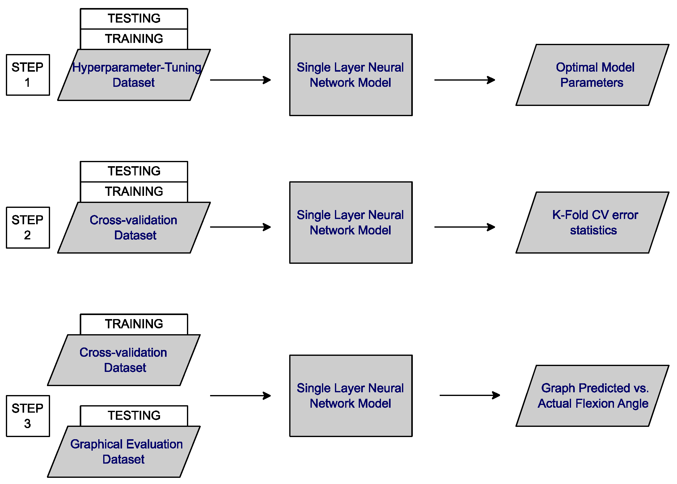
Then, we apply three machine learning steps. These are visualized in Figure 3. First, we use the hyperparameter-tuning dataset to grid search for the optimal hyperparameters for the neural network model (Figure 3, step 1). This model, with these hyperparameters, is used for the remaining experiments. Then, we use the cross-validation dataset to perform a 5-Fold Cross Validation (CV)—evaluating model performance and testing for overfitting (Figure 3, step 2). We want to ensure that this model is accurate for all data, not just a specific subset of the data. Then, we train the model on the entire cross-validation dataset and test on the graphical evaluation dataset (Figure 3, step 3). We use these predictions to graph the model’s predicted vs. actual angle values.

2.2. Data Acquisition System and Methods

2.2.1. Experimental Setup

To mimic flexion of the knee joint, a Styrofoam leg phantom was used. Without loss of generality, this particular phantom allows for sagittal plane flexion between 0.46° and 122.79°, per the definition in Figure 4a. Figure 4a shows the definition of the sagittal flexion angle, by identifying the location of the utilized measurement markers. Note that since loops are operated in the inductive regime, their operation is insensitive to the presence or absence of tissue [23]. The phantom was made of two Styrofoam cylinders with radius 4 cm and length 38 cm. A 3D-printed joint was attached to both cylinders so that they could move analogously to a human joint. The cylinders were subsequently glued onto the 3D-printed fixture in order to prevent rotation which would obfuscate measurements. On the center of the joint and the ends of both cylinders, small strips of reflective tape were placed so that “gold-standard” angles could be detected using camera-based methods.
We created two sets of loops, namely, “sleeveless” and “sleeved”, all with an 8 cm radius, made resonant at 34 MHz using a series capacitor (102 pF), as seen in Figure 4. They were all fabricated using automated embroidery of Liberator-40 e-threads and fed through an SMA connector. The “sleeveless” loops (Figure 4a) entailed two separate loops, each embroidered into a non-stretchy fabric square. The two squares were separate, i.e., not attached to each other, to eliminate the effect of fabric presence pulling upon the joint. On the phantom, these squares were taped 10 cm apart across the joint so that one square is on each Styrofoam cylinder. Next, sleeves were created with embedded loops to simulate a real-world “sleeved” design (Figure 4b). We used a polyester–spandex fabric to allow for the loops to expand and contract as they would in a real-world setting. Both loops were embroidered onto the fabric, with the ends of the loops 10 cm apart.

2.2.2. Data Collection

We used a Keysight PNA-L Network Analyzer to measure transmission coefficient (|S21|) values between the loops at 34 MHz and an Intel RealSense 2 Depth Perception Camera to determine the “gold-standard” angle that the phantom was at. This camera setup has been validated in our lab against a goniometer, demonstrating a root mean squared error (RMSE) of 0.32°. A goniometer setup could instead have been selected to collect the “gold standard” angles. For example, this has been the case in our previous work with static data collection [24]. Based on this past experience, we purposely select a camera-based setup in this study to (a) facilitate collection of dynamic data, (b) empower automated syncing with the network analyzer measurements, and (c) reduce human error. An in-house Python-based tool was developed to dynamically collect and synchronize the network analyzer and camera measurements. We note that the camera had a frame rate of 30 frames/s, whereas the network analyzer was sampling data at 60 points/s. To effectively compare the two sets of data, the flexion angle data were interpolated with respect to the time values of the |S21| data. Specifically, after data collection, we have two streams of data, from each of the collection equipment (camera for flexion angle, network analyzer for |S21|). The network analyzer collected at a speed of 60 frames per second, and the camera collected at 30 frames per second. It was necessary to convert these two data streams into one time domain. So, we use linear interpolation to obtain a new stream of angle values with points at the same time steps as the |S21| values.
To collect data, we manually flexed the phantom at a fixed speed for 15 s. This duration was chosen to ensure consistency of the measurements, given the manual nature of flexing. We purposedly avoided a motorized setup to eliminate noise associated with sources that would not be present in a realistic human setup. Trials were pursued at four (4) different speeds, namely, slow, walking, brisk walking, and jogging. The speeds of the trials were calculated based on the average rotations per minute of each of the movements [29,30], converted to number of flexions per 15 s. Table 2 shows each speed with the number of flexions performed in a 15 s time period. For each speed, we collected trials with both the “sleeveless” and the “sleeved” sets of loops. For every loop and speed combination, we collected eight (8) 15 s trials. This was a suitable number of trials such that big data could be achieved; the neural network model would have enough information to make optimal predictions. More trials would have made the training process slow and unable to perform detailed analysis.

2.3. Machine Learning Framework

2.3.1. Data Preprocessing

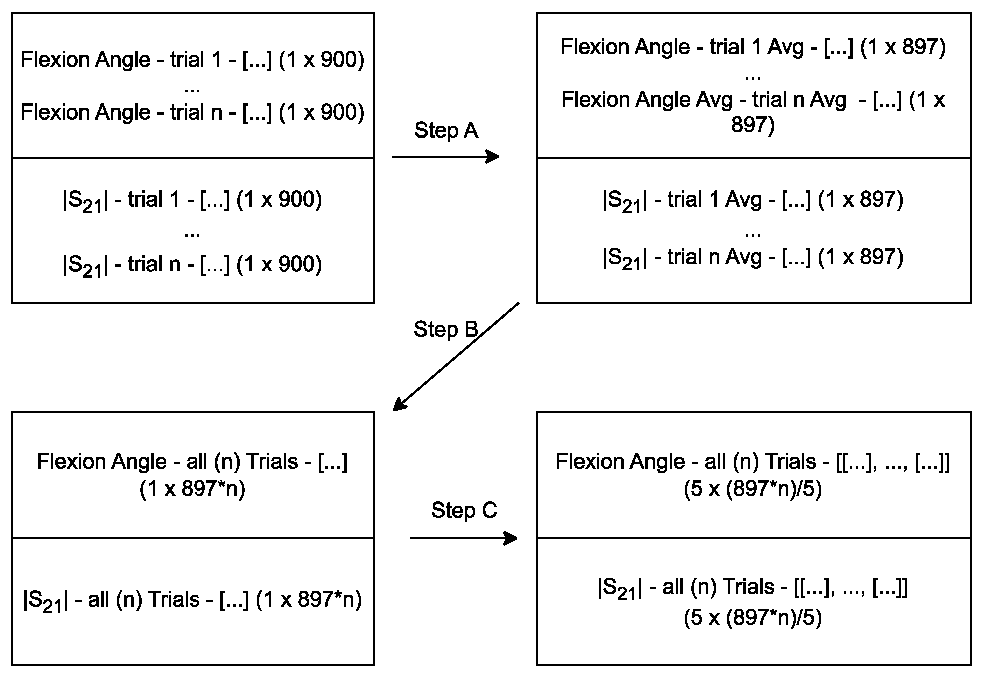
Let us consider n as the number of trials we record and 900 as the number of (|S21|, flexion angle) pairs we record per trial. First, a moving average with window size of 5 was applied to the |S21| coefficient and flexion angle vectors for each trial. This was carried out to reduce noise in the |S21| data so that the ANN can make more accurate predictions of flexion angle, based only on input |S21| data from wearable loops on the phantom arm (Step A in Figure 5). This window size was chosen after comparing the training error for the same basic model and several different window sizes. Specifically, during our training process, we tested input vectors where a moving average was both applied and not applied. Performance was maximized with a moving average (window size = 5). This is true, as the moving average lessens the impacts of noisy points that are significantly different from other points around them with respect to time. Then, after applying the moving average, we have 896 pairs per trial. Keeping all data in order with respect to time, we create two (1 row × n × 896 column) vectors, each representing all |S21| and all flexion angle data (Step B in Figure 5). Next, we create two reshaped matrices (also representing all |S21| data, all flexion angle data) from the previous (1 × n × 896 column) vectors. Every five consecutive elements in each previous vector become an element in the new corresponding matrix. Then, each matrix is sized (5 × (896 × n)/5) (Step C in Figure 5).
We assert that the delta in between vector elements will be relevant for the model to generalize and make accurate predictions on all speeds of trials. Also, as there may be noise in the |S21| readings, having a multi-element vector output will allow us to filter out inaccurate and spurious elements. We choose to size the vector as 5 because we require several elements to observe outliers, but a larger vector would cause inefficiencies in training the neural network.
Specifically, n = 8 × 8 = 64 (8 motion tasks and 8 trials per task). A |S21| coefficient signal matrix (rows: ⌊8 tasks [sleeved and sleeveless for each of the four speeds described in Table 2] × 8 trials per task × 896 timestamps [one per measurement]/5 |S21| elements⌋ = 11,468; columns: 5 |S21| elements) and a corresponding flexion angle matrix (rows: ⌊8 tasks [sleeved and sleeveless for each of the four speeds described in Table 2] × 8 trials per task × 896 timestamps [one per measurement]/5 flexion angle elements⌋ = 11,468; columns: 5 flexion angle elements) result as the processed data. In other words, each |S21| flexion angle element from each of the trials recorded is included in each of the matrices. Every 5 consecutive elements are included in their own row. These matrices are separated to form the datasets defined below and utilized as training/testing data in Figure 3.
For example, Figure 6 shows (|S21|, flexion angle) data points as recorded with respect to time, for sleeveless (a) and sleeved (b) trials. Then, vectors from (c) are in the matrices described above. We utilize three sets of data throughout this work. First, we select one trial from each defined category, such as in Figure 6c. Then, for each trial, we follow the data preprocessing steps in Figure 5, with the exception that we keep trials separated and data points sequential in time order. Then, this forms the graphical evaluation dataset. Next, with the remaining data, we follow the steps in Figure 5. We then split these matrices in an 80/20 ratio: 80% of the vector pairs are used as the cross-validation dataset, while 20% of the vector pairs are used as the hyperparameter tuning dataset (both seen as input datasets in Figure 3).

2.3.2. Architecture of the Artificial Neural Network

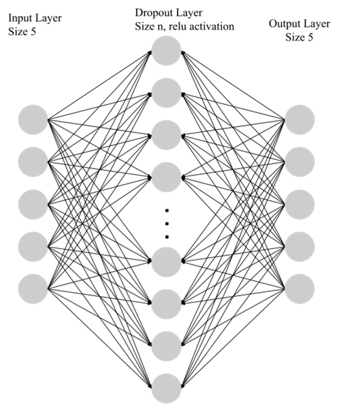
The network architecture was developed, trained, and tested using Python and the PyTorch libraries. Several feedforward fully connected networks with 3, 4, and 5 layers were created and compared. The model began with an input layer, fed with a length 5 vector, corresponding to the 5 |S21| elements (the first layer in Figure 7). This outputs a vector with a constant number of values (the arrows from the first to second layer in Figure 7). The constant was determined during hyperparameter tuning. The second layer applied dropout with probability 10% to the input vector (middle layer in Figure 7). This technique allows the network to ignore some of the input elements and prevents overfitting. Then, the second layer applied the rectified linear unit (ReLu) activation function (middle layer in Figure 7). The third layer took the input vector of the defined constant length, and transformed it back to a length 5 vector, corresponding to the predictions of flexion angles (arrows from middle to last layer in Figure 7). The simplest model, with 3 layers, yielded the most accurate results, with respect to a 3-fold cross validation root-mean-square error (RMSE), based on the smallest difference between actual and predicted angle value. As the modeled problem is simple regression with one input variable, the simple network architecture will be complex enough to see a good level of accuracy. A larger network architecture would be redundant and require unnecessary computation.
The Mean Square Error (MSE) loss function was utilized with the network [31]. This is a common choice for regression models, as the function penalizes large error more heavily, and predictions will converge towards less error. The Adam Optimization Algorithm was chosen [31] which uses both gradient descent and Root-Mean-Square Propagation. The parameter learning rate was determined by a grid search.
During training, for each epoch, an instance of the PyTorch DataLoader object was used to iterate through the training data. In each iteration, data were broken up into mini batches. For each mini batch, gradients of the optimizer were set to 0. Then, the |S21| training vectors were forward propagated through the network to calculate predictions. Finally, loss (MSE) was calculated with the loss function, gradients computed with the optimizer’s backward method, and the optimizer updated using the step method.
During testing, one batch was constructed, with all test data, and |S21| testing vectors were forward propagated through the network to calculate predictions. These predictions were used to calculate error metrics and evaluate the model.

2.3.3. Hyperparameters Tuning

During the grid searching process, the following hyperparameters were chosen to be variable: learning rate, batch size, number of epochs, and layer size [32]. The values searched are shown in Table 3, and as expected, they can have a large impact on the network’s performance, accuracy, and generalization. In the process, each combination of searched values was iterated, and a new ANN was trained and tested using these hyperparameters. Each model was evaluated with a 3-fold cross validation, where for 3 iterations, the model was trained and tested with a new train/test subset of the data. This reduces the effect of any outlier trials.

3. Results

3.1. Evaluation Criteria

Three metrics were chosen to evaluate the model: Coefficient of determination, Root -Mean-Square Error, and relative Root-Mean-Square Error [33]. R is a measure representing the total variance in the dependent variable with respect to the independent variables. RMSE is a measure of the difference between the actual values of the predicted variable and the actual values. rRMSE is a variation of RMSE considering the scale of the predicted variable.

3.2. Assessing Optimal Network Structure and Parameters

After executing the 3-fold cross-validation grid searching process outlined in Section 2.3.3, with the hyperparameter tuning dataset, the hyperparameters shown in Table 4 caused the most optimal error metric (7.35° RMSE). These hyperparameters were used to train all models throughout the rest of this work. This is step 1 in Figure 3.

3.3. Assessing Network Performance

To assess the performance of the chosen model, a 5-fold cross validation was implemented [34]. The cross-validation dataset was utilized for evaluation. Data were previously split into sets per category, so while evaluating error for each fold, RMSE, rRMSE, and R was calculated for all data and each category. These results are seen in Table 5. RMSE for all trials was 7.26°, the largest error was for brisk sleeved trials (RMSE 9.41°), and the smallest error was for jog sleeveless trials (RMSE 5.44°). This is step 2 in Figure 3.
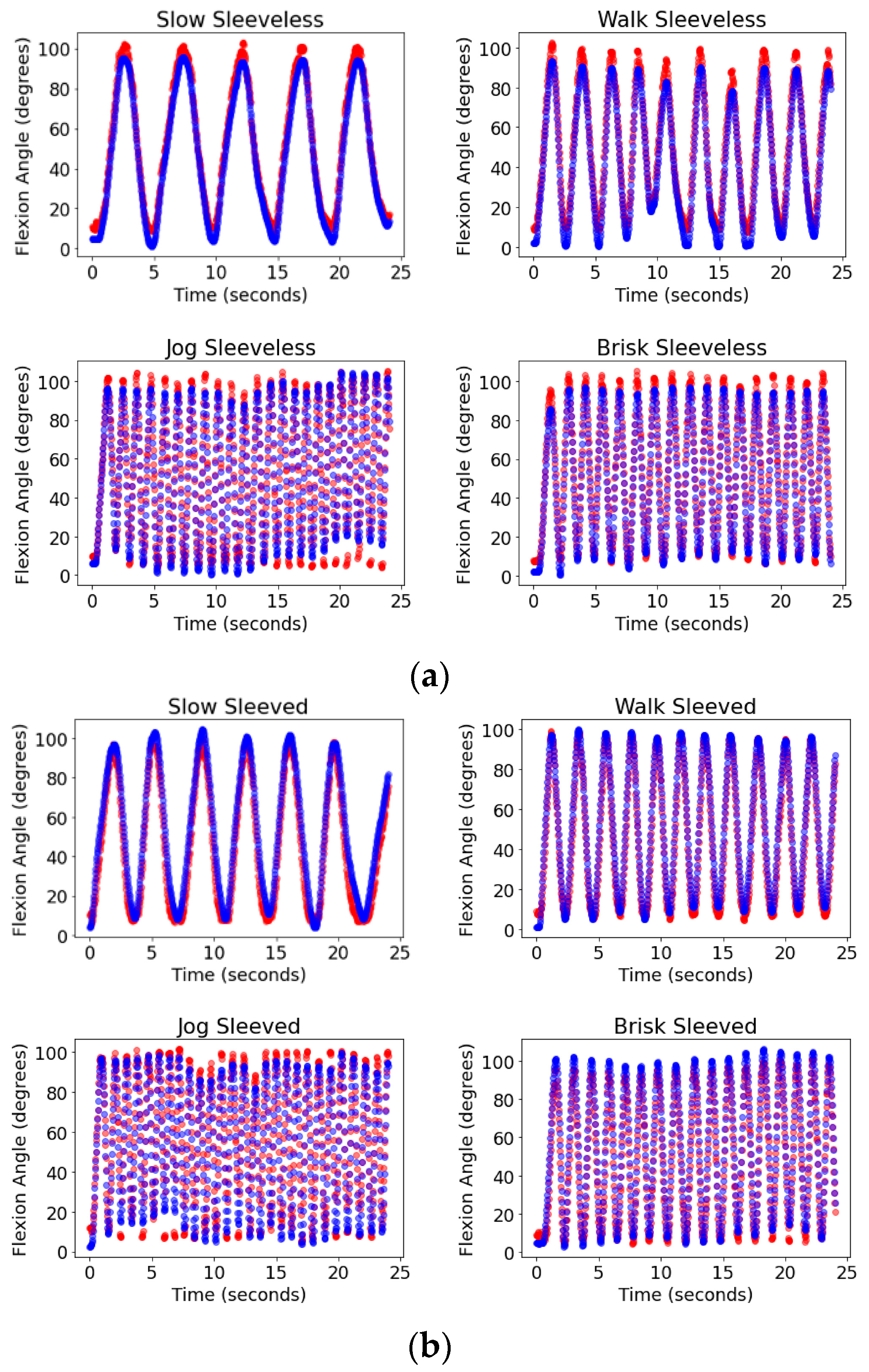
Then, we train the model with the cross-validation dataset, and test with the graphical evaluation dataset. Predicted and actual values were recorded and graphed in the same domain with respect to time [35]. The error results for these trials can be seen in Table 6, and the corresponding predicted vs. actual angle measurements are seen in Figure 8. This is step 3 in Figure 3. From a clinical perspective, different applications would require different levels of angular resolution accuracy. For example, motion capture labs achieve 0.1° in resolution, suitable for even the strictest clinical requirements. However, wearable sensors with RMSE of 3° to 7° have been reported and deemed adequate for several clinical applications [36].

3.4. Comparison to Approaches without Machine Learning

To identify the effectiveness of our model to non-machine learning methods, a simple look-up table based on a Cubic Spline Interpolation method was created and trained on the same data as the model. The reported RMSE values, as shown in Table 7, are much higher than those of our model, which goes to show that machine learning does significantly improve the prediction of flexion angle based on |S21| values.

4. Discussion

4.1. Summary of Reported Phantom-Based Study

The aim of this study was to prove that a machine learning approach could be utilized to effectively predict the relationship between |S21| coefficient and flexion angle. The analysis of the model was divided by category of motion and considered sleeveless and sleeved cases, such that the model’s predictions could be fully understood.
The main finding of the study was that the relationship between |S21| data and flexion angle could be predicted to a reasonable degree of accuracy. The neural network took inputs of data from sensors and made predictions of the angle. It was observed there was no correlation between speed of trial and accuracy of prediction. It was also seen that, for each category of motion, the accuracy of the sleeveless trials was better than the accuracy of the sleeved trials (in terms of RMSE, rRMSE). This suggests that the added noise due to fabrics on the sleeve caused a relationship that was less quantifiable.
In future works, the quality of data collection and optimization of machine learning methods can be improved such that the accuracy of predictions increases for all categories of motion. Referring to Figure 8, we see examples of predicted (blue) vs. actual (red) angles for all speeds as a function of time for sleeveless (Figure 8a) and sleeved (Figure 8b) sensors. It is seen that, especially during the sleeveless model experiments, the error of flexion angle predictions increased when the arm changed direction at high and low angle points. In future works, models can be trained on data that are separated between increasing and decreasing patterns of motion. This may greatly improve accuracy in a similar setting.
During the study, many different models were trained on different subsets of data. The presented architecture was used to train and test a model, for each category, independently of each other. During this experiment, all results yielded an error of RMSE of less than 4°. This level of error is comparable to state-of-the-art wearable technologies, such as 3.3° to 3.6° of error reported for potentiometer-based solutions [37] and 4.3° to 7.1° of error reported for IMU-based solutions [38]. However, these results did not come from a model that was generalized to different types of data. During the process of fine-tuning a machine learning model, it is important to consider the bias variance tradeoff [33]. High bias is caused by fitting an inappropriate model structure to data. High variance is caused by the model reacting to small changes in data and not being generalizable to new inputs. Bias was minimized by comparing several different neural network architectures. Variance was minimized by applying k-fold cross validation and repeatedly ensuring that the model was performing well on unseen data. This also minimized the effects of overfitting.

4.2. Translation to Human Subjects

Our studies have been purposely conducted on phantom models as a proof-of-concept. This is common practice during the first stages of sensor development to establish feasibility in a controlled setup, prior to testing and optimizing on human subjects. In our case, we have demonstrated the improved accuracy of the proposed machine learning approach when training/testing is exclusively conducted on phantom models. We expect our setup to be translatable to human subject data and further improved when a neural network architecture is optimized to infer from high-quality human subject data.
For further validation of real human use cases in this work, we utilize data collected from human subjects as training and testing data in an identical machine learning framework. For this experiment, we utilize data from three human subjects. These data are recorded with the same experimental setup and equipment used on the phantom. The subjects recorded 15, 13, and 18 trials, respectively. Trials included are in the same range of speeds that we measure from the phantom. We implement an analogous machine learning method: data are preprocessed as in Section 2.3.1, then a 5-fold cross validation is performed as in Section 3.3. We utilize the same network architecture and model hyperparameters that we use for evaluation of phantom data.
As seen in Table 8, the new machine learning approach improves the existing one by 0.64 RMSE. This proves that our approach is generalizable for different types of flexion motion from both phantom and human sources. Expectedly, human motion introduces different motion artifacts, such as the impact of a heel strike and skin tissue movement. We assert that the five-point moving average applied will denoise effects of these artifacts. The output vector of length 5 could be filtered in future works to improve accuracy and lessen the effects of artifacts. Additionally, the results we present from human subjects, comparable to the phantom approach, prove that our system can mitigate these artefacts. If a neural network is trained only on human data, motion artifacts are considered.

4.3. Other Study Limitations

As per Table 1, the reported sensor is deemed as “reliable” as (a) it is fabricated using conductive e-threads that have long been validated in terms of mechanical and thermal durability [39], as well as launderability [40], (b) directly specifies angles instead of having to integrate indirect measures of acceleration and/or velocity, and (c) does not deform along with the joint given that loops are placed right above and below the joint instead of right on top of the joint. Nevertheless, longitudinal studies on sensor performance have yet to be performed and are a topic of future research.
Referring to Table 1, we expect the sensor to allow natural motion as it (a) does not interfere with joint motion in any way, and (b) is robust to mechanical and thermal stresses from a fabrication perspective (per our earlier discussion on the use of e-threads). Future human subject studies in real-world environments will include the collection of anecdotal feedback on the sensor’s ability to allow natural motion as well as the associated levels of comfort. Sensor design and selection of materials (fabrics, e-threads) can then be optimized accordingly.
Though our current sensor setup is tethered to a network analyzer, the ultimate goal is a wearable untethered system. In this future implementation, one loop will be connected to a transmitting circuit entailing a 34 MHz crystal oscillator, while the second loop will be connected to a receiving circuit with envelope detection to retrieve the |S21| values. A Bluetooth module will wirelessly transmit the collected measurements to a remote device (e.g., smart phone) for mapping into angles and further post-processing.
Though Table 1 refers to the long-term vision of a wearable technology operating in an unconfined environment, the present study is performed inside a laboratory setting. As sensor development progresses to an untethered setup, both the sensor and associated machine learning approach will be evaluated in real-world environments.
As demonstrated in the past [40], the loop setup of Figure 1 is sensitive not only to joint flexion (sagittal plane) but also rotation (transverse plane). In this feasibility study, we limit phantom motion to the sagittal plane only. In the future, more degrees of motion will be incorporated and sagittal vs. transverse rotation can be decoupled using the three-loop setup reported in [41]. We expect the reported machine learning approach to apply to multi-loop setups as well.
Changing the precise placement of the loops will change the |S21| vs. flexion angle curve shown in Figure 6c. This curve can be learned through calibration for each subject. Alternatively, distance between loops, and placement relative to the joint, could be added as another parameter to the model. Then with appropriate training data, the model can learn the range of |S21| values during a standard flexion, for each distance between loops. If we use this setup with enough subjects and learn calibration patterns for each placement relative to the joint, we could learn the calibration patterns for different types of users. We could also decide on which specific parameters cause significant changes to noise on the curve.

4.4. Potential Applications

When fully implemented in a wearable form factor and used for data collection in real-world environments (i.e., outside the lab and outside the clinic), the proposed sensor system is anticipated to have a major impact in transforming existing healthcare practices. With a focus on the knee joint and without loss of generality, the sensor has the potential to (a) personalize and expedite rehabilitation after injury/surgery (e.g., fractures, dislocations, Anterior Cruciate Ligament Reconstruction), ultimately improving clinical outcomes, (b) provide quantitative/objective measures for return to normal activity and return to play, and (c) optimize athlete training and performance. Beyond the knee, the loop sensor system can also be modified (e.g., number and placement of loops) to monitor motion of other parts of the body, such as the arm, ankle, or the spine. Hence, applications in assessing and optimizing the health of patients, athletes, and the elderly, among others, are expected to be endless.

5. Conclusions

This paper presented a machine learning framework for predicting the flexion angle of a phantom leg, with inputs of transmission coefficient (|S21|) data from wearable loop sensor. This problem was solved in a dynamic setting, where data were collected with respect to time. Speed of data collection was classified between four distinct tasks, and the phantom leg was either sleeved, or sleeveless to study the effects of fabric drift. A multi-step data preprocessing method was employed to put data collected in a comparable domain, and to denoise correlations between inputs and targets. Then, a neural network architecture was utilized as a regression model to predict the flexion angle results. A grid searching process was employed to find optimal hyperparameters for the model. Using a k-fold cross validation evaluation with respect to RMSE, the error of the final model was 7.35 ± 0.34°. Without the proposed neural network method, errors exceeded 35.07° for all scenarios.
In future work, we plan to explore the relationship between |S21| and flexion angle with multiple dimensions of |S21| data from multiple sets of loops on the phantom leg. Additionally, the presented methods can be applied and improved with big data sources from trials of human subjects walking at various speeds, to further this proof of concept. We intend to use human body measurements as features during training such that this method will work for a diverse range of subjects.

Author Contributions

Conceptualization, A.K., M.A.I. and Y.Z.; methodology, A.K., M.A.I. and Y.Z.; software, H.S. and R.R.; validation, H.S. and R.R.; formal analysis, H.S., R.R. and Y.Z.; investigation, H.S., R.R. and Y.Z.; resources, A.K.; data curation, H.S., R.R. and Y.Z.; writing—original draft preparation, H.S.; writing—review and editing, A.K., M.A.I., Y.Z. and R.R.; visualization, H.S. and R.R.; supervision, A.K. and M.A.I.; project administration, A.K.; funding acquisition, A.K. All authors have read and agreed to the published version of the manuscript.

Funding

This research was funded by the U.S. National Science Foundation, grant number 2042644.

Institutional Review Board Statement

All subjects gave their informed consent for inclusion before they participated in the study. The study was conducted in accordance with the Declaration of Helsinki, and the protocol was approved by the Ethics Committee of The Ohio State University (#2017H0472, 08/12/2023).

Informed Consent Statement

Informed consent was obtained from all subjects involved in the study.

Data Availability Statement

Dataset are available on request from the authors.

Acknowledgments

The authors would like to thank undergraduate students Ian Anderson and Chris Cosma for their help in developing the Python-based tool that assisted in data collection and synchronization in this study, and for conducting human subject data collection.

Conflicts of Interest

The authors declare no conflicts of interest.

References

  1. Rovini, E.; Maremmani, C.; Cavallo, F. How Wearable Sensors Can Support Parkinson’s Disease Diagnosis and Treatment: A Systematic Review. Front. Neurosci. 2017, 11, 288959. [Google Scholar] [CrossRef] [PubMed]
  2. Oh, J.; Ripic, Z.; Signorile, J.F.; Andersen, M.S.; Kuenze, C.; Letter, M.; Best, T.M.; Eltoukhy, M. Monitoring joint mechanics in anterior cruciate ligament reconstruction using depth sensor-driven musculoskeletal modeling and statistical parametric mapping. Med. Eng. Phys. 2022, 103, 103796. [Google Scholar] [CrossRef] [PubMed]
  3. Sevick, M.; Eklund, E.; Mensch, A.; Foreman, M.; Standeven, J.; Engsberg, J. Using Free Internet Videogames in Upper Extremity Motor Training for Children with Cerebral Palsy. Behav. Sci. 2016, 6, 10. [Google Scholar] [CrossRef] [PubMed]
  4. Gasparutto, X.; van der Graaff, E.; van der Helm, F.C.T.; Veeger, D.H.E.J. Influence of biomechanical models on joint kinematics and kinetics in baseball pitching. Sports Biomech. 2018, 20, 96–108. [Google Scholar] [CrossRef] [PubMed]
  5. Luu, T.P.; He, Y.; Brown, S.; Nakagome, S.; Contreras-Vidal, J.L. Gait adaptation to visual kinematic perturbations using a real-time closed-loop brain–computer interface to a virtual reality avatar. J. Neural Eng. 2016, 13, 036006. [Google Scholar] [CrossRef] [PubMed]
  6. Xiao, Y.; Zhang, Z.; Beck, A.; Yuan, J.; Thalmann, D. Human–Robot Interaction by Understanding Upper Body Gestures. Presence Virtual Augment. Real. 2014, 23, 133–154. [Google Scholar] [CrossRef]
  7. Jamsrandorj, A.; Kumar, K.S.; Arshad, M.Z.; Mun, K.-R.; Kim, J. Deep Learning Networks for View-independent Knee and Elbow Joint Angle Estimation. In Proceedings of the 2022 44th Annual International Conference of the IEEE Engineering in Medicine & Biology Society (EMBC), Glasgow, UK, 11–15 July 2022; pp. 2703–2707. [Google Scholar] [CrossRef]
  8. Metcalf, C.D.; Robinson, R.; Malpass, A.J.; Bogle, T.P.; Dell, T.A.; Harris, C.; Demain, S.H. Markerless Motion Capture and Measurement of Hand Kinematics: Validation and Application to Home-Based Upper Limb Rehabilitation. IEEE Trans. Biomed. Eng. 2013, 60, 2184–2192. [Google Scholar] [CrossRef] [PubMed]
  9. Zhou, X.; Zhu, M.; Pavlakos, G.; Leonardos, S.; Derpanis, K.G.; Daniilidis, K. MonoCap: Monocular Human Motion Capture using a CNN Coupled with a Geometric Prior. IEEE Trans. Pattern Anal. Mach. Intell. 2018, 41, 901–914. [Google Scholar] [CrossRef] [PubMed]
  10. Sabale, A.S.; Vaidya, Y.M. Accuracy Measurement of Depth Using Kinect Sensor. In Proceedings of the 2016 Conference on Advances in Signal Processing (CASP), Pune, India, 9–11 June 2016; Available online: https://ieeexplore.ieee.org/document/7746156 (accessed on 7 March 2023).
  11. Shin, S.; Li, Z.; Halilaj, E. Markerless Motion Tracking with Noisy Video and IMU Data. IEEE Trans. Biomed. Eng. 2023, 70, 3082–3092. [Google Scholar] [CrossRef]
  12. Bartlett, H.L.; Goldfarb, M. A Phase Variable Approach for IMU-Based Locomotion Activity Recognition. IEEE Trans. Biomed. Eng. 2018, 65, 1330–1338. [Google Scholar] [CrossRef] [PubMed]
  13. Veron-Tocquet, E.; Leboucher, J.; Burdin, V.; Savean, J.; Remy-Neris, O. A Study of Accuracy for a Single Time of Flight Camera Capturing Knee Flexion Movement. In Proceedings of the 2014 IEEE Healthcare Innovation Conference (HIC), Seattle, WA, USA, 8–10 October 2014; Available online: https://ieeexplore.ieee.org/document/7038944 (accessed on 7 March 2023).
  14. Fursattel, P.; Placht, S.; Balda, M.; Schaller, C.; Hofmann, H.; Maier, A.; Riess, C. A Comparative Error Analysis of Current Time-of-Flight Sensors. IEEE Trans. Comput. Imaging 2016, 2, 27–41. [Google Scholar] [CrossRef]
  15. Oubre, B.; Daneault, J.-F.; Boyer, K.; Kim, J.H.; Jasim, M.; Bonato, P.; Lee, S.I. A Simple Low-Cost Wearable Sensor for Long-Term Ambulatory Monitoring of Knee Joint Kinematics. IEEE Trans. Biomed. Eng. 2020, 67, 3483–3490. [Google Scholar] [CrossRef] [PubMed]
  16. Sanca, A.S.; Rocha, J.C.; Eugenio, K.J.S.; Nascimento, L.B.P.; Alsina, P.J. Characterization of Resistive Flex Sensor Applied to Joint Angular Displacement Estimation. In Proceedings of the 2018 Latin American Robotic Symposium, 2018 Brazilian Symposium on Robotics (SBR) and 2018 Workshop on Robotics in Education (WRE), Joȧo Pessoa, Brazil, 6–10 November 2018; Available online: https://ieeexplore.ieee.org/document/8588523 (accessed on 7 March 2023).
  17. Kim, D.; Kwon, J.; Han, S.; Park, Y.-L.; Jo, S. Deep Full-Body Motion Network for a Soft Wearable Motion Sensing Suit. IEEE/ASME Trans. Mechatron. 2019, 24, 56–66. [Google Scholar] [CrossRef]
  18. Li, X.; Wen, R.; Shen, Z.; Wang, Z.; Luk, K.D.K.; Hu, Y. A Wearable Detector for Simultaneous Finger Joint Motion Measurement. IEEE Trans. Biomed. Circuits Syst. 2018, 12, 644–654. [Google Scholar] [CrossRef] [PubMed]
  19. Kobashi, S.; Tsumori, Y.; Imawaki, S.; Yoshiya, S.; Hata, Y. Wearable Knee Kinematics Monitoring System of MARG Sensor and Pressure Sensor Systems. In Proceedings of the 2009 IEEE International Conference on System of Systems Engineering (SoSE), Albuquerque, NM, USA, 30 May–3 June 2009; pp. 1–6. [Google Scholar]
  20. Dai, Z.; Jing, L. Lightweight Extended Kalman Filter for MARG Sensors Attitude Estimation. IEEE Sens. J. 2021, 21, 14749–14758. [Google Scholar] [CrossRef]
  21. Tian, Y.; Wei, H.; Tan, J. An Adaptive-Gain Complementary Filter for Real-Time Human Motion Tracking with MARG Sensors in Free-Living Environments. IEEE Trans. Neural Syst. Rehabil. Eng. 2013, 21, 254–264. [Google Scholar] [CrossRef] [PubMed]
  22. Kun, L.; Inoue, Y.; Shibata, K.; Enguo, C. Ambulatory Estimation of Knee-Joint Kinematics in Anatomical Coordinate System Using Accelerometers and Magnetometers. IEEE Trans. Biomed. Eng. 2011, 58, 435–442. [Google Scholar] [CrossRef] [PubMed]
  23. Mishra, V.; Kiourti, A. Wearable Electrically Small Loop Antennas for Monitoring Joint Kinematics: Guidelines for Optimal Frequency Selection. In Proceedings of the 2020 IEEE International Symposium on Antennas and Propagation and North American Radio Science Meeting, Montreal, QC, Canada, 5–10 July 2020; Available online: https://ieeexplore.ieee.org/document/9329988 (accessed on 7 March 2023).
  24. Mishra, V.; Kiourti, A. Wrap-Around Wearable Coils for Seamless Monitoring of Joint Flexion. IEEE Trans. Biomed. Eng. 2019, 66, 2753–2760. [Google Scholar] [CrossRef] [PubMed]
  25. Ketola, R.; Mishra, V.; Kiourti, A. Modeling Fabric Movement for Future E-Textile Sensors. Sensors 2020, 20, 3735. [Google Scholar] [CrossRef] [PubMed]
  26. Han, Y.; Mishra, V.; Kiourti, A. Denoising Textile Kinematics Sensors: A Machine Learning Approach. In Proceedings of the 3rd URSI Atlantic/Asia-Pacific Radio Science Meeting (URSI AT-AP-RASC), Gran Canaria, Spain, 29 May–3 June 2022; Available online: https://par.nsf.gov/servlets/purl/10354091 (accessed on 9 March 2023).
  27. Zheng, T.; Chen, Z.; Ding, S.; Luo, J. Enhancing RF Sensing with Deep Learning: A Layered Approach. IEEE Commun. Mag. 2021, 59, 70–76. [Google Scholar] [CrossRef]
  28. Bashar, S.K.; Han, D.; Zieneddin, F.; Ding, E.; Fitzgibbons, T.P.; Walkey, A.J.; McManus, D.D.; Javidi, B.; Chon, K.H. Novel Density Poincare Plot Based Machine Learning Method to Detect Atrial Fibrillation from Premature Atrial/Ventricular Contractions. IEEE Trans. Biomed. Eng. 2021, 68, 448–460. [Google Scholar] [CrossRef] [PubMed]
  29. Fitzpatrick, K.; Brewer, M.A.; Turner, S. Another Look at Pedestrian Walking Speed. Transp. Res. Rec. J. Transp. Res. Board 2006, 1982, 21–29. [Google Scholar] [CrossRef]
  30. Barreira, T.V.; Rowe, D.A.; Kang, M. Parameters of Walking and Jogging in Healthy Young Adults. Int. J. Exerc. Sci. 2010, 3, 2. Available online: https://digitalcommons.wku.edu/ijes/vol3/iss1/2/ (accessed on 7 March 2023).
  31. Jia, P.; Liu, H.; Wang, S.; Wang, P. Research on a Mine Gas Concentration Forecasting Model Based on a GRU Network. IEEE Access 2020, 8, 38023–38031. [Google Scholar] [CrossRef]
  32. Panwar, M.; Biswas, D.; Bajaj, H.; Jobges, M.; Turk, R.; Maharatna, K.; Acharyya, A. Rehab-Net: Deep Learning Framework for Arm Movement Classification Using Wearable Sensors for Stroke Rehabilitation. IEEE Trans. Biomed. Eng. 2019, 66, 3026–3037. [Google Scholar] [CrossRef] [PubMed]
  33. Stetter, B.J.; Krafft, F.C.; Ringhof, S.; Stein, T.; Sell, S. A Machine Learning and Wearable Sensor Based Approach to Estimate External Knee Flexion and Adduction Moments During Various Locomotion Tasks. Front. Bioeng. Biotechnol. 2020, 8, 9. [Google Scholar] [CrossRef] [PubMed]
  34. Halilaj, E.; Rajagopal, A.; Fiterau, M.; Hicks, J.L.; Hastie, T.J.; Delp, S.L. Machine learning in human movement biomechanics: Best practices, common pitfalls, and new opportunities. J. Biomech. 2018, 81, 1–11. [Google Scholar] [CrossRef] [PubMed]
  35. Xie, J.; Wang, Q. Benchmarking Machine Learning Algorithms on Blood Glucose Prediction for Type I Diabetes in Comparison with Classical Time-Series Models. IEEE Trans. Biomed. Eng. 2020, 67, 3101–3124. [Google Scholar] [CrossRef] [PubMed]
  36. Zhang, Y.; Caccese, J.B.; Kiourti, A. Wearable Loop Sensor for Bilateral Knee Flexion Monitoring. Sensors 2024, 24, 1549. [Google Scholar] [CrossRef] [PubMed]
  37. Büttner, C.; Milani, T.L.; Sichting, F. Integrating a Potentiometer into a Knee Brace Shows High Potential for Continuous Knee Motion Monitoring. Sensors 2021, 21, 2150. [Google Scholar] [CrossRef]
  38. Slade, P.; Habib, A.; Hicks, J.L.; Delp, S.L. An open-source and wearable system for measuring 3D human motion in real-time. IEEE Trans. Biomed. Eng. 2022, 69, 678–688. [Google Scholar] [CrossRef] [PubMed]
  39. Zhong, J.; Kiourti, A.; Sebastian, T.; Bayram, Y.; Volakis, J.L. Conformal Load-Bearing Spiral Antenna on Conductive Textile Threads. IEEE Antennas Wirel. Propag. Lett. 2016, 16, 230–233. [Google Scholar] [CrossRef]
  40. Toivonen, M.; Bjorninen, T.; Sydanheimo, L.; Ukkonen, L.; Rahmat-Samii, Y. Impact of Moisture and Washing on the Performance of Embroidered UHF RFID Tags. IEEE Antennas Wirel. Propag. Lett. 2013, 12, 1590–1593. [Google Scholar] [CrossRef]
  41. Mishra, V.; Kiourti, A. Wearable Electrically Small Loop Antennas for Monitoring Joint Flexion and Rotation. IEEE Trans. Antennas Propag. 2020, 68, 134–141. [Google Scholar] [CrossRef]
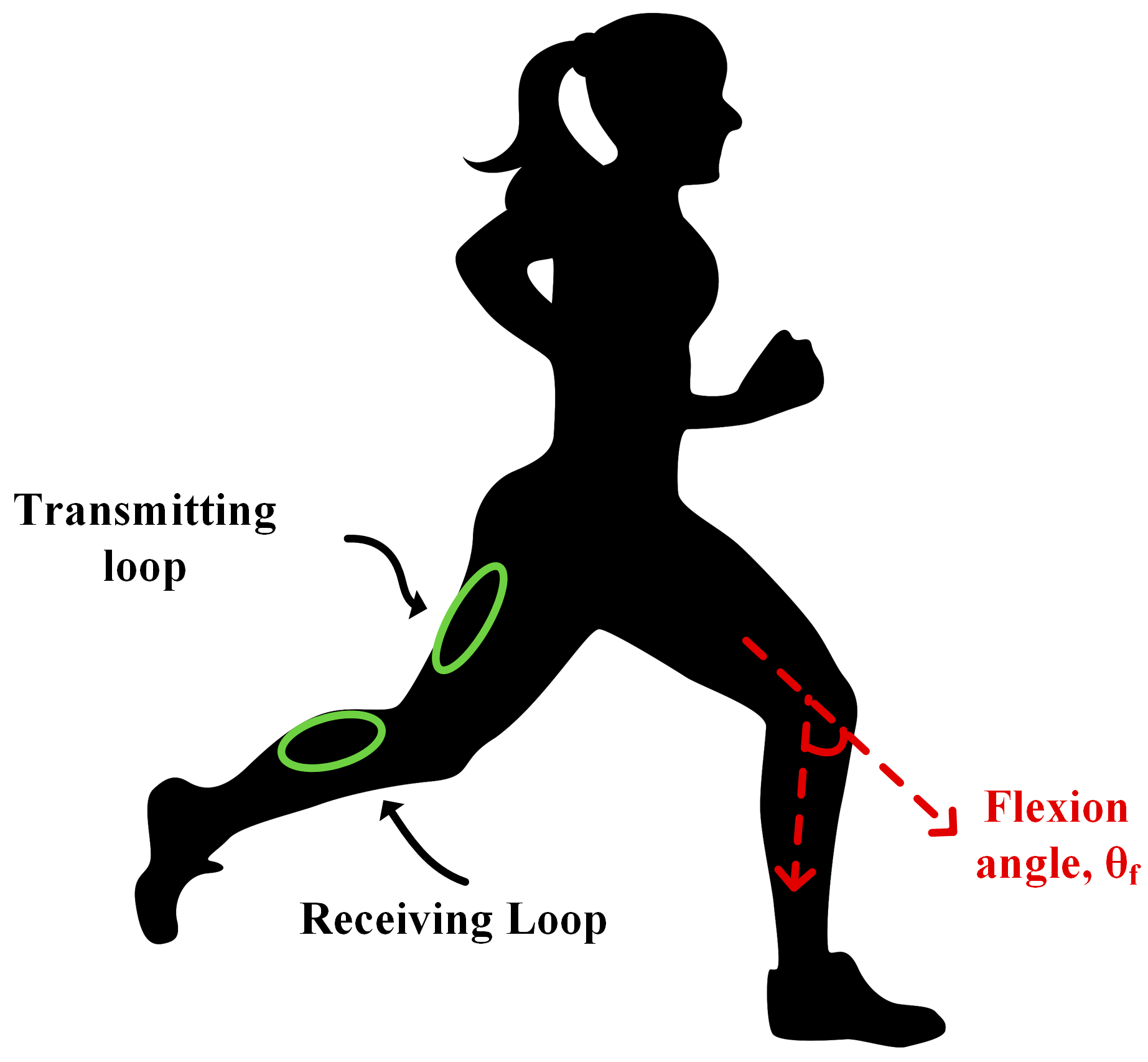
Figure 1. Joint flexion sensor with two planar loops.
Electronics 13 02245 g001
Figure 2. High level flowchart of experiments, data collection, data preprocessing, and machine learning reported in the paper.
Electronics 13 02245 g002
Figure 3. Flowchart describing the machine learning block in Figure 2 higher dimensionality, and it is well known that ANNs are best suited for high-dimensional data.
Electronics 13 02245 g003
Figure 4. Phantoms with two planar loops (one above and one below the joint) employed in this study: (a) sleeveless and (b) sleeved.
Electronics 13 02245 g004
Figure 5. Flowchart describing the data preprocessing block in Figure 2 noise.
Electronics 13 02245 g005
Figure 6. Graphs of |S21| vs time, (camera-measured) angle vs time, sleeveless trials (a), sleeved trials (b), and (camera-measured) angle vs. |S21| for all trials (c).
Electronics 13 02245 g006
Figure 7. Diagram of ANN structure: input, output and feed forward layers.
Electronics 13 02245 g007
Figure 8. Predicted (blue) vs. actual (red) angles as a function of time for all speeds: (a) sleeveless sensor and (b) sleeved sensor.
Electronics 13 02245 g008
Table 1. Comparison of approaches for monitoring joint kinematics.
Camera-Based
[7,8,9,10]
IMUs
[11]
Time-of-Flight
[13,14]
Retractable String
[15]
Bending Sensors
[16,17,18]
MARG Sensor System
[19,20,21]
Magnetometer
[22]
Loop-Based Sensors
(Our Previous Work)
[23,24]
Loop-Based Sensors with Machine Learning
(Proposed)
Works in unconfined environment××
Seamless×××××
Insensitive to line of sight××
Allows natural motion××
Reliable vs. time××××
Low error during dynamic motion××××××
Table 2. Number of flexes per speed.
Motion TypeMotion Speed [m/min]Number of Flexes
SlowN/A3–5
Walking649–13
Brisk Walking8017–19
Jogging11025–30
Table 3. Search values for hyperparameters.
HyperparameterSearched Values
Learning Rate0.001, 0.01, 0.1
Batch Size2, 4, 5
Epochs20, 40
Layer Size1500, 1700, 2000, 2200
Table 4. Optimal hyperparameter values.
HyperparameterChosen Val
Learning Rate0.001
Batch Size2
Epochs40
Layer Size2200
Table 5. Five-Fold cross -validation results.
Motion TypeRMSE (deg)rRMSER
Brisk Sleeved9.41 ± 1.000.17 ± 0.020.98 ± 0.01
Brisk Sleeveless5.90 ± 0.860.12 ± 0.020.99 ± 0.00
Jog Sleeved7.79 ± 0.420.14 ± 0.010.98 ± 0.00
Jog Sleeveless5.44 ± 0.220.11 ± 0.010.99 ± 0.00
Walk Sleeved7.21 ± 0.850.13 ± 0.020.99 ± 0.00
Walk Sleeveless6.11 ± 0.880.13 ± 0.020.99 ± 0.00
Slow Sleeved8.97 ± 0.800.17 ± 0.020.99 ± 0.00
Slow Sleeveless5.90 ± 0.800.12 ± 0.020.99 ± 0.00
All Trials7.26 ± 0.150.14 ± 0.0030.98 ± 0.00
Table 6. Sequential trial results.
Motion TypeRMSE (deg)rRMSER
Brisk Sleeved7.070.130.99
Brisk Sleeveless4.830.100.99
Jog Sleeved5.820.110.99
Jog Sleeveless4.620.090.99
Walk Sleeved6.300.120.99
Walk Sleeveless6.870.160.99
Slow Sleeved8.210.160.99
Slow Sleeveless5.140.110.99
Table 7. RMSE values of non-machine-learning model.
Motion TypeRMSE (deg)
Brisk Sleeved52.00
Brisk Sleeveless46.71
Jog Sleeved51.08
Jog Sleeveless56.53
Walk Sleeved52.15
Walk Sleeveless54.19
Slow Sleeved35.07
Slow Sleeveless44.26
All Trials49.92
Table 8. Human Vs. phantom CV trial results.
ApproachRMSE (deg)rRMSER
Human Trials6.62 ± 0.490.15 ± 0.010.97 ± 0.003
Phantom Trials7.26 ± 0.150.14 ± 0.0030.98 ± 0.001
Disclaimer/Publisher’s Note: The statements, opinions and data contained in all publications are solely those of the individual author(s) and contributor(s) and not of MDPI and/or the editor(s). MDPI and/or the editor(s) disclaim responsibility for any injury to people or property resulting from any ideas, methods, instructions or products referred to in the content.