

Diagnosis Aid System for Colorectal Cancer Using Low Computational Cost Deep Learning Architectures


 , ,
, ,  ,
,  and
and 
Abstract
:1. Introduction
2. Materials and Methods
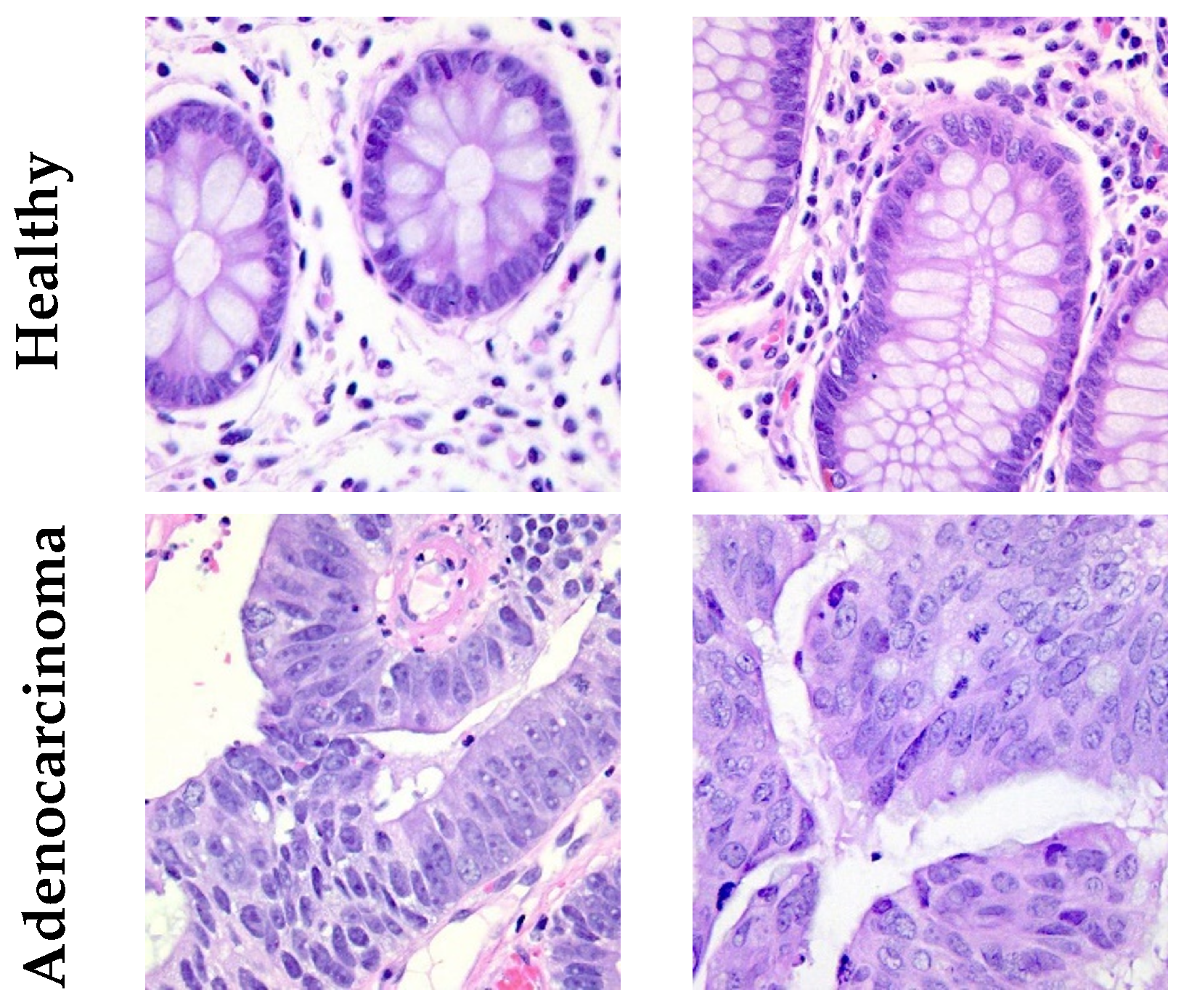
2.1. Dataset
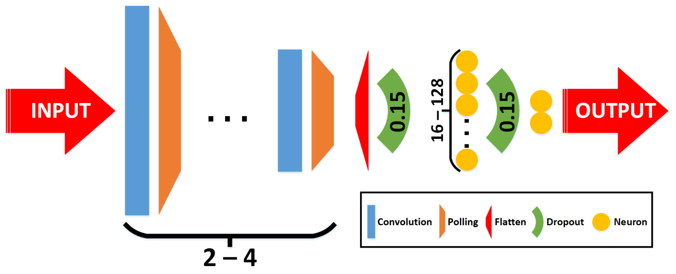
2.2. Classifiers
- Phase 1—grid-search: Multiple combinations of architectures and hyperparameters are used to train the classifiers. In this case, 54 combinations are trained, varying the following parameters:
- –
- Convolutional layers: The number of convolutional layers included in the CNN. This parameter varies with 2 and 4 layers (including a max pooling layer after each one, and a final flatten).
- –
- Image size (pixels): three resolution reductions were tested, specifically 60 × 60, 90 × 90, and 120 × 120.
- –
- Learning rate: Step size at each epoch during the training process to update the connection’s weights. This parameter varies with 1 × , 1 × , and 1 × .
- –
- Batch size: The number of training samples in one forward/backward pass. This parameter varies with 10, 20, and 30.
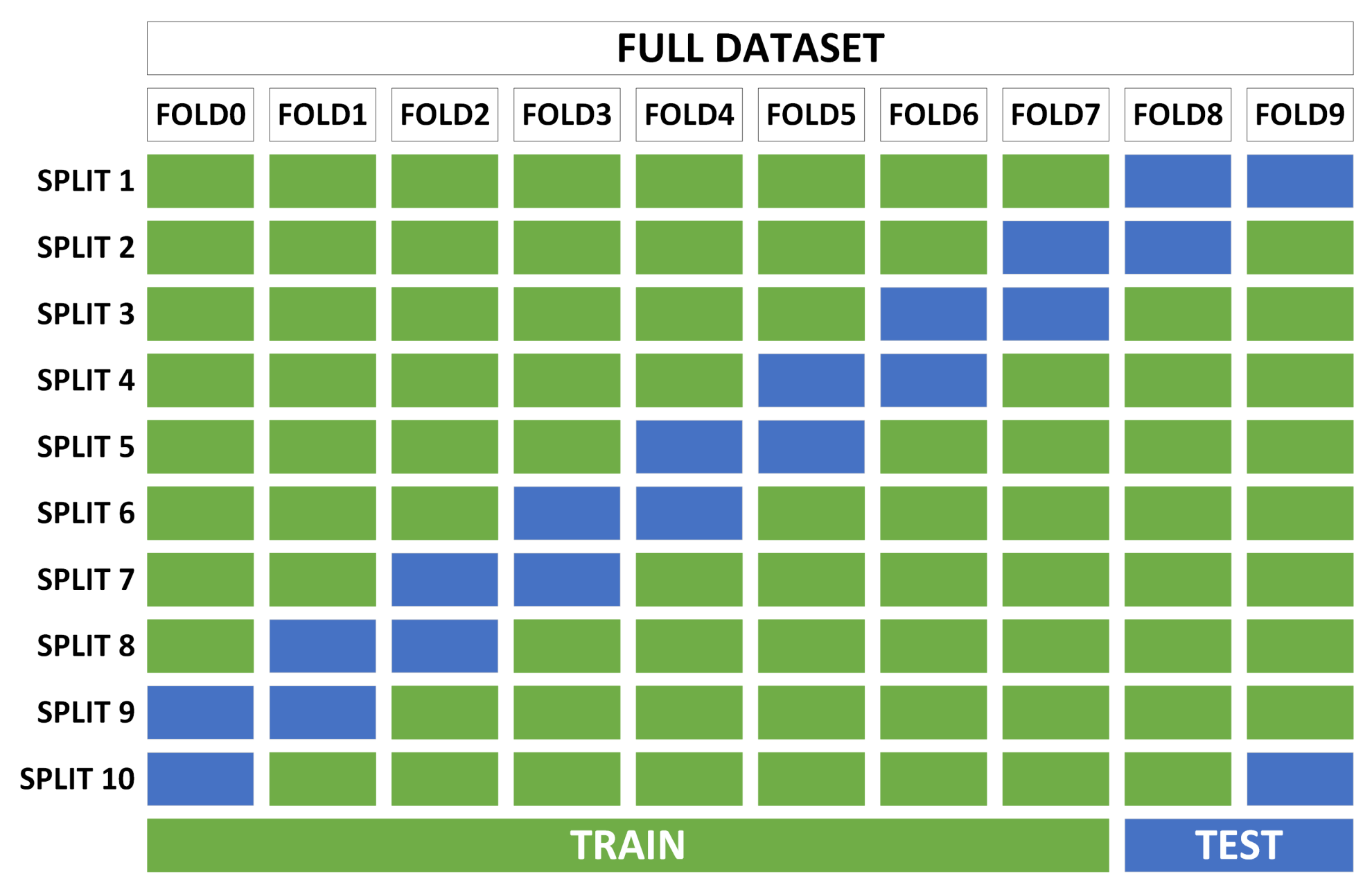
- Phase 2—cross-validation: With the best candidates from the previous search, robustness tests are performed to determine the adaptability of the classifiers to variations in the training and test sets. This process consists of dividing the complete dataset into several non-overlapping subsets and performing several trainings for each classifier, using a specific number of subsets for training and another for testing (different for each training). The standard deviation in the accuracy of all trainings of the same classifier determines the robustness of the classifier.
2.3. Evaluation Metrics
- Accuracy: all samples classified correctly compared to all samples (see Equation (1)).
- Specificity: proportion of “true negative” values in all cases that do not belong to this class (see Equation (2)).
- Precision: proportion of “true positive” values in all cases that have been classified as it (see Equation (3)).
- Sensitivity (or recall): proportion of “True Positive” values in all cases that belong to this class (see Equation (4)).
- : This considers both the precision and the sensitivity (recall) of the test to compute the score. It is the harmonic mean of both parameters (see Equation (5)).
3. Results and Discussion
3.1. Phase 1—Grid-Search
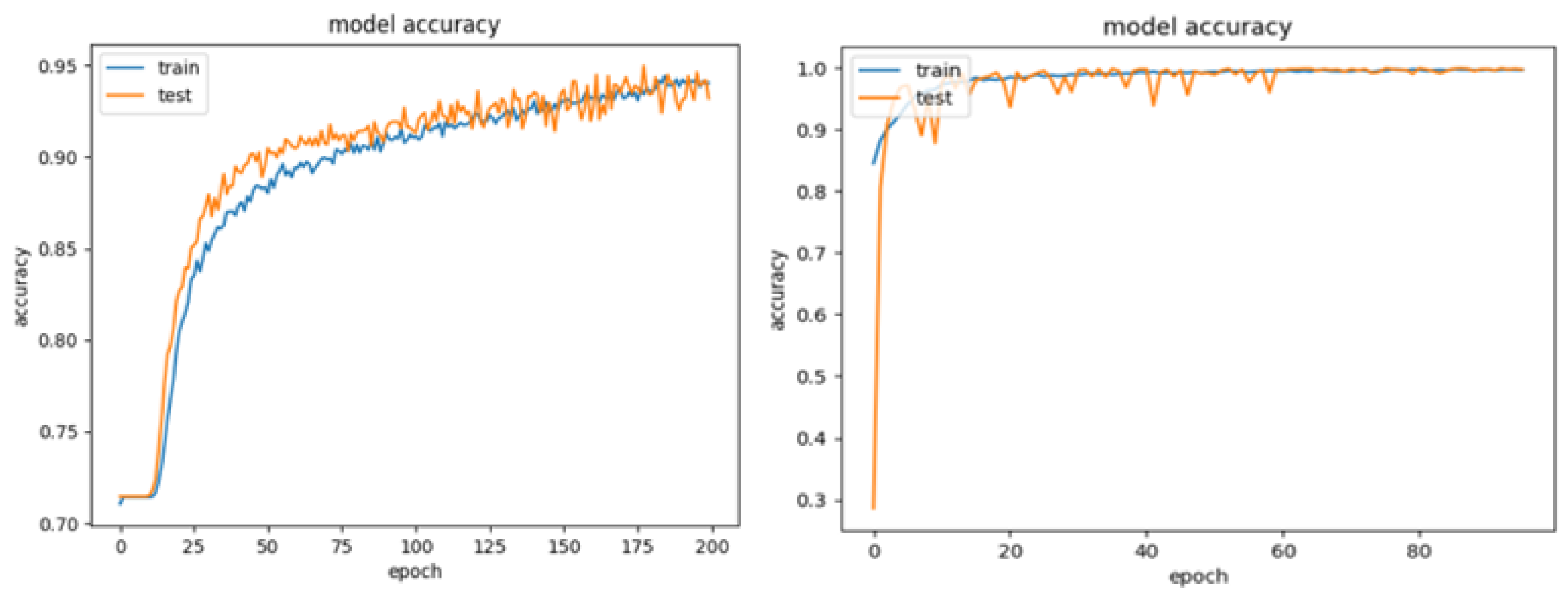
- Candidate 1: Two convolutions, image size 60 × 60 pixels, batch size 10 and learning rate 1 × . Test accuracy results: 95.28%.
- Candidate 2: Four convolutions, image size 60 × 60 pixels, batch size 10 and learning rate 1 × . Test accuracy results: 99.93%.
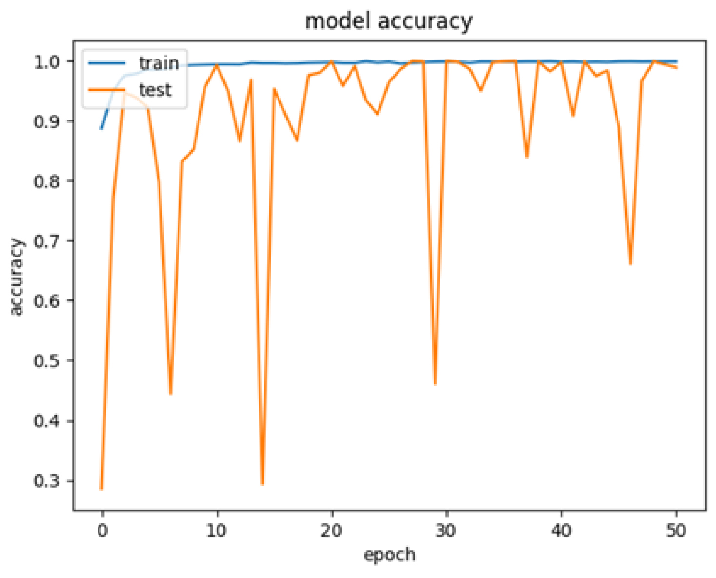
3.2. Phase 2—Cross-Validation
3.3. Comparison to Other Works
4. Conclusions
Author Contributions
Funding
Data Availability Statement
Acknowledgments
Conflicts of Interest
References
- Xi, Y.; Xu, P. Global colorectal cancer burden in 2020 and projections to 2040. Transl. Oncol. 2021, 14, 101174. [Google Scholar] [CrossRef] [PubMed]
- World Health Organization. Colorectal Cancer. 2023. Available online: https://www.iarc.who.int/cancer-type/colorectal-cancer/ (accessed on 12 December 2023).
- American Cancer Society. Invasive Adenocarcinoma. 2023. Available online: https://www.cancer.org/cancer/diagnosis-staging/tests/biopsy-and-cytology-tests/understanding-your-pathology-report/colon-pathology/invasive-adenocarcinoma-of-the-colon.html (accessed on 12 December 2023).
- Clement Santiago, A.; Lubelchek, R. What Does a Pathologist Do? 2024. Available online: https://www.verywellhealth.com/how-to-become-a-pathologist-1736292 (accessed on 29 April 2024).
- Fromer, M.J. Study: Pathology errors can have serious effect on cancer diagnosis & treatment. Oncol. Times 2005, 27, 25–26. [Google Scholar]
- Barber Pérez, P.L.; González-López-Valcárcel, B. Estimación de la Oferta y Demanda de Médicos Especialistas: España 2018–2030. 2019. Available online: https://www.sanidad.gob.es/areas/profesionesSanitarias/profesiones/necesidadEspecialistas/docs/20182030EstimacionOfertaDemandaMedicosEspecialistasV2.pdf (accessed on 29 April 2024).
- Muñoz-Saavedra, L.; Escobar-Linero, E.; Civit-Masot, J.; Luna-Perejón, F.; Civit, A.; Domínguez-Morales, M. A Robust Ensemble of Convolutional Neural Networks for the Detection of Monkeypox Disease from Skin Images. Sensors 2023, 23, 7134. [Google Scholar] [CrossRef] [PubMed]
- Civit-Masot, J.; Bañuls-Beaterio, A.; Domínguez-Morales, M.; Rivas-Pérez, M.; Muñoz-Saavedra, L.; Corral, J.M. Non-small cell lung cancer diagnosis aid with histopathological images using Explainable Deep Learning techniques. Comput. Methods Programs Biomed. 2022, 226, 107108. [Google Scholar] [CrossRef] [PubMed]
- Corral, J.M.; Civit-Masot, J.; Luna-Perejón, F.; Díaz-Cano, I.; Morgado-Estévez, A.; Domínguez-Morales, M. Energy efficiency in edge TPU vs. embedded GPU for computer-aided medical imaging segmentation and classification. Eng. Appl. Artif. Intell. 2024, 127, 107298. [Google Scholar] [CrossRef]
- Civit-Masot, J.; Domínguez-Morales, M.J.; Vicente-Díaz, S.; Civit, A. Dual machine-learning system to aid glaucoma diagnosis using disc and cup feature extraction. IEEE Access 2020, 8, 127519–127529. [Google Scholar] [CrossRef]
- Civit-Masot, J.; Luna-Perejón, F.; Domínguez Morales, M.; Civit, A. Deep learning system for COVID-19 diagnosis aid using X-ray pulmonary images. Appl. Sci. 2020, 10, 4640. [Google Scholar] [CrossRef]
- Muñoz-Saavedra, L.; Civit-Masot, J.; Luna-Perejón, F.; Domínguez-Morales, M.; Civit, A. Does two-class training extract real features? A COVID-19 case study. Appl. Sci. 2021, 11, 1424. [Google Scholar] [CrossRef]
- Hamida, A.B.; Devanne, M.; Weber, J.; Truntzer, C.; Derangère, V.; Ghiringhelli, F.; Forestier, G.; Wemmert, C. Deep learning for colon cancer histopathological images analysis. Comput. Biol. Med. 2021, 136, 104730. [Google Scholar] [CrossRef] [PubMed]
- Singh, O.; Kashyap, K.L.; Singh, K.K. Lung and Colon Cancer Classification of Histopathology Images Using Convolutional Neural Network. SN Comput. Sci. 2024, 5, 223. [Google Scholar] [CrossRef]
- Borkowski, A.A.; Bui, M.M.; Thomas, L.B.; Wilson, C.P.; DeLand, L.A.; Mastorides, S.M. LC25000 Lung and colon Histopathological Image Dataset. arXiv 2019, arXiv:1912.12142. Available online: https://arxiv.org/abs/1912.12142 (accessed on 29 April 2024).
- Sokolova, M.; Lapalme, G. A systematic analysis of performance measures for classification tasks. Inf. Process. Manag. 2009, 45, 427–437. [Google Scholar] [CrossRef]
- Hoo, Z.H.; Candlish, J.; Teare, D. What is an ROC curve? Emerg. Med. J. 2017, 34, 357–359. [Google Scholar] [CrossRef] [PubMed]
- Masud, M.; Sikder, N.; Nahid, A.A.; Bairagi, A.K.; AlZain, M.A. A machine learning approach to diagnosing lung and colon cancer using a deep learning-based classification framework. Sensors 2021, 21, 748. [Google Scholar] [CrossRef] [PubMed]
- Tasnim, Z.; Chakraborty, S.; Shamrat, F.J.; Chowdhury, A.N.; Nuha, H.A.; Karim, A.; Zahir, S.B.; Billah, M.M. Deep learning predictive model for colon cancer patient using CNN-based classification. Int. J. Adv. Comput. Sci. Appl. 2021, 12, 687–696. [Google Scholar] [CrossRef]
- Schiele, S.; Arndt, T.T.; Martin, B.; Miller, S.; Bauer, S.; Banner, B.M.; Brendel, E.M.; Schenkirsch, G.; Anthuber, M.; Huss, R.; et al. Deep learning prediction of metastasis in locally advanced colon cancer using binary histologic tumor images. Cancers 2021, 13, 2074. [Google Scholar] [CrossRef] [PubMed]
- Babu, T.; Singh, T.; Gupta, D.; Hameed, S. Colon cancer prediction on histological images using deep learning features and Bayesian optimized SVM. J. Intell. Fuzzy Syst. 2021, 41, 5275–5286. [Google Scholar] [CrossRef]
- Sakr, A.S.; Soliman, N.F.; Al-Gaashani, M.S.; Pławiak, P.; Ateya, A.A.; Hammad, M. An efficient deep learning approach for colon cancer detection. Appl. Sci. 2022, 12, 8450. [Google Scholar] [CrossRef]
- Ananthakrishnan, B.; Shaik, A.; Chakrabarti, S.; Shukla, V.; Paul, D.; Kavitha, M.S. Smart Diagnosis of Adenocarcinoma Using Convolution Neural Networks and Support Vector Machines. Sustainability 2023, 15, 1399. [Google Scholar] [CrossRef]
- Ravikumar, K.; Kumar, V. CoC-ResNet-classification of colorectal cancer on histopathologic images using residual networks. Multimed. Tools Appl. 2023, 83, 56965–56989. [Google Scholar]


| Class | Train (70%) | Validation (10%) | Test (20%) | TOTAL |
|---|---|---|---|---|
| Healthy | 3500 | 500 | 1000 | 5000 |
| Adenocarcinoma | 3500 | 500 | 1000 | 5000 |
| TOTAL | 7000 | 1000 | 2000 | 10,000 |
| Parameter | Values |
|---|---|
| Convolutional Layers | 2, 4 |
| Kernel size | 3 × 3 |
| Dropout | 0.15 |
| Image size | 60 × 60, 90 × 90, 120 × 120 |
| Learning rate | 1 × , 1 × , 1 × |
| Batch size | 10, 20, 30 |
| Training epochs | 200 |
| Optimizer | Adamax |
| Convolutions | Image Size | Batch Size | Learning Rate | Test Accuracy |
|---|---|---|---|---|
| 2 | 60 × 60 | 10 | 1 × | 99.57% |
| 1 × | 95.28% | |||
| 1 × | 92.99% | |||
| 20 | 1 × | 83.00% | ||
| 1 × | 99.36% | |||
| 1 × | 94.00% | |||
| 30 | 1 × | 97.64% | ||
| 1 × | 93.20% | |||
| 1 × | 92.85% | |||
| 90 × 90 | 10 | 1 × | 97.64% | |
| 1 × | 99.07% | |||
| 1 × | 95.28% | |||
| 20 | 1 × | 32.76% | ||
| 1 × | 84.12% | |||
| 1 × | 93.92% | |||
| 30 | 1 × | 96.57% | ||
| 1 × | 73.39% | |||
| 1 × | 94.13% | |||
| 120 × 120 | 10 | 1 × | 96.47% | |
| 1 × | 98.71% | |||
| 1 × | 94.61% | |||
| 20 | 1 × | 81.00% | ||
| 1 × | 89.74% | |||
| 1 × | 95.11% | |||
| 30 | 1 × | 94.22% | ||
| 1 × | 71.14% | |||
| 1 × | 93.72% | |||
| 4 | 60 × 60 | 10 | 1 × | 98.57% |
| 1 × | 99.93% | |||
| 1 × | 89.91% | |||
| 20 | 1 × | 99.64% | ||
| 1 × | 99.86% | |||
| 1 × | 92.56% | |||
| 30 | 1 × | 99.93% | ||
| 1 × | 99.07% | |||
| 1 × | 99.21% | |||
| 90 × 90 | 10 | 1 × | 96.72% | |
| 1 × | 99.11% | |||
| 1 × | 65.82% | |||
| 20 | 1 × | 99.49% | ||
| 1 × | 99.73% | |||
| 1 × | 67.10% | |||
| 30 | 1 × | 98.72% | ||
| 1 × | 99.68% | |||
| 1 × | 73.95% | |||
| 120 × 120 | 10 | 1 × | 94.42% | |
| 1 × | 99.00% | |||
| 1 × | 47.21% | |||
| 20 | 1 × | 99.30% | ||
| 1 × | 99.93% | |||
| 1 × | 40.00% | |||
| 30 | 1 × | 98.07% | ||
| 1 × | 99.79% | |||
| 1 × | 41.85% |
| FOLD | 1 | 2 | 3 | 4 | 5 | 6 | 7 | 8 | 9 | 10 | Average | STD |
|---|---|---|---|---|---|---|---|---|---|---|---|---|
| Accuracy (%) | 96.04 | 91.43 | 92.14 | 91.79 | 94.29 | 92.14 | 94.29 | 92.86 | 94.29 | 92.81 | 93.2 | 1.46 |
| Loss | 0.1736 | 0.214 | 0.2379 | 0.2125 | 0.1843 | 0.2069 | 0.2041 | 0.1873 | 0.1919 | 0.2347 | 0.204 |
| FOLD | 1 | 2 | 3 | 4 | 5 | 6 | 7 | 8 | 9 | 10 | Average | STD |
|---|---|---|---|---|---|---|---|---|---|---|---|---|
| Accuracy (%) | 100 | 99.29 | 98.21 | 99.64 | 99.64 | 99.64 | 98.57 | 100 | 99.64 | 99.28 | 99.4 | 0.58 |
| Loss | 0.0036 | 0.0179 | 0.0366 | 0.0172 | 0.0076 | 0.0127 | 0.0389 | 0.0063 | 0.0067 | 0.0175 | 0.0165 |
| Class | Accuracy | Specificity | Precision | Sensitivity | F1-Score |
|---|---|---|---|---|---|
| Healthy (HEA) | 100% | 98.24% | 98.27% | 100% | 99.13% |
| Adenocarcinoma (ADE) | 98.24% | 100% | 100% | 98.24% | 99.11% |
| Work | CNN Model | Results | Additional Comments |
|---|---|---|---|
| Hamida et al. [13] (2021) | ResNet (18CL, 6PL, 1DL) SegNet (26CL, 10PL, 1DL) | Acc: 96.77–99.98% Acc: 78.39–99.12% | Same dataset (and others) |
| Masud et al. [18] (2021) | custom (3CL, 3PL, 2DL) | Acc: 96.33% | Same dataset Test subset not considered |
| Tasnim et al. [19] (2021) | MobileNetV2 (+50CL, 1PL, 2DL) | Acc: 95.48–99.67% | Loss: 0.0124 (best) |
| Schiele et al. [20] (2021) | InceptionResNetV2 (25CL, 5PL, 5DL) | Acc: 95% | AUC: 84.2% |
| Babu et al. [21] (2021) | InceptionV3 (+90CL, 15PL, 3DL) | Acc: 96.5–99% | Same dataset (and others) |
| Sakr et al. [22] (2022) | custom (4CL, 4PL, 2DL) | Acc: 99.5% | Same dataset Imags 180 × 180 Test subset not considered |
| Ananthakrishnan et al. [23] (2023) | VGG16 (13CL, 5PL, 2DL) | Acc: 98.6% | Same dataset Test subset not considered |
| Ravikumar and Kumar [24] (2023) | ResNet50V2 (49CL, 2PL, 2DL) | Acc: 99.5% | Same dataset |
| Singh et al. [14] (2024) | DenseNet201 (49CL, 2PL, 2DL) | Acc: 99.12% | Same dataset Test subset not considered |
| This work (2023) | custom (2CL, 2PL, 1DL) custom (4CL, 4PL, 1DL) | Acc: 91.43–96.04% Acc: 98.21–100% |
Disclaimer/Publisher’s Note: The statements, opinions and data contained in all publications are solely those of the individual author(s) and contributor(s) and not of MDPI and/or the editor(s). MDPI and/or the editor(s) disclaim responsibility for any injury to people or property resulting from any ideas, methods, instructions or products referred to in the content. |
© 2024 by the authors. Licensee MDPI, Basel, Switzerland. This article is an open access article distributed under the terms and conditions of the Creative Commons Attribution (CC BY) license (https://creativecommons.org/licenses/by/4.0/).
Share and Cite
Gago-Fabero, Á.; Muñoz-Saavedra, L.; Civit-Masot, J.; Luna-Perejón, F.; Rodríguez Corral, J.M.; Domínguez-Morales, M. Diagnosis Aid System for Colorectal Cancer Using Low Computational Cost Deep Learning Architectures. Electronics 2024, 13, 2248. https://doi.org/10.3390/electronics13122248
Gago-Fabero Á, Muñoz-Saavedra L, Civit-Masot J, Luna-Perejón F, Rodríguez Corral JM, Domínguez-Morales M. Diagnosis Aid System for Colorectal Cancer Using Low Computational Cost Deep Learning Architectures. Electronics. 2024; 13(12):2248. https://doi.org/10.3390/electronics13122248
Chicago/Turabian StyleGago-Fabero, Álvaro, Luis Muñoz-Saavedra, Javier Civit-Masot, Francisco Luna-Perejón, José María Rodríguez Corral, and Manuel Domínguez-Morales. 2024. "Diagnosis Aid System for Colorectal Cancer Using Low Computational Cost Deep Learning Architectures" Electronics 13, no. 12: 2248. https://doi.org/10.3390/electronics13122248