Abstract
Detecting the crystal system of lithium-ion batteries is crucial for optimizing their performance and safety. Understanding the arrangement of atoms or ions within the battery’s electrodes and electrolyte allows for improvements in energy density, cycling stability, and safety features. This knowledge also guides material design and fabrication techniques, driving advancements in battery technology for various applications. In this paper, a publicly available dataset was utilized to develop mathematical equations (MEs) using a genetic programming symbolic classifier (GPSC) to determine the type of crystal structure in Li-ion batteries with a high classification performance. The dataset consists of three different classes transformed into three binary classification datasets using a one-versus-rest approach. Since the target variable of each dataset variation is imbalanced, several oversampling techniques were employed to achieve balanced dataset variations. The GPSC was trained on these balanced dataset variations using a five-fold cross-validation (5FCV) process, and the optimal GPSC hyperparameter values were searched for using a random hyperparameter value search (RHVS) method. The goal was to find the optimal combination of GPSC hyperparameter values to achieve the highest classification performance. After obtaining MEs using the GPSC with the highest classification performance, they were combined and tested on initial binary classification dataset variations. Based on the conducted investigation, the ensemble of MEs could detect the crystal system of Li-ion batteries with a high classification accuracy (1.0).
1. Introduction
The detection of the crystal system in lithium-ion (Li-ion) batteries is crucial for the performance, safety, and longevity of these energy storage devices. The crystal system refers to the arrangement of atoms in the battery’s electrode materials, which significantly influences the electrochemical properties and overall behavior of the battery [1].
Firstly, the crystal structure determines the pathways available for lithium ions to move through the electrode materials during charging and discharging [2]. In materials with a well-ordered crystal structure, such as those with a layered [2] or spinel [3] arrangement, lithium ions can move more easily and predictably. This facilitates a higher ionic conductivity and faster charge–discharge rates, which are essential for applications requiring quick energy delivery and storage, like electric vehicles and portable electronics. Conversely, disordered or less optimal crystal structures can impede the ion mobility, leading to a lower efficiency and capacity.
Secondly, stability of the crystal system under various operating conditions is vital for the battery’s safety and lifespan. Certain crystal structures are more prone to undergoing phase transitions or structural degradation under high voltages, temperature fluctuations, or repeated cycling [4]. These structural changes can cause mechanical stress, leading to the formation of micro-cracks and the eventual failure of the electrode material. By accurately detecting and understanding the crystal system, researchers can design and select materials that maintain the structural integrity over many charge–discharge cycles, thus enhancing the durability and reliability of Li-ion batteries [5].
Furthermore, the crystal system influences the battery’s capacity and energy density. High-capacity electrode materials, such as those based on lithium-rich layered oxides, rely on specific crystal structures to accommodate a higher number of lithium ions per unit volume or mass [6]. Detecting and optimizing these crystal structures can lead to the development of batteries with higher energy densities, which is a key factor in extending the range of electric vehicles and the battery life of portable devices.
Lastly, advanced characterization techniques used to detect crystal systems, such as X-ray diffraction (XRD) and transmission electron microscopy (TEM), provide detailed insights into the atomic-scale arrangement and any defects or impurities present. This information is critical for improving the synthesis and processing methods of electrode materials, ensuring that the desired crystal structure is achieved consistently in large-scale production. The concept of pseudocapacitance was proposed in [7] as a rapid method for determining the state of health (SOH) of batteries and supercapacitors, offering an alternative to traditional full charge/discharge cycle degradation analysis. Impedance spectroscopy is used to study various lithium-ion and sodium-ion batteries and supercapacitors, distinguishing Faradaic and capacitive charge storage and suggesting new diagnostic diagrams for instant performance and failure analyses.
Another important element in Li-ion batteries is separators, which are crucial because they prevent physical contact between the anode and cathode, thereby avoiding short circuits while allowing ions to pass through to facilitate electrochemical reactions. Their properties directly affect the battery’s safety, performance, and longevity. In [8], fluorinated polyimide (FPI) was synthesized and blended with polyvinylidene fluoride (PVDF) to fabricate composite nanofibrous membranes (CNMs) via the electrospinning method. The investigation showed that the prepared CNMs provide an innovative and promising approach to the development and design of high-performance separators. In [9], transition metal vanadates (TMVs) were synthesized directly on current collectors on the nanoscale, which enhanced the performance, particularly in Li-ion batteries and catalytic applications. A novel and facile method was developed in [10] to synthesize zinc tin sulfide@reduced graphene oxide (ZnSnS3@rGO), exhibiting an excellent sodium- and lithium-ion storage performance with a high specific capacity, rate capability, and cycle life. Highly safe and stable wide-temperature operation is critical for lithium metal batteries (LMBs). An amide-based eutectic electrolyte composed of N-methyl-2,2,2-trifluoroacetamide (NMTFA) and lithium difluoro(oxalato)borate has been designed in [11], enabling LMBs to operate from 25 °C to 100 °C with a fast charging performance, high thermal tolerance, non-flammability, and enhanced capacity retention after extensive cycling at high temperatures. Graphite anodes are susceptible to dangerous Li plating during fast charging, but identifying the rate-limiting step has been challenging. By introducing a triglyme (G3)-LiNO3 synergistic additive (GLN) to a commercial carbonate electrolyte in [12], an elastic solid electrolyte interphase (SEI) with a uniform Li-ion flux was constructed, achieving dendrite-free, highly reversible Li plating and enhancing the stability and uniformity of Li deposition, resulting in a 99.6% Li plating reversibility over 100 cycles and stable operation of a 1.2 Ah LiFePO4|graphite pouch cell over 150 cycles at 3 °C.
In summary, the detection of the crystal system in Li-ion batteries is a foundational aspect of enhancing their performance, safety, and longevity [5]. It enables the optimization of ionic conductivity, structural stability, capacity, and energy density, which are all crucial for meeting the increasing demands of modern energy storage applications.
In the last decade, several research papers have investigated the possibility of using artificial intelligence to see if these algorithms could detect the crystal system of Li-ion batteries with a high classification accuracy. The progress and recent advancements in machine learning tools tailored for improving battery materials, management strategies, and system–system-level optimization are well documented in [13].
In [14], the authors used linear discriminant analysis (LDA), quadratic discriminant analysis (QDA), shrinkage discriminant analysis (SDA), artificial neural networks (ANNs), support vector machines (SVMs), k-nearest neighbor (kNN), random forest (RF), and extremely randomized trees (ERTs) for Li-ion crystal structure classification. The highest average accuracy of 75% was achieved using the RF and ERT methods. KNN was used in [15] for the classification of the crystal structure of Li-ion batteries. This investigation showed that the model can predict the crystalline group of the test compound with an accuracy higher than 80% and a precision higher than 90%. A deep neural network was used for the classification of a Li-ion battery crystal system. For comparison, the authors used SVM, logistic regression (LR), naive Bayes (NB), and a voting ensemble (VE) consisting of SVM, LR, and NB. The classification performance was measured using the precision, recall, and F1-score. The highest classification performance was achieved using a DNN with a macro precision, recall, and F1-score of 0.82, 0.82, and 0.81, respectively. In Table 1, the previous research methods and results are summarized.

Table 1.
A summary of the literature.
The main problem with the previously described research is that the majority of it used artificial intelligence (AI) methods that could not be transformed into mathematical equations that could be used for the detection of crystal systems with a high classification performance. This is especially valid for neural networks, which cannot be transformed into mathematical equations due to the large number of mutually connected neurons. The other problem with these trained algorithms is that they require a substantial amount of memory to be stored and computational power to be applied to new samples.
The idea behind this paper is to see if a genetic programming symbolic classifier (GPSC) could be applied to obtain mathematical equations (MEs) that could detect a crystal system with a high classification performance. For this investigation, a publicly available dataset was used with a target multiclass that is imbalanced. The first step is to transform the multiclass dataset into a multiple binary dataset using a one-versus-rest approach, and, by doing so, multiple imbalanced dataset variations will be obtained. To address this problem, several oversampling techniques were considered to obtain balanced dataset variations which could be used in the GPSC to obtain MEs. Another problem that arises is the large number of GPSC hyperparameters, and the goal is to find the optimal combination of GPSC hyperparameter values for which the GPSC can generate MEs with a high classification performance. The optimal combination of GPSC hyperparameter values will be searched for using the random hyperparameter value search (RHVS) method. To obtain a robust system of MEs, the five-fold cross-validation (5FCV) training method was used, since for each split of 5FCV, one ME is obtained, totaling five MEs in one training with 5FCV. After the best MEs are obtained from balanced dataset variations, these MEs will be combined together in a threshold-based voting ensemble. The idea is to find the threshold at which the classification performance is the highest and to determine whether using a threshold-based voting ensemble improves the classification performance.
The novelty of this paper is the proposal of a procedure through which MEs can be easily obtained and that can detect the crystal structure of Li-ion batteries. Based on the problem description (importance of crystal system detection), the overview of the literature, and the idea/novelty in this paper, the following questions arise:
- Is it possible to obtain MEs with the GPSC that can detect the crystal system type of Li-ion batteries with a high classification performance?
- Can the application of oversampling techniques achieve a balance between class samples, and can using these balanced dataset variations in the GPSC produce MEs with a high classification performance?
- Can the application of the RHVS method find the optimal combination of GPSC hyperparameters for each balanced dataset variation which can generate highly accurate MEs?
- Can the application of 5FCV produce a robust system of MEs with a high classification performance?
- Can a combination of MEs obtained by the GPSC in an ensemble produce even an higher classification performance in the detection of Li-ion batteries?
The paper comprises sections on Materials and Methods, Results, Discussion, and Conclusions. The Materials and Methods detail the research approach, dataset, statistical analysis, oversampling process, classifier setup, evaluation process, and ensemble method. The results include the best MEs on balanced datasets, GPSC hyperparameters, and classification performances. The Discussion interprets the results for deriving conclusions. The Conclusions summarizes the research, hypothesis outcomes, pros, cons, and future directions. The Appendix A provides modified mathematical functions for the GPSC and instructions for accessing MEs.
2. Materials and Methods
This section begins with the research methodology, which is followed by descriptions of the dataset, oversampling techniques and their applications, the genetic programming symbolic classifier with the random hyperparameter search method, evaluation metrics, the train–test procedure, and the threshold-based voting ensemble.
2.1. Research Methodology
The research methodology consists of the following steps:
- 1.
- An initial statistical investigation of the dataset, preprocessing, and creation of balanced dataset variations using various oversampling techniques;
- 2.
- Application of the GPSC with the RHVS method trained with 5FCV on each balanced dataset variation to find the best MEs using the optimal combination of GPSC hyperparameters;
- 3.
- Combination of the best MEs in a threshold-based voting ensemble and an evaluation of the initial dataset to find the threshold value at which the classification performance is the highest.
A graphical representation of the research methodology is shown in Figure 1.
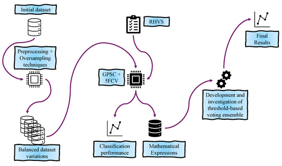
Figure 1.
The graphical representation of research methodology.
2.2. Dataset Description and Statistical Analysis
The dataset used in this research is publicly available on Kaggle (the dataset link is given in Data Availability). The dataset consists of 11 variables (columns) with 339 samples in total. The initial problem with the dataset is that some variables contain only string values, and they were transformed into a numeric format using a label encoder (simple sklearn library preprocessing function). However, the first variable, Material ID, was removed from the dataset and underwent further investigation since the variable values are a sequence of numbers with the prefix “mp-” and are not relevant to the research. In Table 2, the transformation of each string variable to numeric format using abel encoder is shown.
Table 2.
The variables in initial dataset that contained string values and their integer values after application of the label encoder.
As seen from Table 2, Formulas, Spacegroup, Has Bandstructure, and Crystal System were the variables that initially contained string values and were transformed to the integer type using the label encoder. One of the concerns with the Formula variable is that the approach used here is rather simple and unconventional. Due to the small/limited number of chemical compounds which are used for Li-ion batteries, the idea of using the label encoder is pretty straightforward. The output variable, Crystal System, consists of three classes (multi-class problem), i.e., monoclinic, orthorhombic, and triclinic. The label encoder assigned monoclinic to class_0, orthorhombic to class_1, and triclinic to class_2. However, further investigation should uncover if the dataset is imbalanced. Now that all variables are in a numeric format, the results of an initial statistical analysis, i.e., calculation of minimum, maximum, mean, standard deviation, and number of samples for each variable, are obtained and shown in Table 3.
Table 3.
The results of the dataset’s basic statistical analysis.
As seen from Table 3, it can be noted that there are a total of 10 variables, where 9 of these variables are input variables which are in the GPSC, represented as ,……,, while 1 target variable is Crystal System, represented in the GPSC as y. The input variables used in this research are:
- 1.
- Chemical Formula—this is the notation that represents the elements present in the materials and their proportions (e.g., LiFePO4). It provides essential information about the material’s composition. Since there are a small number of chemical formulas in this dataset, as indicated previously, they were all transformed from a string value to an integer value using the label encoder.
- 2.
- Spacegroup—this variable describes the symmetry group of the crystal structure. It is a classification that reflects the symmetrical properties of the crystal lattice, important for understanding its geometric properties.
- 3.
- Formation Energy—the energy change that occurs when a compound is formed from its constituent elements. This is often measured in electron volts (eV) and indicates the stability of the compound.
- 4.
- E Above Hull (eV)—this represents the energy of the material relative to the most stable phase (convex hull) in a phase diagram. A lower E Above Hull value indicates a more stable material.
- 5.
- Band Gap (eV)—this variable represents the energy difference between the valence band and the conduction band in the material. This property determines the material’s electrical conductivity and is measured in electron volts (eV).
- 6.
- N Sites—the number of unique atomic sites in the unit cell of the crystal structure. This reflects the complexity of the crystal lattice.
- 7.
- Density (g/cc)—the mass per unit volume of the material, measured in grams per cubic centimeter. It is a fundamental physical property influencing the material’s mechanical and thermal characteristics.
- 8.
- Volume—this variable represents the volume of the unit cell of the crystal structure, typically measured in cubic angstroms. This gives an idea of the spatial dimensions of the crystal lattice.
- 9.
- Has Bandstructure—this variable was initially a Boolean variable and was converted to 0 or 1 using the label encoder. This variable indicates whether the band structure of the material is known and available. Has Bandstructure provides crucial information about the electronic properties of the material.
- 10.
- Crystal System—this is the target variable that initially consists of three values, i.e., monoclinic, orthorhombic, and triclinic, and was transformed to integer values (0, 1, and 2) again using the label encoder. Each of the crystal structures refers to the arrangement of atoms in the crystal lattice, which defines the overall geometric and symmetry properties of the material.
- Monoclinic crystal structure—one of the seven crystal systems in crystallography. The crystal structure is characterized by three unequal axes (a, b, and c), where two axes (a and c) are not perpendicular to each other but the third axis (b) is perpendicular to the plane formed by the other two. The angles between axes are 90° and 90°. This type of crystal system has a lower symmetry compared to other systems like cubic or hexagonal systems. It generally has one two-fold rotation axis or one mirror plane.
- Orthorhombic crystal structure—this structure has three mutually perpendicular axes (a, b, and c) of different lengths (). All angles between the axes are 90°. The orthorhombic system has a higher symmetry than the monoclinic system but a lower symmetry than cubic or hexagonal systems. It has three two-fold rotational symmetry axes or three mirror planes.
- Triclinic crystal structure—this structure has three axes (a, b, and c) of different lengths () that are not perpendicular to each other. All angles between the axes are different and none are 90°. The crystal system has the least symmetry among all crystal systems, often only possessing a center of inversion symmetry.
From Table 3, it can be seen that all dataset variables have the same number of samples (count = 339), so no values are missing. The main problem with the dataset can be seen by examining the mean and std values of the target (Crystal System) variable. The mean value is equal to 0.80236, which could indicate that there are more samples in class_0 and class_1 and a smaller number of samples in class_2. This analysis indicates that the multi-class dataset is imbalanced. The number of samples for each class is shown in Figure 2.
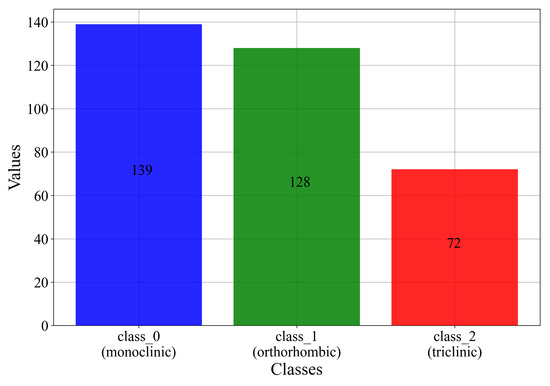
Figure 2.
The initial number of samples for each class.
As seen from Figure 2, class_0 contains the largest number of samples (139). class_1 has a slightly lower number of samples (128), while class_2 has the lowest number of samples (72). From this investigation, it can be noted that the dataset is greatly imbalanced, and due to a lower total number of samples, it must be synthetically balanced using oversampling techniques.
Since the GPSC cannot solve the multiclass problem, the dataset will be divided manually into three initial datasets for detection of class_0, class_1, and class_2 cases. This is the one-versus-rest approach, only it is performed manually. The comparison of the target variable in each dataset is shown in Figure 3.

Figure 3.
The bar plot showing class_0–2 in one-versus-rest approach.
To perform the one-versus-rest approach manually for each class, an additional column must be created in the dataset file (.csv file), and every sample that does not belong to the class is labeled 0, while each sample that belongs to the class is labeled as 1. From Figure 3, it can be noted that all the classes are still imbalanced and that the application of oversampling techniques would be necessary. Next, a Pearson’s correlation analysis was conducted between input and target variables to assess the correlation strength. The correlation coefficient ranges from −1 to 1 [17]: 1 signifies a perfect positive correlation, −1 indicates a perfect negative correlation, and 0 reflects no correlation. The results are depicted in Figure 4.
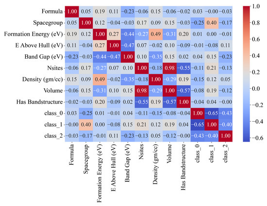
Figure 4.
The Pearson’s correlation analysis represented in the form of a heatmap.
As seen from Figure 4, class_0 has the lowest negative correlation with the Spacegroup variable (−0.25), and the other variables have a very small negative or positive correlation in the −0.15 to 0.04 range. The correlations with class_1 and class_2 variables are not important, since all input variables with each of the classes will be used in the GPSC separately. The class_1 variable has a relatively good positive correlation with Spacegroup (0.4) followed by Nsites (0.21). All other variables have a correlation in the −0.077 to 0.15 range. class_2 has a correlation of −0.23 to 0.11. Generally, the correlation values between the input variables and the output variables are very small.
The next step is the perform an outlier detection analysis, since the large number of outliers has a great influence on the classification performance of the trained ML method. Outlier detection is crucial in data analysis for maintaining the data integrity, enhancing the model’s performance, uncovering insights, and ensuring the validity of statistical assumptions. Outliers can result from errors in data collection or entry, and addressing them helps maintain the accuracy of the dataset. They can also skew statistical analyses and machine learning models, leading to inaccurate predictions and a poor performance. Detecting and handling outliers ensure more reliable and robust models. Additionally, outliers might represent significant but rare events or conditions, providing valuable insights into underlying phenomena that could otherwise be overlooked.
Boxplot analysis is a powerful graphical tool that aids in visualizing data distributions, detecting outliers, comparing groups, and summarizing data effectively. A box plot provides a summary of the data distribution, highlighting the median, quartiles, and overall spread, which helps in understanding the central tendency and variability at a glance. It clearly indicates outliers as points outside the whiskers, making it easy to identify anomalies. Box plots are also useful for comparing distributions across different groups, helping to understand differences, identify trends, and guide further analysis. By summarizing key statistical measures concisely, box plots facilitate effective communication of findings and insights. The distribution of each variable is graphically shown in Figure 5.
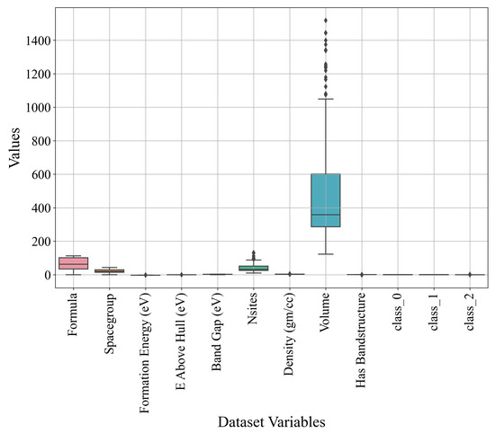
Figure 5.
The box plot showing the distribution of variable values.
From Figure 5, it can be noted that the majority of variables do not have outliers, with the exception of the Nsites and Volume variables. The number of outliers (15 and 19) can be determined by the Nsites and Volume variables. The range of values for the majority of the variables is in the 0 to 150 range. However, the Volume variable values are between 150 and almost 1500 (outliers included). An outlier analysis suggests that some outlier capping or removal techniques should be applied. However, in this research, the idea is to see if the GPSC could generate MEs with a high classification performance using the original range of input variables with outliers.
2.3. Application of Oversampling Techniques
An imbalanced dataset can have a great impact on the classification performance of machine learning (ML)-trained models. So, it is generally good practice to somehow achieve a balance between classes. In binary classification, the imbalanced dataset has two classes, where one, with a higher number of samples, is the majority class and the other is the minority class. The idea of using oversampling techniques is to either reduce the number of majority class samples to the number of minority class samples using undersampling techniques or to increase the number of minority class samples to the number of majority class samples using oversampling techniques. The problem with undersampling techniques is that usually, they take a longer time to achieve a balance and the parameters of undersampling techniques have to be finely tuned to achieve this balance. Oversampling techniques usually achieve a balance between classes quickly, and parameter tuning for oversampling techniques is usually not required. So, for these reasons, in this investigation, oversampling techniques were applied, and these were ADASYN, BorderlineSMOTE, KMeansSMOTE, SMOTE, and SVMSMOTE.
2.3.1. ADASYN
The adaptive synthetic (ADASYN) technique [18] is an oversampling technique used in the field of ML to address the issue of class imbalance in the dataset. Class imbalance occurs when one class has a higher number of samples than the other class. This imbalance can lead to a biased ML model classification performance, favoring the majority class. The primary objective of the ADASYN technique is to improve the ML classifier performance on the minority class by generating synthetic data samples. This technique adapts to the data distribution, focusing more on generating samples in regions where the minority class is sparsely separated. The ADASYN technique consists of the following steps:
- 1.
- Calculate the class imbalance—for the initial imbalanced dataset, determine the minority (lower number of samples) and majority class (higher number of samples). Then, ADASYN calculates the ratio of the minority class to the majority class. This ratio is important to understand the degree of imbalance.
- 2.
- Compute K-nearest neighbors (KNNs)—for each minority class, the sample calculates the K-nearest neighbors (default k = 5). Identify how many of these neighbors belong to the majority class.
- 3.
- Compute distribution density—determine the density distribution for each minority class sample based on the proportion of majority class neighbors. This step is necessary to identify samples that are in regions with a higher class imbalance.
- 4.
- Determine the number of synthetic samples.
- 5.
- Generate synthetic samples.
2.3.2. BorderlineSMOTE
BorderlineSMOTE (Borderline Synthetic Minority Oversampling Technique) is an extension of the SMOTE technique used to address the class imbalance in ML datasets [19]. The idea of BorderlineSMOTE is to generate synthetic samples of the minority class by interpolating between existing samples. The SMOTE technique can sometimes generate noisy samples, especially in regions where the minority class is spread sparsely or overlaps with the majority class. The BorderlineSMOTE technique solves this problem, since it is focused on samples that are close to the decision boundary between classes. This technique consists of three steps and these are:
- Identify borderline instances: this technique first identifies minority class samples that are near the decision boundary, i.e., those samples that have majority class samples in their neighborhood.
- Selectively generate synthetic samples: Instead of generating synthetic samples for all minority class samples like in the SMOTE technique, the BorderlineSMOTE technique is focused on borderline samples only. This technique generates synthetic samples by randomly selecting the minority class sample and then selecting one of its nearest minority class neighbors. The synthetic sample is then generated along the line that connects the two samples, within a specified range.
- Address class imbalance: the synthetic samples are added to the minority class and thus a balance between the majority and minority class is achieved.
The benefit of generating synthetic samples near the decision boundary is that it improves the generalization performance of the classifier, since the technique focuses on regions where the classifier is likely to make errors. Eventually, this can lead to a better classification performance when compared to traditional SMOTE, especially in cases where the minority class is sparsely distributed and overlaps with the majority class.
2.3.3. KMeansSMOTE
The KMeansSMOTE (KMeans Synthetic Minority Oversampling Technique) is another variation of the SMOTE technique that combines K-Means clustering with the SMOTE technique to address class imbalances in the dataset [20]. The goal of this technique is to achieve a balanced dataset by oversampling minority classes to achieve a similar or equal number of majority class samples by leveraging the clustering information provided by K-Means. KMeansSMOTE consists of the following steps:
- 1.
- Cluster the minority class samples—After the minority and majority classes are identified, the minority class samples are grouped into k clusters. The number of k clusters can be chosen based on the dataset characteristics or using methods like the elbow method. For each cluster, K-Means identifies a centroid, which represents the center of the cluster. However, in this investigation, the number of k is set to None and instead, the MiniBatchKMeans algorithm was used. This algorithm is a variant of the K-Means clustering algorithm which is designed to handle large datasets more efficiently. The algorithm achieves this by using small, random subsets (mini-batches) of the data to update the cluster centroids incrementally, rather than using the entire dataset. This approach reduces the computational complexity and memory usage, making it suitable for large-scale data.
- 2.
- Balance the clusters—The number of synthetic samples that must be synthetically generated to balance the dataset or to achieve the desired minority-to-majority class ratio is calculated. Then, the technique distributes the required number of samples across the clusters, often proportionally based on the size of each cluster based on the cluster’s density.
- 3.
- Generate synthetic samples—For each cluster, pairs of minority class samples are selected to generate synthetic samples. Then, synthetic samples are generated by interpolating between selected pairs of samples within the same cluster. This interpolation process involves creating new samples along the line segments connecting two samples, similar to the original SMOTE technique but applied to each cluster.
- 4.
- Balancing the dataset: The generated synthetic samples are added to the minority class, which increases its size and thus balances the class distribution.
The benefits of using KMeansSMOTE are the localized synthetic generation, the improved decision boundaries, and its ability to handle complex distributions. Localized synthetic generation is achieved by generating synthetic samples within clusters. This way, the technique ensures that synthetic samples are more representative of the local data distribution, reducing the noisy samples. An improved decision boundary is achieved by the usage of clustering, which helps the technique to understand the structure of the minority class. This leads to synthetic samples that can improve the classifier’s decision boundaries. KMeansSMOTE is particularly useful when the minority class samples are not uniformly distributed but instead form distinct subgroups.
2.3.4. SMOTE
The Synthetic Minority Oversampling Technique is one of the basic oversampling techniques, from which many SMOTE-based variations have been developed [21]. It is a popular technique for addressing class imbalance in ML datasets. This technique tends to oversample the minority class to achieve a similar or equal number of samples as the majority class. This is achieved through the identification of minority class samples, finding the number of surrounding neighbors, and generating synthetic samples between each minority sample and its neighbor. SMOTE consists of several steps, and these are:
- 1.
- Identify the minority class samples—the technique identifies all minority class samples.
- 2.
- Select a minority sample—a minority class sample is randomly selected.
- 3.
- Find nearest neighbors—use the distance metric, i.e., the Euclidean distance, to find the k nearest neighbors of the selected minority sample within the minority class. In this investigation, the k nearest neighbors were set to 5.
- 4.
- Generate synthetic samples—randomly choose one of the k nearest neighbors. Then, create a new synthetic sample by interpolating between the selected minority class and its chosen neighbor. Interpolation is achieved using the following expression:where , , , and r are the new sample, selected sample, neighboring sample, and a random number between 0 and 1, respectively.
- 5.
- Repeat the process—repeat the previous steps until the number of minority class samples reaches the number of majority class samples.
SMOTE effectively addresses class imbalances by generating synthetic samples for the minority class, improving model performance and generalization by providing a more balanced training dataset. Its flexibility allows it to be combined with other techniques and adapted for various data types. However, SMOTE can lead to overfitting if the synthetic samples lack diversity, are sensitive to noise—as it may generate samples around noisy points—and can be computationally intensive for large datasets. Variants like Borderline-SMOTE and ADASYN have been developed to mitigate these limitations and enhance its effectiveness.
2.3.5. SVMSMOTE
SVMSMOTE is another variant of the SMOTE technique that combines support vector machines (SVMs) to enhance the process of generating minority class samples and thus balance the initially imbalanced dataset [22]. The goal of SVMSMOTE is to create synthetic samples that are more representative and informative, especially around the decision boundary between classes. The SVMSMOTE technique consists of the following steps:
- 1.
- Train the SVM on the imbalanced dataset—The purpose of training is to find the optimal hyperplane which separates the classes. Then, the support vectors are identified, which are data points that lie close to the decision boundary and are critical in hyperplane definition.
- 2.
- Select the minority samples near the boundary—Focus on the minority class samples that are near the decision boundary, as these are the most informative and likely to improve the classifier’s performance if synthetically sampled. For each minority sample near the boundary, identify its k nearest neighbors within the minority class.
- 3.
- Generate synthetic samples—Generate synthetic samples by interpolating the selected minority class samples and their k nearest neighbors (). Interpolation is performed in the same manner as described in the SMOTE technique.
- 4.
- Balance the dataset—add the generated synthetic samples to the minority class, thus increasing its representation in the dataset.
SVMSMOTE enhances traditional SMOTE by focusing on generating synthetic samples near the decision boundary identified by SVMs, leading to more informative and representative synthetic instances. This approach improves the classifier’s performance on the minority class and reduces noise by avoiding less relevant samples far from the decision boundary. However, SVMSMOTE is computationally intensive due to the SVM training process and the additional steps of support vector identification and sample generation. Additionally, it is sensitive to the SVM parameters and the number of nearest neighbors k, which require careful tuning for an optimal performance.
2.3.6. Results of Oversampling Techniques
After all oversampling techniques were applied on all imbalanced datasets (class_0, class_1, and class_2), balanced dataset variations were created. In Figure 6, Figure 7 and Figure 8, the number of samples for each class in the balanced dataset variations is shown.

Figure 6.
The number of samples for class_0 balanced dataset variations.
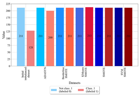
Figure 7.
The number of samples per class for class_1 balanced dataset variations.
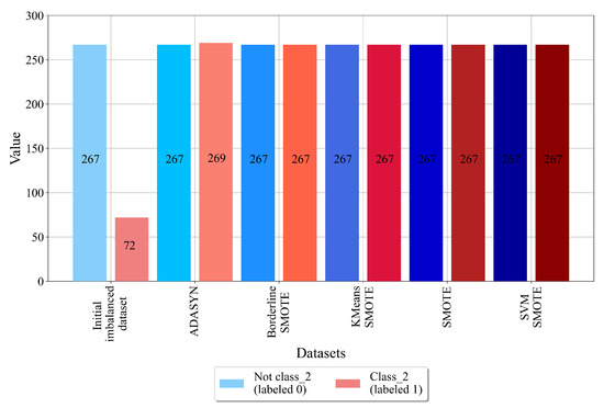
Figure 8.
The number of samples per class for class_2 balanced dataset variations.
As seen from Figure 6, the initial dataset with class_0 as the target variable has 200 samples that do not belong to class_0 and are labeled with 0, and the samples that belong to class_0 are labeled as 1. The idea of using different oversampling techniques is to synthetically increase the number of class_0 samples to achieve the same number of non-class_0 samples. From Figure 6, it can be noted that all oversampling techniques were successfully applied, i.e., balanced dataset variations were achieved. However, the ADASYN technique has a slight imbalance. In this case, the class_0 samples were synthetically increased from 139 up to 187; however, 200 samples were not achieved. Although the dataset is imbalanced, the difference between the number of class samples is smaller. So, this balanced dataset variation can still be used in the GPSC to obtain MEs.
The results of the application of balancing techniques for class_1 are shown in Figure 7.
The initial dataset where the target variable is 1 consists of 211 not-class_1 samples that are labeled as 0 and 128 class_1 samples that are labeled as 1. Using BorderlineSMOTE, SOTE, and SVMSMOTE, a balance between these two classes was achieved. In the case of ADASYN, class_1 was oversampled; however, an equal number of samples was not achieved, i.e., class_1 contains 200 samples. Although this balanced dataset variation is not successfully balanced, it can still be used in the GPSC to obtain MEs. In the case of the KMeansSMOTE technique, class_1 contains 213 samples, which is a slightly higher number of samples than for non-class_1 samples. The results of the application of various oversampling techniques on the dataset with class_2 as the target variable are shown in Figure 8.
In this case, as seen from Figure 8, the target class_2 consists of two classes, i.e., class_2 (labeled as 1) with 72 samples and non-class_2 (labeled as 0) with 267 samples. From the initial values of both classes, it can be noted that this dataset will be challenging to oversample. However, the results showed that all oversampling techniques successfully achieved a balance between class samples and thus created balanced dataset variations.
2.4. Genetic Programming Symbolic Classifier with the Random Hyperparameter Value Search Method
The genetic programming symbolic classifier (GPSC) begins its execution with the development of the initial population (PopSize) of mathematical expressions (MEs). This population is created using the ramped half-and-half method with a random selection of mathematical functions, variables, and constants. All these elements are stored in the primitive set, and the primitive set can be divided into terminals (input variables and constants) and mathematical functions [23]. In this paper, the following mathematical functions were used, i.e., +, −, *, /, , , log, , , , sin, cos, and tan. However, some mathematical functions had to be modified to avoid errors in GPSC execution, and these functions are /, , log, , and . The modified versions of these functions are given in Appendix A.
Before explaining the ramped half-and-half function, it should be noted that the population members inside the GPSC are represented as tree structures. An example of the population member in a tree structure form is shown in Figure 9.
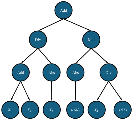
Figure 9.
An example of a population member represented as a tree structure.
The population member shown in Figure 9 has two key components, i.e., nodes and leaves. The nodes contain mathematical functions only, while leaves contain variables and constants. The depth of the syntax tree is one of the measures that is used to measure the size of each population member. The other measurement is the length when the population member is represented in equation format. The depth is generally measured as the number of nodes on the longest path from the root node up to the leaf node. In Figure 9, the root node is the Add function and the depth here is 0. Since all the leaf nodes end on the same level, it does not matter which path is taken to reach the leaf node. So, by counting the nodes, regardless of the path taken, the leaf nodes have a depth of 3. In this case, the depth of the population member is 3.
As previously stated, besides the depth measure, there is the length measure. It should be noted that the GP used in this research displays the best population member (after the GPSC is executed) in functional notation. The length in this notation is measured by counting the number of elements (mathematical functions, variables, and constant values) in the functional form notation. For example, the functional form of the population member shown in Figure 9 can be written as:
where add, mul, div, and abs stand for the mathematical functions of addition, multiplication, division, and absolute value. The length of Equation (2) can be obtained by counting the number of mathematical functions, variables, and constants. So, Equation (2)’s length is 13, i.e., it consists of 13 elements (7 mathematical functions, 4 variables, and 2 constant values).
The ramped half-and-half method combines the full and grow methods equally to create an initial population. In the full method, only mathematical elements are chosen until the max depth is reached; thereafter, only terminals are selected. In the grow method, node elements are randomly chosen from the full primitive set until the max depth is reached; then, only terminals are chosen. To enhance the diversity, population member depths are defined within a range (e.g., the InitDepth hyperparameter ranges from 3 to 18). After population creation, evaluation on the training dataset is conducted using the binary cross-entropy loss fitness function in the GPSC. This value is obtained for each population member in several steps:
- 1.
- First, the output of population members is obtained for all training dataset samples;
- 2.
- This output is used in the Sigmoid function, which can be written in the following form:
- 3.
- Finally, the binary cross entropy loss is obtained using the following equation:
After determining the quality of the population members, the tournament selection (TS) process selects winners for genetic operations (crossover and mutation) based on a defined TS hyperparameter value. TS randomly selects individuals from the population, compares their fitness values, and selects the one with the lowest fitness as the winner.
In the GPSC, four genetic operations are used: crossover and three types of mutation (subtree, point, and hoist mutation). Crossover requires two TS winners; a random subtree from one winner replaces a randomly chosen subtree from the other to create a new member. All mutation operations require only one TS winner. Subtree mutation replaces a randomly chosen subtree with a new one generated from the primitive set. Hoist mutation replaces a subtree with a randomly selected node. Point mutation selects random nodes and replaces them with other constants, variables, or functions with the same arity.
For training, the majority of the training set (typically 99% or more) is used to train population members. A small portion is reserved for the evaluating generation-to-generation fitness and calculating the raw or out-of-bag fitness. This helps ensure consistency between the best fitness and out-of-bag fitness, which can impact the classification performance. The training set size is defined by the maxSamples hyperparameter.
The GPSC, like other GP implementations, faces the bloat problem, where large population members slow down execution or cause memory overflow. To address this, the parsimony pressure method penalizes large population members by increasing their fitness value during TS. Balancing the parsimony coefficient is crucial; a too large value can hinder evaluation, while a too small value can exacerbate bloating.
Two termination criteria exist in the GPSC: the stopping criterion and MaxGen (maximum generations). If either is met, execution halts. Stopping criteria are rarely achieved due to the low predefined fitness thresholds; thus, the execution typically ends when reaching the maximum generation limit.
Given the numerous GPSC hyperparameters, a random hyperparameter value search method was introduced to find the optimal combination. This approach selects values randomly from predefined ranges before each execution. The basic process of defining the RHVS method consists of several steps, i.e.,
- 1.
- Define the initial ranges (lower and upper boundaries) of each GPSC hyperparameter;
- 2.
- Test the GPSC algorithm with each of the boundaries;
- 3.
- If needed due to GPSC execution failure, large MEs, or prolonged execution times, adjust the GPSC hyperparameter values.
The GPSC hyperparameter value ranges used in the RHVS method are listed in Table 4.
Table 4.
The lower and upper boundary of each GPSC hyperparameter value used in the RHVS method.
It should be noted that the sum of all genetic operations must be equal to 1 or slightly less than 1. Otherwise, some TS winners will enter the next generation unchanged. As seen from Table 4, the SubtreeMute range was very narrow (0.95–1), and compared to other genetic operations, its value is very high. An investigation showed that SubtreeMute greatly influences the evolution process, and this is the reason why its value is so high.
2.5. Evaluation Metrics
To evaluate the obtained MEs in this research, several evaluation metrics were used, i.e., accuracy (ACC), the area under receiver operating characteristics curve (AUC), precision, recall, F1-score, and, finally, the confusion matrix. In the context of binary classification, there are terms that describe the outcomes of the classification mode such as true positives (TPs), true negatives (TNs), false positives (FPs), and false negatives (FNs).
- TP—This term occurs when the model correctly predicts the positive class. For example, in medical tests for a disease, a TP means that a model correctly identifies a patient as having the disease;
- TN—This term occurs when the model correctly predicts the negative class. For example, in a medical test for a disease, a TN means the model correctly identifies a patient as not having the disease.
- FP—This term occurs when the model incorrectly predicts the positive class for a sample that is actually negative. In a medical test, an FP means the model incorrectly identifies a healthy patient as having the disease.
- FN—This term occurs when the model incorrectly predicts the negative class for an instance that is actually positive. In a medical test, an FN means the model incorrectly identifies a diseased patient as healthy.
ACC is an evaluation metric that measures the proportion of correct predictions (both TPs and TNs) out of the total number of predictions [24]. This is one of the most commonly used metrics and can be misleading if the classes in the dataset are imbalanced. ACC is calculated using an expression which can be written in the following form:
The AUC is an evaluation metric that is the result of numerical integration of the area below the receiver operating characteristic curve (ROC) [25]. The ROC curve is a graphical plot that illustrates the diagnostic of a binary classifier system, as its discrimination threshold is varied. The AUC quantifies the overall ability of the model to discriminate between positive and negative classes. The range of the AUC is between 0 and 1, where an AUC of 0.5 suggests no discrimination (equal to random guessing) and closer to 1 indicates a good model. The precision score or positive predictive value measures the proportion of TP predictions out of all positive predictions. Basically, the precision score provides the answer to the following question: “of all the positive predictions, how many are actually positive?” [26]. The precision score is calculated using an expression which can be written in the following form:
High values of the precision score indicate a low number of FP errors.
Recall, which is also known as sensitivity or the true positive rate, is an evaluation metric that measures the proportion of actual positives that are correctly identified [26]. The recall score gives the answer to the following question: “out of all the actual positives, how many did we correctly predict as positive?” The recall score is calculated using an expression which can be written in the following form:
A high recall indicates a low number of FN errors.
The F1-score [26] is an evaluation metric used to evaluate the performance of a binary classification model. It is a useful tool when the dataset is imbalanced, which means one class has a higher number of samples than the other. The F1-score is the harmonic mean of precision and recall, combining both metrics into a single value that balances the trade-off between them. The F1-score is calculated using the following expression:
The confusion matrix [27] is a table used to describe the performance of a classification model on a set of data for which the true values are known. The confusion matrix shows the counts of actual values versus predicted classifications made by the classification model and helps to visualize the performance of an algorithm. The basic structure of a confusion matrix is shown in Table 5.
Table 5.
Confusion matrix.
2.6. Train–Test Procedure
A graphical presentation of the train–test procedure is shown in Figure 10.
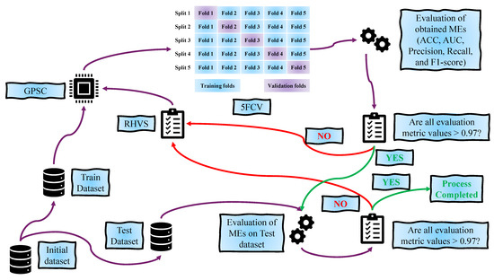
Figure 10.
The graphical representation of train–test procedure used in this research.
As seen from Figure 10 the train test procedure of any balanced dataset variation consists, as in [28], of the following steps:
- 1.
- The balanced dataset variation is divided in a 70:30 ratio into training and test datasets, respectively.
- 2.
- The training dataset is fed into the GPSC; however, before GPSC execution, the RHVS method randomly selects GPSC hyperparameters from a predefined range. Then, the process of GPSC training begins with the 5FCV method. During the training process, evaluation metrics are used to determine the classification performance of obtained MESs on the training and validation folds.
- 3.
- After the training process, the mean and standard deviation of the evaluation metric values obtained on training and validation folds are calculated. If the mean evaluation metric values are higher than 0.9, the process proceeds to the testing phase. Otherwise, the process starts from the beginning with a random selection of GPSC hyperparameter values using the RHVS method.
- 4.
- In the testing phase, the test dataset is provided to 5MEs that passed the training phase to determine the classification performance of these 5MEs on the test dataset. In this phase, the evaluation metric values are obtained.
- 5.
- If all evaluation metric values are higher than 0.9, then the train–test procedure is completed, and this is the best set of MEs obtained for the current balanced dataset variation. On the other hand, if all evaluation metric values are lower than 0.9, the process starts from the beginning with a random selection of hyperparameter values using the RHVS method.
2.7. Threshold-Based Voting Ensemble
As stated in the introduction section, the best MEs obtained with the GPSC on balanced dataset variations will be combined together in a threshold-based voting ensemble to see if the classification performance can be increased. The threshold-based voting ensemble is a method where the decision for a given sample is based on whether the number of classifiers that predict a certain class meets or exceeds a specified threshold. This ensemble is the extension of majority voting, which is the most common form of ensemble decision-making. In majority voting, a class is assigned to a sample if more than half of the classifiers agree on that class. Threshold-based voting generalizes this by allowing the user to set a specific threshold, which could be different from a simple majority.
A predefined number/percentage of classifiers must agree on a particular prediction for it to be selected as the final decision for a sample. This threshold can be tuned based on the problem, dataset, or performance requirements. Unlike majority voting, where the threshold is implicitly 50% plus one vote, threshold-based voting allows for different levels of strictness. In the case of threshold-voting, for example, a threshold of 70% means that at least 70% of the classifiers need to agree on the same prediction for it to be accepted. So, the idea in this paper behind threshold voting is to investigate the influence of a minimum number of correct predictions per dataset sample and to see what the minimum number of correct ME predictions can achieve the highest classification performance, i.e., the highest values of ACC, AUC, and precision, recall, and F1-score.
3. Results
In this section, the results of the conducted research are presented. First, the classification performance of the best MEs is presented, which was obtained using the GPSC on balanced dataset variations. For the best MEs, the optimal combination of GPSC hyperparameter values is also presented, which was obtained using the RHVS method. Then, these best MEs are combined in different variations of ensembles to see if the classification performance can be increased. These ensembles are evaluated on the initial imbalanced dataset.
3.1. The Best MEs Achieved on Balanced Dataset Variations
The best MEs were obtained on each balanced dataset variation using the GPSC with the RHVS method trained with 5FCV. An RHVS was used to find the optimal combination of GPSC hyperparameter values for which the highest classification performance of MEs was achieved. Since training was conducted using 5FCV, the total number of MEs per GPSC execution was 5. Here, the optimal combinations of hyperparameter values using an RHVS for each class obtained for each dataset variation are presented in Table 6, Table 7 and Table 8. Then, the classification performance for each class is graphically presented.
Table 6.
Optimal combinations of GPSC hyperparameters selected with the RVHS method for which the highest classification performance was achieved with the set of MEs on each balanced dataset variation for class_0.
Table 7.
Optimal combinations of GPSC hyperparameters selected with the RVHS method, from which the highest classification performance was achieved with the set of MEs on each balanced dataset variation for class_1.
Table 8.
Optimal combinations of GPSC hyperparameters selected with the RVHS method, from which the highest classification performance was achieved with the set of MEs on each balanced dataset variation for class_2.
From Table 6, PopSize was the largest in the case of the SMOTE dataset and lowest in the case of ADASYN. The largest number of generations was used in the case of KMeansSMOTE, while the lowest was used in the case of SVMMSOTE. The TS was highest in the case of BorderlineSMOTE (391), while the lowest was sued in the case of ADASYN (110). The largest initial tree depth was used in the case of KMeansSMOTE, while the lowest was in the case of BorderlineSMOTE. SubtreeMute, as expected, was the dominant genetic operation. The stopping criteria were never met; i.e., the GPSC was terminated after a maximum number of generations was reached. maxSamples was the highest in the case of ADASYN and the lowest in the case of SVMSMOTE. The parsimony coefficient was the lowest in the case of ADASYN, while in the other cases in Table 6, it is slightly higher but still small. In Table 7, the optimal GPSC hyperparameter values obtained using the RHVS method are listed.
From Table 7, similar trends to those in the previous table can be noted. The largest population was used in the case of SMOTE, the largest NumGen was used in the case of SVMSOTE, the largest TS was used in the case of SMOTE, the largest init depth was used in case of SMOTE, and the stopping criterion was, in all cases, extremely small. The size of the parsimony coefficient was slightly higher than the stopping criterion, but still small. In Table 8, the RHVS optimal hyperparameter combinations are listed.
From Table 8, the largest population was used in the case of the ADASYN dataset, while the smallest was in the case of KMeansSMOTE. MaxGen was the largest in the case of KMeansSMOTE, while it was smallest in the case of SMOTE. The largest TS was used in the case of ADASYN, ensuring a larger diversity in the TS process, while the smallest was in the case of BorderlineSMOTE. The largest InitDepth range was used in the case of ADASYN, while the smallest was in the case of BorderlineSMOTE. SubtreeMute was very large in all cases, as expected. The StoppingCrit value was never reached in any case, so again, all GPSC executions were terminated when the maximum number of generations was reached. The classification performance of the obtained MEs for each class on each balanced dataset variation is shown in Figure 11.
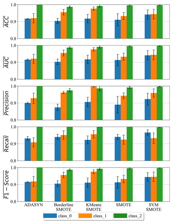
Figure 11.
Classification performance of the best MEs obtained for each class on every balanced dataset variation.
As seen from Figure 11, the MEs obtained for the detection of class_0 have a low classification performance regardless of the balanced dataset variation on which they were trained. However, the highest classification performance was obtained in the case of MEs for the detection of class_2. Higher values of standard deviation in the majority of cases (error bars) can be noted in the case of class_1 MEs. A variable standard deviation can be noted in the case of MEs for class_0. For example, the lowest standard deviation of MEs for class_0 can be noted in the case of a dataset balanced with the ADASYN technique. The highest standard deviation value for MEs of class_0 can be noted in the case of the dataset balanced with the SMOTE technique.
3.2. Threshold-Voting Ensemble
After the best MEs were obtained on each balanced dataset variation, they were grouped together in an ensemble and tested on the initial imbalanced dataset. The idea of this ensemble is to find the minimum number of accurate predictions of MEs per dataset sample, i.e., the threshold value. Besides the threshold value with the highest classification performance in this investigation, the threshold range in which the classification performance is high was determined. The classification performance of threshold voting ensembles for each class is shown in Figure 12.
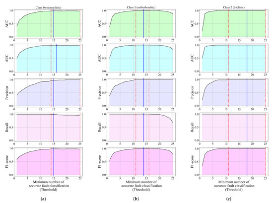
Figure 12.
The classification performance of threshold-based voting ensembles for each class versus the minimum number of accurate fault classifications per sample (threshold). (a) Classification performance of threshold-based voting ensembles for class_0 (monoclinic), (b) Classification performance of threshold-based voting ensembles for class_1 (orthorhombic), and (c) Classification performance of threshold-based voting ensembles for class_2 (triclinic).
For class_0, if the threshold value is equal to 1, all evaluation metric values, with recall as an exception, are low. As the threshold increases, the classification performance also increases. The threshold voting ensemble for the detection of class_0 achieved the highest classification performance when the threshold value was 15 (, , , , and ). However, this ensemble achieves the highest classification performance (all evaluation metrics values are higher than 0.97) when the threshold value is in the 14 to 25 range. However, only the recall value decreases from the initial 0.99281 at threshold 14 to 0.94245 at threshold 25. The confusion matrices for thresholds 14, 15, and 25 are shown in Figure 13.
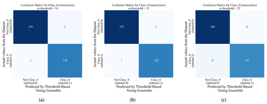
Figure 13.
The classification matrices for thresholds 14, 15, and 25. (a) Classification matrix for the threshold-based voting ensemble for class_0 with the threshold set to 14, (b) Classification matrix for the threshold-based voting ensemble for class_0 with the threshold set to 15, and (c) Classification matrix for threshold-based voting ensemble for class_0 with threshold set to 25.
As seen from Figure 13, the highest classification performance is validated in the form of the confusion matrix for 15 threshold values. In this case, the class_0 (labeled 1) threshold-based voting ensemble correctly predicted 138 out of 139 samples and one sample was misclassified. Regarding the samples that do not belong to class_0, 197 samples were correctly classified, while 3 were misclassified. The other two cases, threshold 14 and threshold 25, showed slightly lower classification performances; i.e., in the case of threshold 14, one class_0 sample and five non-class_0 samples were misclassified, and in the case of threshold 25, a total of eight class_0 samples were misclassified.
In the case of class_1, all evaluation metric values are the lowest when the threshold is equal to 1, with recall as an exception, which has the highest possible value. When increasing the threshold value, the classification performance also increases. The highest classification performance (all evaluation metric values are equal to 1) was achieved when the threshold value was in the 11 to 16 range. The blue line in Figure 12b is just one threshold value (14) randomly chosen from the 11 to 16 range, since all evaluation metric values were the highest possible. As the threshold value increases beyond 16, the ACC, AUC, recall, and F1-score values tend to decrease while the precision score value remains constant and equal to 1. Since the highest classification performance was achieved for thresholds in the 11 to 16 range, the confusion matrix for a randomly chosen value of 14 is shown in Figure 14.
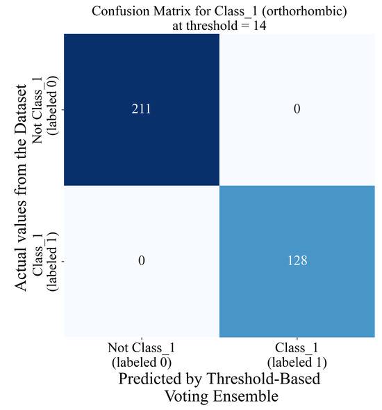
Figure 14.
The classification matrix of the threshold-based voting ensemble for a threshold value of 14.
As seen from Figure 14, the threshold-based voting ensemble for a threshold value of 14 showed an excellent classification performance; i.e., all the samples from the class_1 imbalanced dataset were correctly classified.
The lowest classification performance for threshold voting ensembles in the case of class_2 (Figure 12c) was noted when the threshold value is equal to 1. As the threshold value increases, the classification performance increases rapidly, and when the threshold value reaches 11, all evaluation metric values are equal to 1. So, for the 11 to 25 threshold range (indicated with red dashed lines in Figure 12c), all evaluation metric values are perfect. The blue line in this case represents a randomly chosen threshold value (18) in the threshold range where the evaluation metric values are all perfect. The confusion matrix for the threshold-based voting ensemble with a threshold value of 18 is shown in Figure 15.
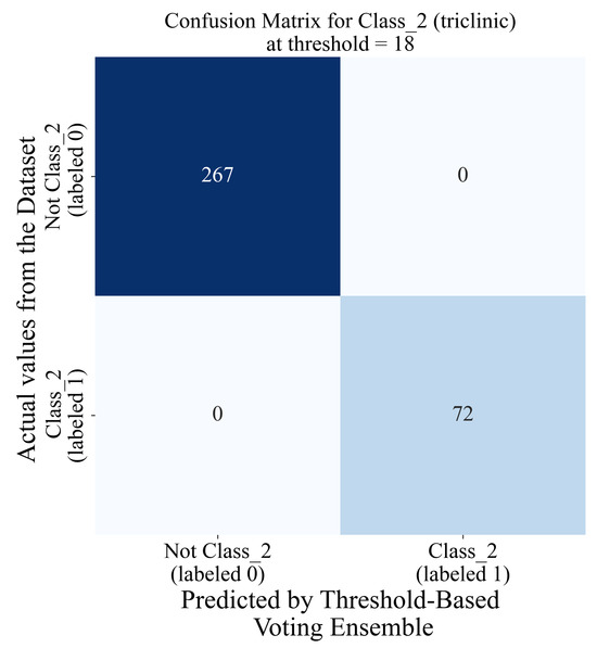
Figure 15.
The classification matrix for the threshold-based voting ensemble for class_2 and a threshold value of 18.
From Figure 15, the same trend as in the case of the threshold-based voting ensemble for class_1 can be observed, i.e., perfect classification of the data samples of the initial class_1 imbalanced dataset variation. The best classification performances of threshold-based voting ensembles for class_0, 1, and 2 are summarized in Table 9.
Table 9.
The highest classification performance of threshold-based voting ensembles for each class, evaluated on initial imbalanced dataset variations.
From Table 9, the threshold-based classification performance is perfect for classes 1 and 2, while it is slightly lower for class_0, which indicates that by using GPSC MEs in threshold-based voting ensembles and adjusting the threshold, a high classification performance can be obtained.
4. Discussion
The publicly available dataset used in this research required some preprocessing, i.e., transformations of original Formula, Spacegroup, Had Bandstructure, and target variable (Crystal System) values to strings. The first variable, Material ID, was removed from the initial variables since it had no relevant value to the dataset. The formula values were simply transformed using the label encoder from strings to integers. This is not quite the right approach but due to the limited number of chemical compounds used in crystal systems, the approach can be slightly justified.
The initial statistics revealed that all dataset variables have the same number of samples; i.e., there are no missing samples. An investigation showed that the multiclass target variable is imbalanced. Since the GPSC cannot be used in multiclass problems, three different imbalanced variations were created from the original dataset (for class_0, class_1, and class_2). When this was completed, different dataset oversampling techniques were used to see if balanced dataset variations could be obtained. In reality, all the oversampling techniques were successful in achieving a balance between classes and thus created balanced dataset variations, with the exception of ADAYN. This method, for all three classes, did achieve some oversampling; however, in the end, the majority class did not have the same or had a slightly lower/higher number of samples. However, this imbalance did have some effect, since the MEs for class_0 and 1 obtained on this balanced dataset variation have a slightly lower classification performance.
The best MEs obtained on balanced dataset variations for class_0 have a consistently low classification performance when compared with the best MEs for other classes (Figure 11). The standard deviation for the best MEs for class zero obtained on the ADASYN-balanced dataset variation was the smallest, while the largest standard deviation was noted in the case of the SMOTE-balanced dataset variation. The best MEs for class_1 have a higher classification performance with a higher variability (Figure 11). The highest classification performance can be noted in the case of the KMeansSMOTE-balanced dataset variation, while the smallest was observed in the case of the ADASYN-balanced dataset variation. In the case of class_2, the best MEs achieved the highest classification performance with accuracy values near or equal to 1.0.
Regarding the GPSC hyperparameter values, it was found that subtree mutation initially had a great influence on the evolution process, so its value was very high when compared to other genetic operations. The low stopping criterion (fitness function value) was never met by any population member, so GPSC execution ended after the maximum number of generations was reached in every investigation conducted in this research. The problem is that it took a long time to obtain the best MEs for each balanced dataset variation. Although the parsimony coefficient was low in every investigation, the population members during each GPSC execution did grow but it did not lead to the bloating phenomenon.
The initial idea of combining the best MEs into a threshold-based voting ensemble was to see if the classification performance could be increased by adjusting the threshold value. The threshold value is the minimum number of correct predictions by MEs per sample. For each class, there were a total of five balanced dataset variations and on each dataset, a total of five best MEs were obtained due to the 5FCV training process. So, for each class, the threshold-based voting ensemble will consist of 25 MEs and the goal is to find the threshold range or value for which the classification performance is the highest. This was particularly interesting for class_0, since the best MEs obtained on balanced dataset variations achieved an accuracy within a range of 0.9–0.92. The threshold-based voting ensemble for class_0 showed that if the threshold range is 14 to 25, the classification performance, i.e., the values of ACC, AUC, precision, recall and F1-score, is around 0.98. This is a huge improvement when compared to the classification performance achieved with the best MEs obtained on balanced dataset variations. The threshold-based voting ensemble for class_1 and class_2 achieved a perfect classification performance if the threshold values were in the 11–16 and 11–25 ranges, respectively. This is a great improvement for class_1 when the classification performance is compared to the best MEs obtained on the balanced dataset variation. The best MEs for class_2 had already achieved a high classification performance on balanced dataset variations, so this was just minor improvement.
In Table 10, the accuracy values obtained in this research are compared to the results achieved in other research papers.
Table 10.
A summary of the literature.
When the results from Table 10 are compared, it can be noted that the results obtained in this paper with the proposed research methodology outperform the results from other research papers. The benefit of using the proposed research methodology is that the MEs are obtained with a high classification accuracy. They are easier to store and reuse than other ML-trained models.
5. Conclusions
In this paper, a publicly available dataset was used in a GPSC to obtain MEs that could be used for the detection of the crystal structure of Li-ion batteries. The initial problem with the dataset is that the target variable contained three classes; i.e., it was initially a multiclass problem. However, the target variable was divided into three separate variables using the one-versus-rest approach, and by doing so, datasets for the detection of class_0, 1, and 2 were created. An additional problem with these datasets is that they were imbalanced, so different balancing techniques (ADASYN, BorderlineSMOTE, KMeansSMOTE, SMOTE, and SVMSMOTE) were used to achieve a balance between class samples. These balanced dataset variations were used in the GPSC to obtain MEs. Since the GPSC has a large number of hyperparameters, the RHVS method was applied to search for the optimal combination of GPSC hyperparameters to obtain MEs with a high classification performance. The GPSC training process was conducted using 5FCV, and using this training process, a total of five MEs were obtained and thus a robust solution was generated. After the GPSC was trained on all balanced dataset variations, the best sets of MEs were extracted for each class to combine them in a threshold-based voting ensemble. The idea of a threshold-based voting ensemble is to find the threshold for which the ensemble of MEs for each class has the highest classification performance. The analysis showed that the ensemble of MEs for each class has its own threshold range for the highest classification performance (area surrounded by the red dashed lines). Using the approach proposed in this investigation showed that a balanced dataset has a great influence on the classification performance.
Based on the conducted investigation, the following conclusions can be drawn:
- MEs that detect the crystal system type in Li-ion batteries with a high classification performance can be obtained using the GPSC.
- Oversampling techniques were very useful in achieving balanced dataset variations, and by using these in the GPSC, the GPSC produced MEs with a high classification performance.
- The RHVS method has been successfully developed and applied. This method found the optimal combination of GPSC hyperparameters for each balanced dataset variation, which were used to achieve the highest classification performance.
- The application of the 5FCV training process in this paper generated five MEs per GPSC execution. A large number of MEs per execution could suggest a robust classification performance.
- The best MEs obtained with GPSC + 5FCV + RHVS were combined together and used in a threshold-based ensemble. The application of the threshold improved the classification performance. This is especially true for class_0, which had the lowest classification performance when compared to the other two classification performances obtained with the GSPC on the balanced dataset variations.
As with any other research, this study also has its pros and cons. The pros of this research are as follows:
- Unlike any other research paper, the GPSC can produce MEs that are simple and easily stored and reused.
- All the oversampling techniques used in this research are fast and do not require additional fine-tuning of their parameters, since the majority of them with default parameters produce balanced dataset variations.
- The GPSC + RVHS + 5FCV is a powerful tool that generated a set of the best MEs per balanced dataset variation with a high classification performance.
- The threshold-based voting ensemble proved to be another useful tool for improving the classification performance for each class.
The cons of this research are as follows:
- The GPSC execution time is long, which can be attributed to the large population or longer maximum number of generations.
- The ADASYN technique did not achieve a perfect balance with the default parameters. Although the dataset variation obtained with ADASYN was not properly balanced, it was still used in research.
- Although the GPSC + RHVS + 5FCV is a powerful tool to obtain MESs with a high classification performance, a problem remains regarding the execution time, since the GPSC can take a long time to execute because the 5FCV process during GPSC training must be repeated five times.
Based on the conducted research, future work will be focused on speeding up the GPSC training process. This can be achieved by further fine-tuning the initial GPSC hyperparameter value ranges. If this time is reduced, the process of training and developing the GPSC research could be improved. Further investigations will involve the fine-tuning of ADAYN hyperparameter values to see if the perfect balance can be achieved.
Author Contributions
Conceptualization, N.A. and S.B.Š.; methodology, N.A.; software, N.A.; validation, N.A. and S.B.Š.; formal analysis, N.A. and S.B.Š.; investigation, N.A. and S.B.Š.; resources, N.A.; data curation, N.A. and S.B.Š.; writing—original draft preparation, N.A. and S.B.Š.; writing—review and editing, N.A. and S.B.Š.; visualization, N.A.; supervision, N.A.; project administration, N.A.; funding acquisition, S.B.Š. All authors have read and agreed to the published version of the manuscript.
Funding
This research was (partly) supported by the CEEPUS network CIII-HR-0108, the Erasmus+ project WICT under Grant 2021-1-HR01-KA220-HED-000031177, and the University of Rijeka Scientific Grant uniri-mladi-technic-22-61.
Institutional Review Board Statement
Not applicable.
Informed Consent Statement
Not applicable.
Data Availability Statement
The dataset is publicly available on Kaggle: https://www.kaggle.com/datasets/divyansh22/crystal-system-properties-for-liion-batteries (accessed on 10 May 2024).
Conflicts of Interest
The authors declare no conflicts of interest.
Appendix A. Modification of Mathematical Functions
As already stated in the description of the GPSC, some mathematical functions had to be modified to avoid early termination of the GPSC due to them not being a number, due to memory overflow or due to them generating imaginary values. These mathematical functions are division, square root, natural logarithm, and logarithm with 2 and 10 bases. The division function will calculate the division if the absolute value of the denominator is greater than 0.001; otherwise, it will return 1. The division function can be written as:
It should be noted that and are two variables that do not have any connection with dataset variables and are defined here for demonstration purposes only. The square root function will determine the absolute value of the argument below the square root before the application of the square root. This function can be written as:
The natural logarithm and logarithm with bases 2 and 10 can be written as:
where i indicates the base of the logarithm (natural, 2, and 10). So, all three logarithms work the same way; i.e., if |x| is greater than 0.001, the function will calculate the logarithm value. Otherwise, it will return 0.
Appendix B. Acquisition of Obtained MEs from this Research
The mathematical equations obtained in this research are available online at https://github.com/nandelic2022/Crystal-Structure-LION.git (accessed on 20 May 2024). After downloading the equations and preparing the Python script for application to new data, make sure that the dataset variables correspond to the dataset variables defined in Table 3. After obtaining the output using these equations, please use the Sigmoid function to determine the class.
References
- Chen, Q.; Zhu, L.; Xia, C.; Xie, L.; Han, Q.; Katiyar, S.; Gomez, J.F.F.; Wu, X.; Yang, L.; Yi, L.; et al. Effect of sodium concentration on the structure and electrochemical properties of NaxMnO2+ z cathode materials. J. Electroanal. Chem. 2024, 956, 118085. [Google Scholar] [CrossRef]
- Zhang, T.; Li, D.; Tao, Z.; Chen, J. Understanding electrode materials of rechargeable lithium batteries via DFT calculations. Prog. Nat. Sci. Mater. Int. 2013, 23, 256–272. [Google Scholar] [CrossRef]
- Cai, Z.; Ji, H.; Ha, Y.; Liu, J.; Kwon, D.H.; Zhang, Y.; Urban, A.; Foley, E.E.; Giovine, R.; Kim, H.; et al. Realizing continuous cation order-to-disorder tuning in a class of high-energy spinel-type Li-ion cathodes. Matter 2021, 4, 3897–3916. [Google Scholar] [CrossRef]
- Yang, J.; Xia, Y. Suppressing the phase transition of the layered Ni-rich oxide cathode during high-voltage cycling by introducing low-content Li2MnO3. ACS Appl. Mater. Interfaces 2016, 8, 1297–1308. [Google Scholar] [CrossRef] [PubMed]
- Deng, D. Li-ion batteries: Basics, progress, and challenges. Energy Sci. Eng. 2015, 3, 385–418. [Google Scholar] [CrossRef]
- Kim, S.; Aykol, M.; Hegde, V.I.; Lu, Z.; Kirklin, S.; Croy, J.R.; Thackeray, M.M.; Wolverton, C. Material design of high-capacity Li-rich layered-oxide electrodes: Li 2 MnO 3 and beyond. Energy Environ. Sci. 2017, 10, 2201–2211. [Google Scholar] [CrossRef]
- Kurzweil, P.; Scheuerpflug, W.; Schell, C.; Schottenbauer, J. Useful Quantities and Diagram Types for Diagnosis and Monitoring of Electrochemical Energy Converters Using Impedance Spectroscopy: State of the Art, Review and Outlook. Batteries 2024, 10, 177. [Google Scholar] [CrossRef]
- Li, J.; Zhang, X.; Lu, Y.; Linghu, K.; Wang, C.; Ma, Z.; He, X. Electrospun fluorinated polyimide/polyvinylidene fluoride composite membranes with high thermal stability for lithium ion battery separator. Adv. Fiber Mater. 2022, 4, 108–118. [Google Scholar] [CrossRef]
- Sekhar, S.C.; Ramulu, B.; Arbaz, S.J.; Nagaraju, M.; Yu, J.S. Cobalt–Nickel Vanadate Nanonest Colonies Deposited Carbon Fabric as a Bifunctional Electrode for Li-Ion Batteries and Oxygen-Evolution Reactions. Adv. Fiber Mater. 2024, 1–12. [Google Scholar] [CrossRef]
- Jia, H.; Dirican, M.; Sun, N.; Chen, C.; Yan, C.; Zhu, P.; Dong, X.; Du, Z.; Cheng, H.; Guo, J.; et al. Advanced ZnSnS3@ rGO Anode Material for Superior Sodium-Ion and Lithium-Ion Storage with Ultralong Cycle Life. ChemElectroChem 2019, 6, 1183–1191. [Google Scholar] [CrossRef]
- Fang, M.; Yue, X.; Dong, Y.; Chen, Y.; Liang, Z. A temperature-dependent solvating electrolyte for wide-temperature and fast-charging lithium metal batteries. Joule 2024, 8, 91–103. [Google Scholar] [CrossRef]
- Xu, X.; Yue, X.; Chen, Y.; Liang, Z. Li Plating Regulation on Fast-Charging Graphite Anodes by a Triglyme-LiNO3 Synergistic Electrolyte Additive. Angew. Chem. Int. Ed. 2023, 62, e202306963. [Google Scholar] [CrossRef] [PubMed]
- Prasshanth, C.; Lakshminarayanan, A.K.; Ramasubramanian, B.; Ramakrishna, S. Progress of machine learning in materials design for Li-Ion battery. Next Mater. 2024, 2, 100145. [Google Scholar]
- Shandiz, M.A.; Gauvin, R. Application of machine learning methods for the prediction of crystal system of cathode materials in lithium-ion batteries. Comput. Mater. Sci. 2016, 117, 270–278. [Google Scholar] [CrossRef]
- Prosini, P.P. Crystal group prediction for lithiated manganese oxides using machine learning. Batteries 2023, 9, 112. [Google Scholar] [CrossRef]
- Yin, Y.; Xu, G.; Xie, Y.; Luo, Y.; Wei, Z.; Li, Z. Utilizing Deep Learning for Crystal System Classification in Lithium-Ion Batteries. J. Theory Pract. Eng. Sci. 2024, 4, 199–206. [Google Scholar] [CrossRef] [PubMed]
- Sedgwick, P. Pearson’s correlation coefficient. BMJ 2012, 345, e4483. [Google Scholar] [CrossRef]
- He, H.; Bai, Y.; Garcia, E.A.; Li, S. ADASYN: Adaptive synthetic sampling approach for imbalanced learning. In Proceedings of the 2008 IEEE International Joint Conference on Neural Networks (IEEE World Congress on Computational Intelligence), Hong Kong, China, 1–8 June 2008; pp. 1322–1328. [Google Scholar]
- Han, H.; Wang, W.Y.; Mao, B.H. Borderline-SMOTE: A new over-sampling method in imbalanced data sets learning. In Proceedings of the International Conference on Intelligent Computing (ICIC), Hefei, China, 23–26 August 2005; pp. 878–887. [Google Scholar]
- Chang, C.C.; Li, Y.Z.; Wu, H.C.; Tseng, M.H. Melanoma detection using XGB classifier combined with feature extraction and K-means SMOTE techniques. Diagnostics 2022, 12, 1747. [Google Scholar] [CrossRef] [PubMed]
- Fernández, A.; Garcia, S.; Herrera, F.; Chawla, N.V. SMOTE for learning from imbalanced data: Progress and challenges, marking the 15-year anniversary. J. Artif. Intell. Res. 2018, 61, 863–905. [Google Scholar] [CrossRef]
- Nithya, R.; Kokilavani, T.; Beena, T.L.A. Balancing cerebrovascular disease data with integrated ensemble learning and SVM-SMOTE. Netw. Model. Anal. Health Inform. Bioinform. 2024, 13, 12. [Google Scholar] [CrossRef]
- Langdon, W.B.; Gustafson, S.M. Genetic programming and evolvable machines: Ten years of reviews. Genet. Program. Evolvable Mach. 2010, 11, 321–338. [Google Scholar] [CrossRef]
- Sokolova, M.; Japkowicz, N.; Szpakowicz, S. Beyond accuracy, F-score and ROC: A family of discriminant measures for performance evaluation. In Proceedings of the 19th Australian Joint Conference on Artificial Intelligence, Hobart, Australia, 4–8 December 2006; pp. 1015–1021. [Google Scholar]
- de Hond, A.A.; Steyerberg, E.W.; van Calster, B. Interpreting area under the receiver operating characteristic curve. Lancet Digit. Health 2022, 4, e853–e855. [Google Scholar] [CrossRef] [PubMed]
- Goutte, C.; Gaussier, E. A probabilistic interpretation of precision, recall and F-score, with implication for evaluation. In Proceedings of the 27th European Conference on IR Research, ECIR 2005, Santiago de Compostela, Spain, 21–23 March 2005; pp. 345–359. [Google Scholar]
- Townsend, J.T. Theoretical analysis of an alphabetic confusion matrix. Percept. Psychophys. 1971, 9, 40–50. [Google Scholar] [CrossRef]
- Anđelić, N.; Baressi Šegota, S. Development of Symbolic Expressions Ensemble for Breast Cancer Type Classification Using Genetic Programming Symbolic Classifier and Decision Tree Classifier. Cancers 2023, 15, 3411. [Google Scholar] [CrossRef] [PubMed]


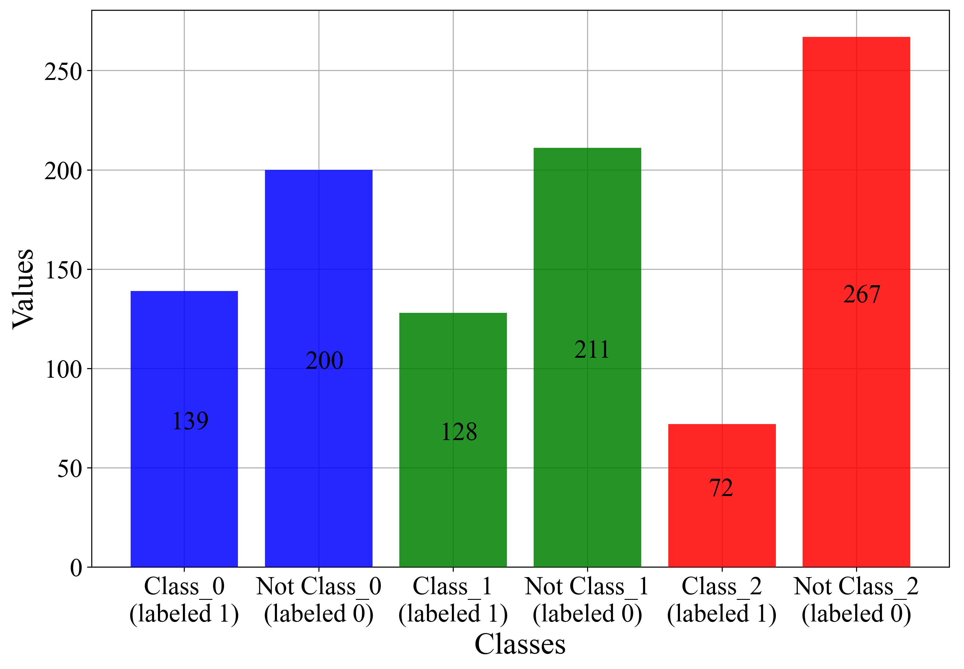

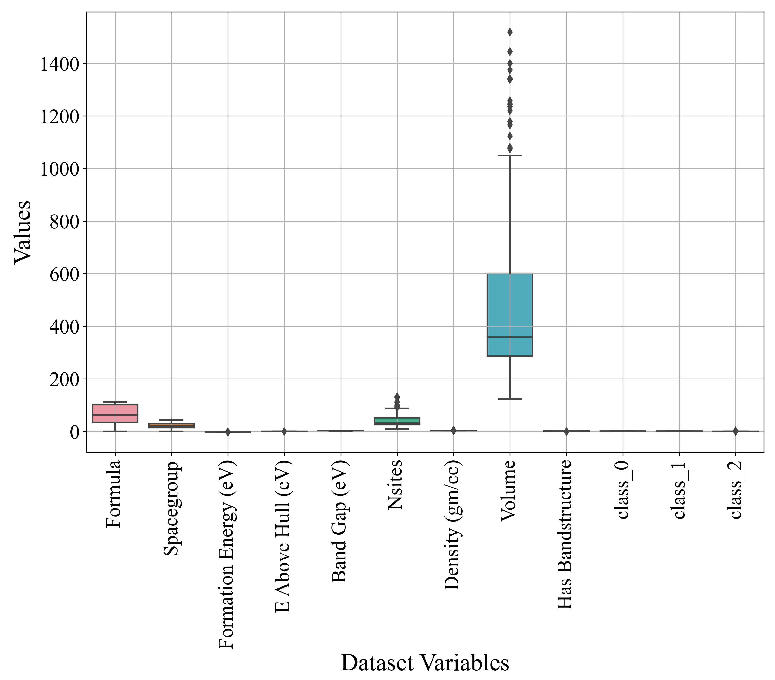
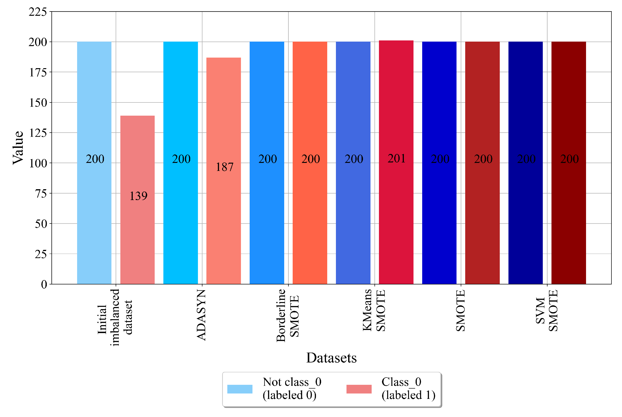

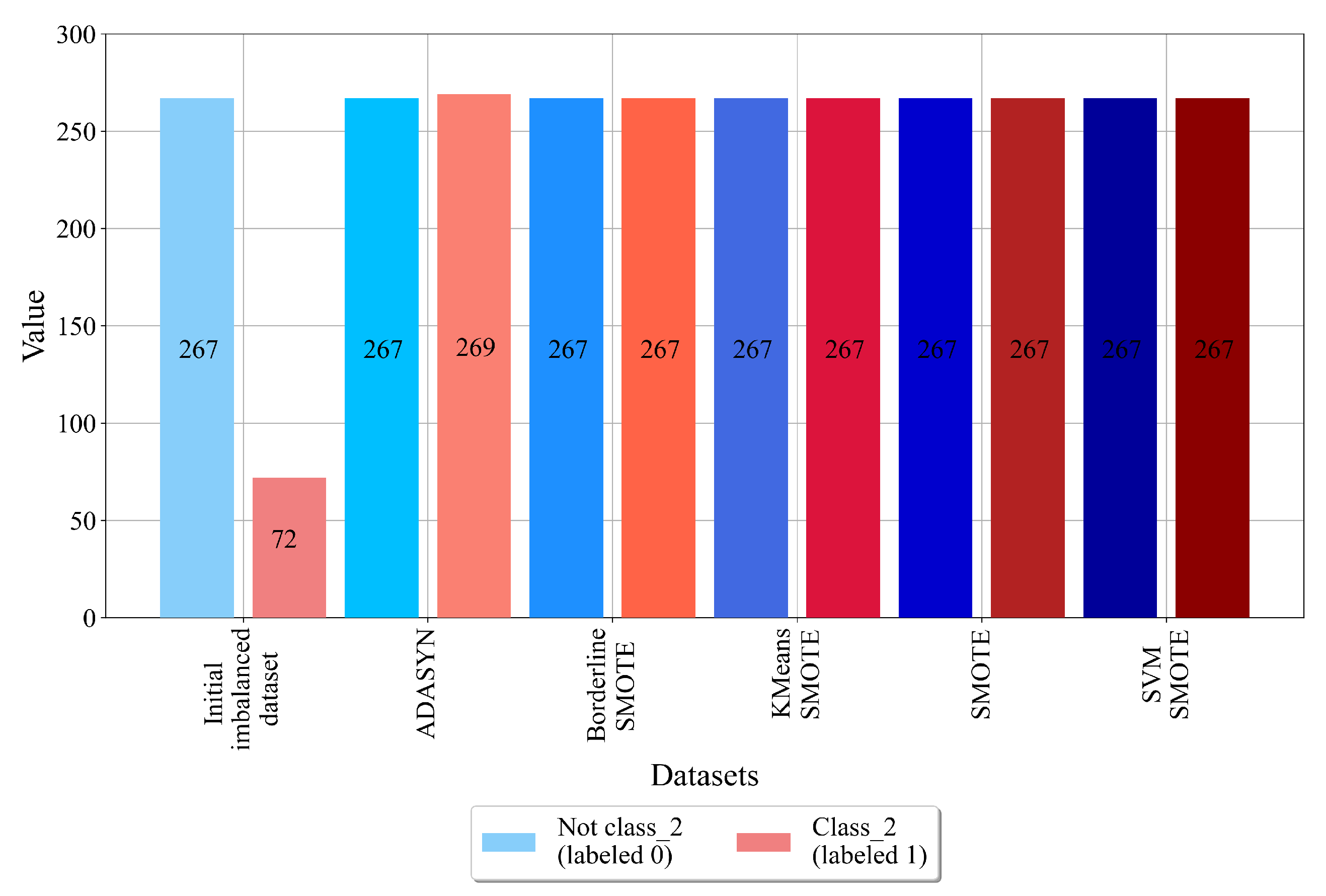
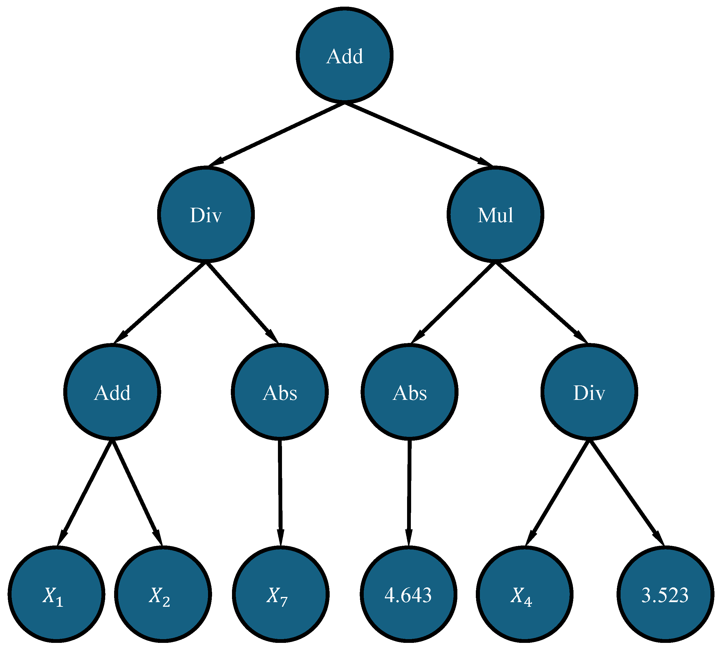

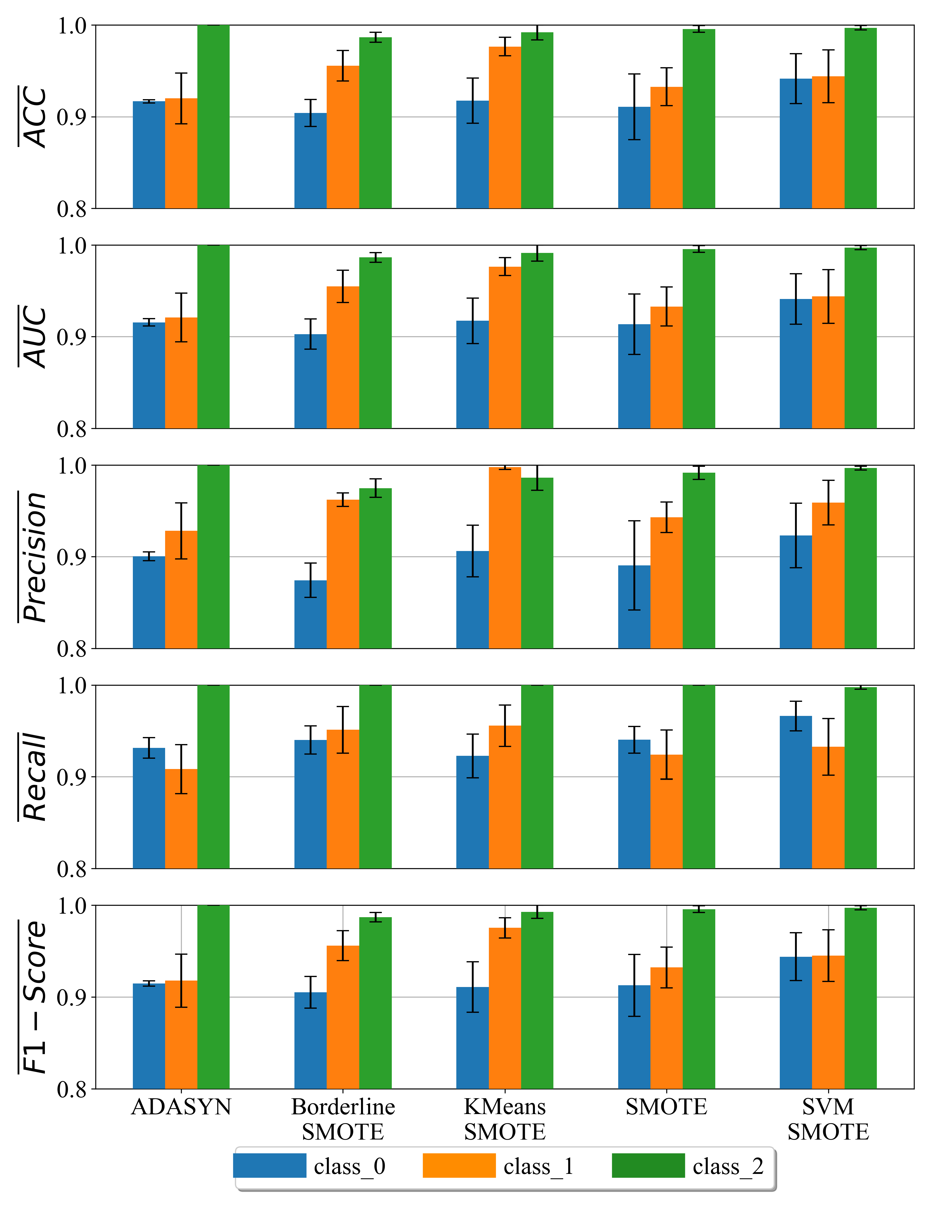
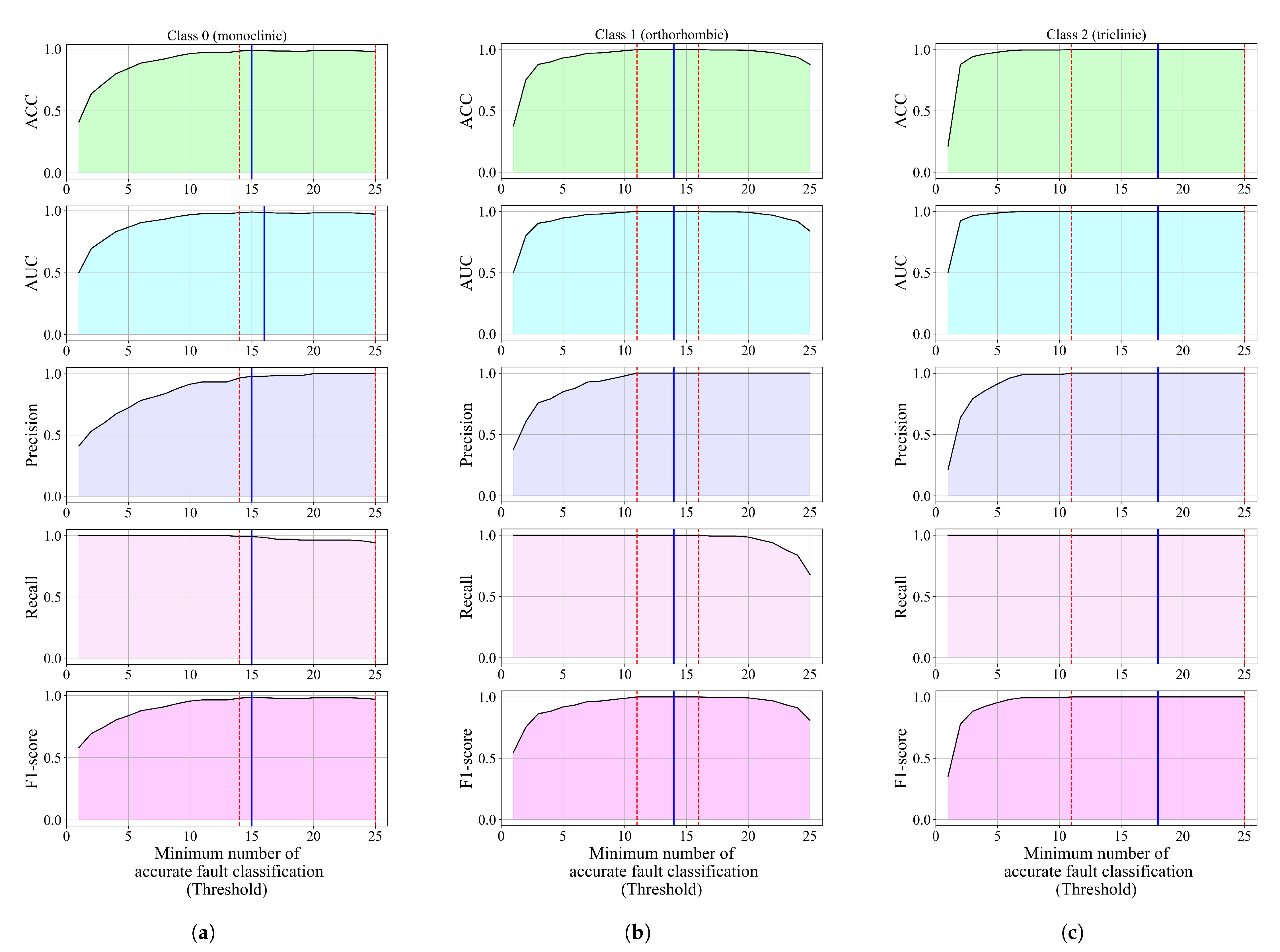
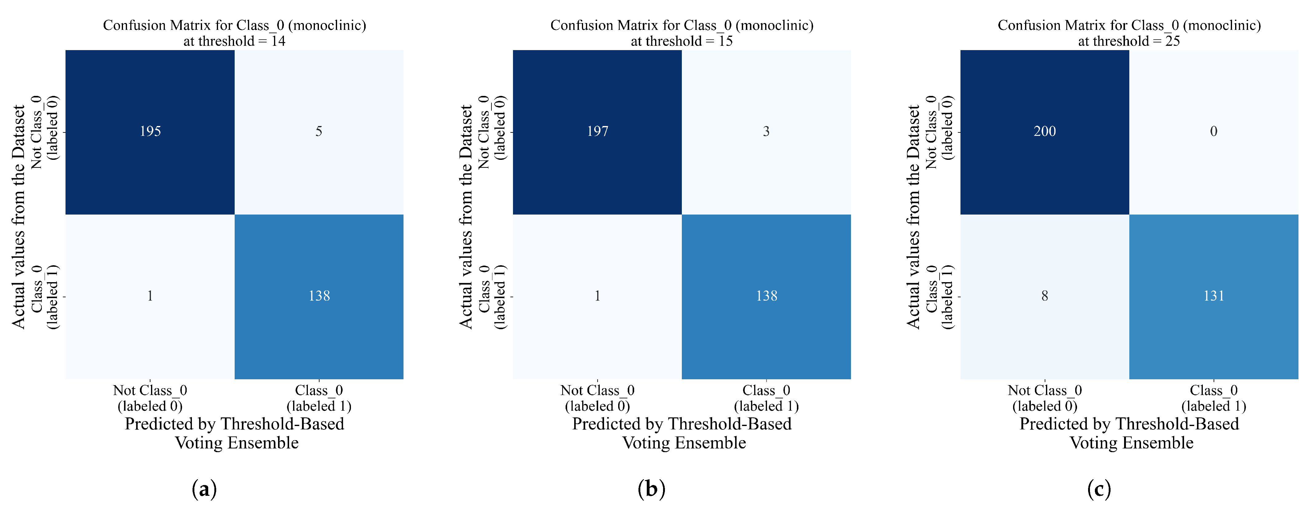


Disclaimer/Publisher’s Note: The statements, opinions and data contained in all publications are solely those of the individual author(s) and contributor(s) and not of MDPI and/or the editor(s). MDPI and/or the editor(s) disclaim responsibility for any injury to people or property resulting from any ideas, methods, instructions or products referred to in the content. |
© 2024 by the authors. Licensee MDPI, Basel, Switzerland. This article is an open access article distributed under the terms and conditions of the Creative Commons Attribution (CC BY) license (https://creativecommons.org/licenses/by/4.0/).