Adaptive Speed Control Scheme Based on Congestion Level and Inter-Vehicle Distance

Abstract

Cellular vehicle-to-everything (C-V2X) enables short-distance communication between vehicles and other users to improve road safety through data sharing. Conventional research on C-V2X typically assumes that vehicles travel at the same speed with a fixed inter-vehicle distance (${Dis}_{inter}$). However, this assumption does not reflect the real driving environment or promote road traffic efficiency. Conversely, assigning different speeds to vehicles without a structured approach inevitably increases the collision risk. Therefore, determining appropriate speeds for each vehicle in the C-V2X framework is crucial. To this end, considering the road environment and mobility, this study introduces an adaptive speed mechanism based on the congestion level of a zone and ${Dis}_{inter}$. First, the given scenario is divided into several zones. Subsequently, based on the congestion level of a zone and the ${Dis}_{inter}$ level, an adaptive speed is defined for each vehicle. This approach ensured that vehicles adopt lower speeds in congested situations to reduce the collision probability and higher speeds in sparse traffic cases to improve traffic efficiency. The performance of the proposed adaptive speed scheme is compared with that of conventional fixed-speed settings. The results show that the adaptive speed control scheme outperforms conventional fixed-speed schemes in terms of the packet reception ratio (PRR) and collision ratio (CR). Specifically, the proposed mechanism can reduce the CR to 0 and ensure that the PRR is higher than 0.98 in low-density scenarios.

1. Introduction

Cellular vehicle-to-everything (C-V2X) supports vehicle-to-vehicle (V2V), vehicle-to-infrastructure (V2I), vehicle-to-network (V2N), and vehicle-to-pedestrian (V2P) communication links [1]. Advances in wireless networks have enabled C-V2X to provide an enhanced quality of service and new radio V2X (NR-V2X) to support broadcast, multicast, and unicast data transmission [2]. The supported packet types are periodic cooperative awareness messages (CAMs) and event-triggered decentralised environmental notification messages (DENMs) [3,4]. In addition to basic safety and entertainment services, NR-V2X also defines four advanced V2X use cases, i.e., extended sensors, advanced driving, remote driving, and vehicle platooning [5]. Extended sensors provide drivers with reliable information regarding the environment by accurately identifying surrounding objects using lidar, radar, and high-definition cameras [6]. Advanced driving and remote driving represent the ultimate goals of V2X development, aiming to promote safe driving [7,8,9]. Platooning allows vehicles to be connected in groups, with the first vehicle in each platoon acting as the leader and the remaining vehicles functioning as members [10]. To maintain the safety distance, vehicles in a platoon are required to share status information, including their speed, direction, and purpose. This setup helps reduce the safe distance and overall fuel consumption and increases road capacity [11].

Vehicle speed considerably affects the distance between vehicles. When the speed of the front vehicle is higher than that of the rear vehicle, the safety distance increases but the road capacity decreases. In contrast, when the vehicle in front moves slower than the vehicle behind, the distance between the two vehicles reduces, which increases the road capacity but also the collision risk. Therefore, configuring reasonable vehicle speeds and safety distances can improve transportation efficiency and ensure road safety. However, the existing research on C-V2X has been limited to scenarios with identical fixed-speed settings for all vehicle users, which neither simulates real vehicle movement nor enhances traffic efficiency. Although there are already systems like adaptive cruise control (ACC) and CACC that help members of a truck platoon adjust speed and maintain distance, these technologies mainly rely on external devices such as cameras and radar, which are greatly affected by environmental changes and light reflections [12]. In addition, because CACC only considers the local situation between vehicles rather than the coordination of the overall and local environments, it cannot guarantee that the traffic efficiency of the overall scenario will be improved while providing a suitable speed [13]. Therefore, a personality-based adaptive vehicle speed scheme for all vehicles in C-V2X communication must be established. Such a mechanism can help increase road capacity, enhance traffic efficiency, reduce the probability of collisions, and improve inter-vehicle communication.

Thus, this study was aimed at clarifying the influence of vehicle speed on traffic efficiency in NR-V2X scenarios where vehicles and infrastructure coexist and identifying strategies to optimise the vehicle speed and inter-vehicle distance (${Dis}_{inter}$), to improve the overall traffic efficiency. First, communication performance under same or different vehicle speed configurations is analysed. Subsequently, an adaptive speed mechanism based on the current environment is established to improve transportation efficiency. This mechanism provides speed recommendations based on the congestion level ($CL$) of the zone and the distance level ($DL$) between a vehicle and its front neighbours. The proposed mechanism adjusts the speed according to the personality of the vehicle, thereby reducing collisions due to small ${Dis}_{inter}$ values, while preventing the decreased road capacity associated with a large ${Dis}_{inter}$. In addition, the algorithm considers the status of each zone to reduce the possibility of vehicle locations overlapping. This can help minimise conflicts in resource selection caused by similar environments and enhance communication. The contributions of this work can be summarised as follows:

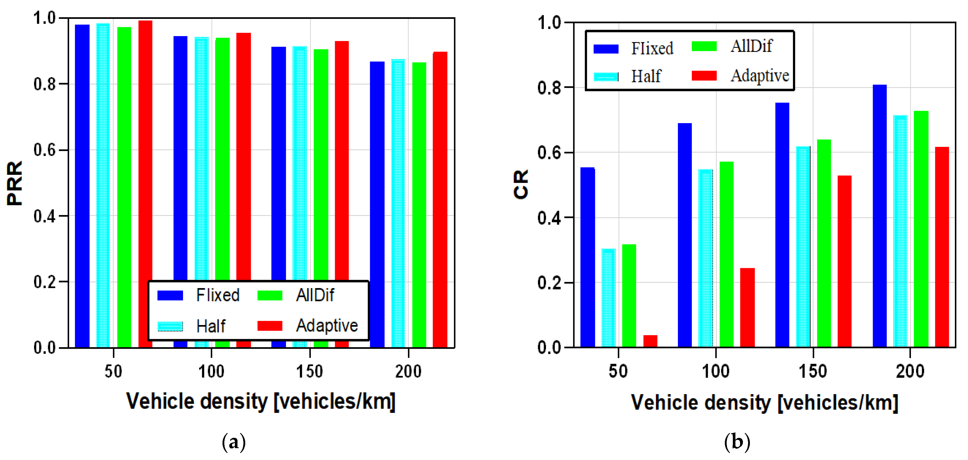
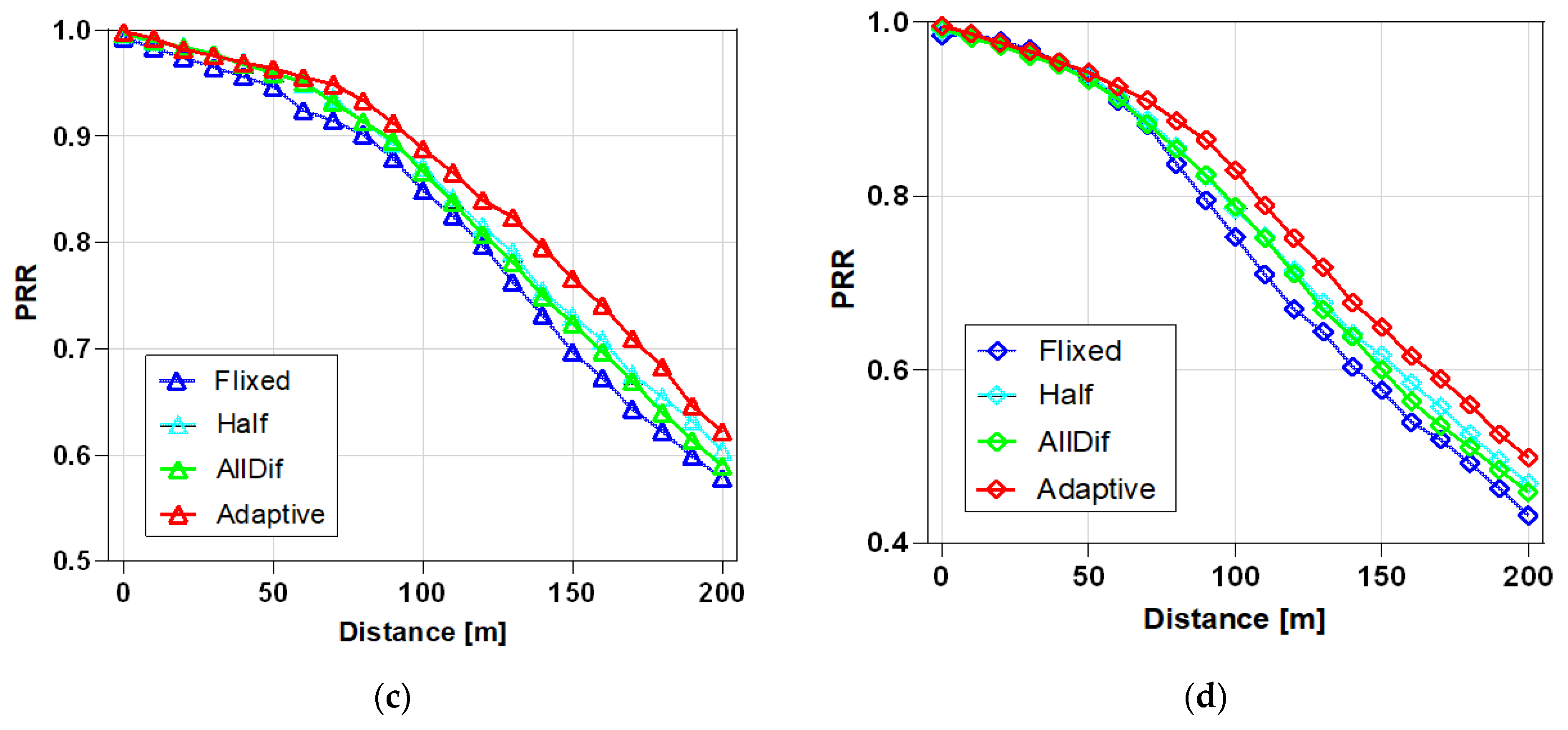
• The influence of vehicle speed on communication performance is analysed, considering the packet reception rate (PRR) and collision ratio (CR), especially in NR-V2X scenarios where vehicles and infrastructure coexist.
• An adaptive vehicle speed scheme based on the zone congestion level (CL) and inter-vehicle distance level (DL) is established to improve traffic efficiency and communication performance.
• The effectiveness of the adaptive vehicle speed in improving performance metrics is demonstrated.

The remaining paper is organised as follows. Section 2 describes the technologies relevant to this work. Section 3 outlines the proposed scheme. Section 4 presents the simulation settings and results. Section 5 presents the concluding remarks and highlights future research directions.

2. Related Work

Existing research on C-V2X has been focused on analysing and advancing the technological framework, the communication process and resource allocation mechanisms, data packet types, and the collaboration between various layers [14]. A comprehensive overview of the evolution of C-V2X technology based on 3GPP standards was provided in [15], highlighting the various technologies used for C-V2X communication, as well as the specific interfaces and communication methods. Another survey described the various data packet types and application scenarios in C-V2X [16]. The challenges associated with C-V2X and the issues that remain to be resolved for further development were discussed in [17]. In addition, the testing methods of V2X in the communication process were explored from an architectural perspective in [18]. The key performance indicators for four advanced use cases, including latency and reliability, were summarised in [19], and the authors compared vehicle stopping distances under different technical standards. The impact of autonomous vehicles (AVs) on traffic management was discussed in detail in [20], and the concept of saturation flow rate was proposed, which is defined as the maximum number of vehicles that can pass through a road per hour when the road is saturated. And the data shows that at the same speed, autonomous vehicles can significantly improve traffic capacity.

The safe distance between vehicles is one of the most important factors in ensuring road safety. A larger inter-distance allows drivers to have a longer reaction time, but it will reduce the road capacity. But a smaller ${Dis}_{inter}$ will increase the probability of collision. Some researchers [21] highlighted that the safety and performance stability of vehicle platoons depend on the gap (time or distance) maintained by vehicles in the same lane, which is defined by driver characteristics, highway geometric characteristics, and environmental factors. Considering these aspects, the authors discussed the application of cooperative adaptive cruise control (CACC) in future vehicle networks and analysed the challenges of combining vehicle network technology with CACC, considering three factors: information, driver characteristics, and control [22]. The driver’s braking reaction time (RT) and its influencing factors were studied in [23]. The reaction time is affected by many factors, including anticipation, urgency, age and gender, cognitive load, etc. Depending on the above factors, the RT ranges from 0.7 to 1.5 s. To test the vehicle communication performance in a vehicle platoon, an integrated simulator was developed [24] to assess the vehicle distance and speed. A method to modify the amplitudes and road design factors, in addition to the vehicle characteristics, in the conventional CAM algorithm was proposed [25], and the authors evaluated the effectiveness of speed recommendations based on the road environment in curve scenarios. Additionally, an innovative model that could capture the car-following behaviour of connected vehicles was developed, considering the communication probability [26]. The collaborative cooperation of vehicle lane changing and speed control in a designated area was analysed in [27]. Notably, in vehicle-following cases, communication and resource allocation between vehicles are crucial. Thus, a multi-hop communication mechanism, considering roadside users (RSUs) and the base station (BS) as relay nodes, was developed [28] to extend the data transmission range. A mechanism combining wireless resource allocation and transmission power configuration was established [29] to reduce power consumption, while increasing the number of vehicles in the formation. To satisfy latency and reliability requirements, some researchers analysed two dynamic resource allocation mechanisms [30]. Moreover, the performance of the sensing-based semi-persistent scheduling (SB-SPS) and random resource allocation algorithm in a platoon multicast scenario was evaluated [31], and the authors developed an algorithm based on the deep deterministic policy gradient to overcome the impact of local-based collaboration among vehicles, thereby reducing the conflict probability in resource selection. A scheme to improve resource allocation performance by configuring parameter values in SB-SPS was proposed in [32]. In addition, the mechanism of combining artificial intelligence algorithms was also studied in [33] to improve the communication performance of C-V2X.

3. Overview of Technologies

NR-V2X is a wireless communication technology introduced in Release 16. In addition to the traditional uplink (UL) and downlink (DL) communication links, NR sidelink (SL) links are defined in this framework [17]. The UL and DL support communication between the vehicle and BS through the Uu interface, while the SL allows direct communication through the PC5 interface. In addition to a broadcast mode, NR-V2X supports multicast and unicast modes to respond to advanced V2X use cases. The data packets transmitted in NR-V2X include both periodic and aperiodic types, with the SL data channels mainly including the physical sidelink control channel (PSCCH) and physical sidelink shared channel (PSSCH) [34]. The data packets, which contain basic information such as speed, position, and the surrounding environment, are carried by the PSSCH. Each data packet includes coordinated sidelink control information (SCI), with the two-stage SCI format used in NR-V2X. The first stage of SCI, containing general control information such as reserved resources and adopted modulation and coding schemes, is carried by the PSCCH. The second stage, carried by the PSSCH, contains private control information for the multicast and unicast modes.

NR-V2X supports two frequency ranges: frequency range 1 (FR1) and frequency range 2 (FR2) [35]. FR1, or sub-6 GHz, represents the range below 6 GHz, while FR2 refers to the range above 6 GHz, also known as the millimetre wave. The maximum bandwidths supported by FR1 and FR2 are 100 MHz and 400 MHz, respectively. The wireless frame structure is organised in both the time and frequency domains, with the minimum granularity being symbols and subcarriers, respectively [36]. Each frame contains 10 subframes, and the durations of the frame and subframe are 10 ms and 1 ms, respectively. To achieve lower latency, NR-V2X can support multiple numerologies, also known as subcarrier spacing (SCS). For SCS values of 15, 30, 60, and 120 kHz, the number of slots is 1, 2, 4, and 8, respectively. Each slot contains seven symbols with a normal cyclic prefix. The resource element is the smallest resource unit, consisting of one symbol in the time domain and one subcarrier in the frequency domain. Each resource block (RB) consists of 12 consecutive subcarriers with the same SCS. The number of resources required for packet transmission is determined by the physical layer parameter settings and packet size. The resource allocation mechanism in NR-V2X includes centralised and distributed modes [37]. In the centralised mode, the BS is responsible for resource management, requiring new resources for each transmission. In the distributed mode, users independently select resources using the SB-SPS, which allows users to reuse the same resources over several consecutive periods, thereby reducing the number of resource reselections [38]. First, users obtain the received signal strength indicator (RSSI) values of all resources in the sensing window with a duration of $T_{sensing}$ [39]. The resources that are occupied, with RSSI values exceeding the threshold, are excluded. Second, the best 20% of resources are identified to form the available resources list (${list}_a$), and one resource is randomly selected for data transmission. Next, a value between [5,15] is randomly generated as the reselection counter ($RC$), which indicates for how many periods the current resource can be continuously used. After each transmission, the $RC$ decreases by one. Finally, when the $RC$ reaches 0, the user needs to reselect resources. Specifically, users can either keep the current resource with probability $P_k$ or reselect new resources with probability (1−$P_k$). The value of $P_k$ ranges from 0 to 0.8.

A data packet is considered to be successfully received when the signal-to-interference-plus-noise ratio ($SINR$) at the receiver $K$, ${SINR}_K,$ exceeds the $SINR$ threshold ${SINR}_{TH}$. The ${SINR}_K$ at the receiver is calculated as follows:

$${SINR}_K=\frac{{RS}_K}{P_n+I_{M,K}}, [\mathrm{dB}]$$

(1)

$${RS}_K=\frac{P_{tx}\times G_r}{L\left({Dis}_{j,k}\right)}, [\mathrm{dB}]$$

(2)

where ${RS}_K$ is the received signal strength, calculated using Equation (2). $P_n$ is the noise power, and $I_{M,K}$ represents the cumulative interference from vehicles M using the same resources as transmitter $j$. $P_{tx}$ is the transmit power, $G_r$ denotes the antenna gain at the receiver, and $L$ is the path loss from transmitter to receiver [40]. ${Dis}_{j,k}$ is the distance between two vehicles. According to Equation (1), the success of data packet reception depends on the distance between the transmitter and receiver, as well as the number of vehicles using the same resource. Moreover, SB-SPS allows users to make independent resource selections, which increases the likelihood of users in similar environments selecting the same resources.

4. Adaptive Speed Scheme Based on Zone Congestion Level and Inter-Vehicle Distance Level

In this section, a detailed description of the proposed scheme is provided, including the scenario zoning, the calculation of $CL$ and $DL$, and the adaptive vehicle speed process.

4.1. Zone Division and Congestion Level in Each Zone

The simulation scenario in this article is a Manhattan or highway scenario, where vehicles and RSUs coexist. The RSU is located at the centre of the road and has a fixed position. Its main responsibility is to manage the number of vehicles in each zone and determine its $CL$. In this work, resource selection is performed in a distributed mode to allow vehicles to autonomously select resources. The entire scenario is evenly divided into several zones, as shown in Figure 1. The RSU calculates the number of vehicles in each zone based on the vehicle’s $X, Y$ coordinates. Vehicles in the same lane move in the same direction. The distance between two adjacent vehicles in the same lane is referred to as inter-vehicle distance, as shown by the pink arrow. Each black box represents a zone, with each zone’s range defined as the area between its left and right boundaries. Specifically, zone boundaries are determined according to the following equations.

$${left boundary}_{{zone}_i}=\left\{\begin{array}{c}\left(N_z-1\right)\ast {length}_{zone}, \\ \left(mod\left(i,N_z\right)-1\right)\ast {length}_{zone},\end{array}\begin{array}{c}mod\left(i,N_z\right)=0\\ else\end{array}\right.$$

(3)

$${right boundary}_{{zone}_i}=\left\{\begin{array}{c}{length}_{road}, \\ mod\left(i,N_z\right)\ast {length}_{zone},\end{array}\begin{array}{c}mod\left(i,N_z\right)=0\\ else\end{array}\right.$$

(4)

$${length}_{zone}={length}_{road} / N_z$$

(5)

where ${zone}_i$ represents the $i\mathrm{t}\mathrm{h}$ zone and $N_z$ is the number of zones in each direction, and the number is 4 for this work. ${length}_{road}$ is the road length, and ${length}_{zone}$ is the zone length, calculated using Equation (5). Assuming that the vehicle movement direction and located lane have been determined, the number of vehicles in each zone is based on the relationship between the vehicle’s X coordinate and zone boundary. The condition for vehicle $j$ to be in $i\mathrm{t}\mathrm{h}$ zone is

$$x_j\in \left[{left boundary}_{zon{e}_i},{right boundary}_{zon{e}_i}\right]$$

(6)

The threshold for the number of vehicles in zone ${TH}_v$ is determined using Equation (7), which indicates the maximum number of vehicles that can be accommodated in the zone while meeting the ${dis}_{safe}$ requirements. The safe distance ${dis}_{safe}$ is predefined, representing the minimum distance allowed between two vehicles. According to the driving rules, the safe distance is set based on the minimum allowable speed in the paper, converted to 3 s, with 25 m corresponding to 30 km/h.

$${TH}_v=⌈ {length}_{zone} / {dis}_{safe}⌉$$

(7)

The ratio between the actual number of vehicles $N_{v_{z_i}}$ in the $i\mathrm{t}\mathrm{h}$ zone and ${TH}_v$ is defined as ${Ratio}_{z_i}$. This value represents the relationship between the current number of vehicles and ${TH}_v$, and the ${CL}_i$ in the $i\mathrm{t}\mathrm{h}$ zone is determined by this value

$${Ratio}_{z_i}=(N_{v_{z_i}}-{TH}_v)/{TH}_v$$

(8)

$CL$ can be divided into three levels: congested, normal, and sparse. In addition, a tolerance rate ${CL}_{tolerate}$ is defined as 0.2 for a normal $CL$, indicating that ${Ratio}_{z_i}$ can be considered a normal $CL$ if this value is not exceeded.

$${CL}_i=\left\{\begin{array}{c}sparse,\\ normal,\\ congested,\end{array}\right. \begin{array}{c}{Ratio}_{z_i}\le 0\\ {Ratio}_{z_i}>0 \& {Ratio}_{z_i} \le {CL}_{tolerate} \\ else\end{array}$$

(9)

According to this discussion, a zone is considered sparse when there are fewer than ${TH}_v$ vehicles within it, normal when the number of vehicles exceeds ${TH}_v$ but not ${TH}_v$ * (1+${CL}_{tolerate}$), and congested otherwise.

4.2. Inter-Vehicle Distance Level

The position of a vehicle is represented by a set of X and Y coordinates, where X represents the horizontal position on the road, and Y represents the lane in which the vehicle is located. Because of the limitations of transmit power and road length, the maximum data packet transmission distance is specified as ${Dis}_t$, and only users within this range can receive the packet. As shown in Figure 2, x and y represent the vehicle location, and the circle denotes the ${Dis}_t$ of each vehicle. Users within the range ${Dis}_t$ are referred to as neighbours. For example, in Figure 2, the neighbours of V2 include V3, V4, and V5. The distance between any two vehicles j and k is calculated as follows:

$${dis}_{j,k}=\sqrt{{\left[\right(x_j-x_k)+(y_j-y_k\left)\right] }^2}$$

(10)

${Dis}_{inter}$ is related only to adjacent vehicles in the same lane. When all vehicles travel at the same speed, the distance between them is solely related to their initial positions, and the same ${Dis}_{inter}$ is maintained throughout the simulation. However, when different vehicle speeds are used, ${Dis}_{inter}$ varies, as shown in Figure 3. The Y coordinate of the vehicle is fixed, which means that vehicle lane changes are not considered in this work. The vehicle’s X coordinate is incremented by the product of the vehicle speed ${Speed}_j$ and time difference $T_{position}$ between the last position updates. The different speeds of all the vehicles result in different increments and thus, a varying ${Dis}_{inter}$.

$$X_j=X_j+{Speed}_j \ast T_{position}$$

(11)

${Dis}_{inter(j,k)}$ represents the distance between the front ($j$) and rear ($k$) vehicles. Because the Y coordinates of adjacent users in the same lane are the same, ${Dis}_{inter(j,k)}$ can be calculated using Equation (12):

$${Dis}_{inter(j,k)}=\sqrt{{(x_j-x_k)}^2}$$

(12)

The $DL$ of the $jth$ vehicle is determined according to the distance ${Dis}_{inter(j,k)}$ and ${dis}_{safe}$ calculated using Equation (13), and three levels of $DL$ are defined: large, normal, and small. In addition, a distance tolerance value ${DL}_{tolerate}$ is defined as 3 m. When the absolute difference between ${Dis}_{inter(j,k)}$ and ${dis}_{safe}$ is less than this value, the $DL$ is considered normal.

$${DL}_j=\left\{\begin{array}{c}large,\\ normal,\\ small,\end{array}\right. \begin{array}{c} ({Dis}_{inter(j,k)}-{dis}_{safe})>{DL}_{tolerate}\\ \left|{Dis}_{inter(j,k)}-{dis}_{safe}\right|\le {DL}_{tolerate} \\ ({Dis}_{inter(j,k)}-{dis}_{safe})<(-{DL}_{tolerate})\end{array}$$

(13)

Thus, when ${Dis}_{inter(j,k)}$ is smaller and larger than the distance within the tolerated safety range, the DL is considered small and large, respectively. ${Dis}_{inter(j,k)}$ within the tolerated safety range corresponds to the normal case. According to the state of ${DL}_j$, the distance between each vehicle and the vehicle in front can be obtained, providing a reference for the subsequent speed determination.

4.3. Adaptive Speed Based on Congestion Level and Inter-Vehicle Distance

The overall structure of the NR-V2X with the adaptive speed control scheme proposed in this study is shown in Figure 4. The entire simulation process consists of three parts: simulation initialisation, simulation loop, and adaptive speed.

The simulation initialisation process is shown in the left blue box of Figure 4. First is the parameter setting, including the physical layer, MAC layer, and resource allocation parameters. Next is initialisation of the vehicle position. The vehicle position follows a spatial Poisson distribution, and all vehicles have the initial speed. Finally, there is the zone division and congestion level of each zone.

The simulation loop, as shown in the yellow box in the middle of Figure 4, is the main module of the simulation, constrained by the simulation time $T_{sim}$. During each loop, the position of each vehicle must be updated periodically, and the neighbour update follows immediately. Then, the congestion level of each zone is updated and next entered into the proposed adaptive speed module to obtain the speed values. After that, the data transmission and resource selection are performed, and the key performance indicators, including PRR and CR, are updated. At the end of the simulation loop, the overall performance is output.

The adaptive speed control scheme, as shown in the green box on the right side of Figure 4, is implemented on a per-vehicle basis, and the speed of vehicle $j, { Speed}_j$, is provided based on ${CL}_i$ and ${DL}_j$. The speed is updated immediately after the vehicle position update, with a period $T_{speed}$. The allowed vehicle speeds in each zone include three settings: high speed $\left(Max\right)$, low speed $\left(Min\right)$, and maintaining the current speed $\left(maintain\right)$. When ${Dis}_{inter(j,k)}$ is large, $Max$ is used to reduce the distance as rapidly as possible, increasing the number of vehicles in the zone to improve transportation efficiency. When ${Dis}_{inter(j,k)}$ is excessively small, $Min$ is used to reduce the speed of the following vehicle to avoid collisions. When the distance between vehicles meets the ${dis}_{safe}$ requirements, the vehicle can maintain the current speed. The values of $Max$ and $Min$ differ depending on the zone $CL$, with less congested zones tolerating larger speed changes than zones with greater congestion. Overall, the $Max$ speed in sparse zones $\left({Max}_S\right)$ is the highest speed, while the $Min$ speed $\left({Min}_S\right)$ is the lowest speed. In normal zones, the $Max$ speed $\left({Max}_N\right)$ and $Min$ speed $\left({Min}_N\right)$ are intermediate speeds. In congested zones, the $Max$ speed $\left({Max}_C\right)$ and $Min$ speed $\left({Min}_C\right)$ are the lowest speeds. Hence, ${Max}_S$ > ${Max}_N$ > ${Max}_C$ and ${Min}_S$ > ${Min}_N$ > ${Min}_C$.

The adaptive speed control scheme for NR-V2X communication involves five steps:

Step 1: Scenario zones. According to Equations (3) and (4), the left and right boundaries of each zone are determined, and the road in each direction is divided into $N_z$ zones. The process of this step is outlined in the first part of Algorithm 1.

Step 2: Zone congestion level. Based on the vehicle’s X coordinate and zone boundary value, the number of vehicles in each zone is obtained using Equation (6). Then, ${Ratio}_{z_i}$ is obtained based on the number of vehicles and ${TH}_v$ in Equation (7). Finally, using Equation (9), the congestion level of each zone is determined based on the value of ${Ratio}_{z_i}$. This process is outlined in the second part of Algorithm 1.

Step 3: Vehicle zone. The zone in which the current vehicle is located is determined using Equation (6), and we obtain the congestion level of that zone, ${CL}_i$. This process is outlined in the first part of Algorithm 2.

Step 4: Inter-vehicle distance level. Using Equation (12), the ${Dis}_{inter(j,k)}$ between the current vehicle ($j$) and vehicle ($k$) in front is determined. Subsequently, ${DL}_j$ is obtained using Equation (13). This process is outlined in the second part of Algorithm 2.

Step 5: Vehicle speed. Based on ${CL}_i$, the speed equations, Equations (14)–(16), are selected for a sparse, normal, or congested ${CL}_i$, respectively. If ${DL}_j$ is too large, the speed should be $Max$; if it is normal, the speed should be $maintain$; and if ${DL}_j$ is too small, the speed should be $Min$. The details of this step are presented in Algorithm 3.

$${Speed}_j=\left\{\begin{array}{c}{Max}_S,\\ maintain,\\ {Min}_S,\end{array}\right. \begin{array}{c}{DL}_j is large ,\\ {DL}_j is normal,\\ {DL}_j is small ,\end{array}\mathit{if} {CL}_i \mathit{is} \mathit{sparse}$$

(14)

$${Speed}_j=\left\{\begin{array}{c}{Max}_N,\\ maintain,\\ {Min}_N,\end{array}\right. \begin{array}{c}{DL}_j is large ,\\ {DL}_j is normal,\\ {DL}_j is small ,\end{array}\mathit{if} {CL}_i \mathit{is} \mathit{normal}$$

(15)

$${Speed}_j=\left\{\begin{array}{c}{Max}_C,\\ maintain,\\ {Min}_C,\end{array}\right. \begin{array}{c}{DL}_j is large ,\\ {DL}_j is normal,\\ {DL}_j is small ,\end{array}\mathit{if} {CL}_i \mathit{is} \mathit{congested}$$

(16)

Considering these aspects, the range of speed values is first determined based on the congestion level of the zone in which the vehicle is currently located. The final specific speed is then determined based on the distance between each vehicle and the vehicle in front. Thus, both local and global information are used to determine the appropriate speed of each vehicle. The adaptive speed mechanism is based on the overall environment and individual vehicle state to set optimal speeds.

Algorithm 1: Scenario zone division and congestion level
1.	Scenario zones
2.	${length}_{road}$	🡠 Road length.
3.	$N_V$	🡠 Number of vehicles.
4.	$N_z$	🡠 Number of zones in each direction.
5.	for $i$ = $1:N$
6.	Follow Equations (4) and (5)
7.	${R\_b}_i$	🡠 Right boundary of the $i$th zone
8.	${L\_b}_i$	🡠 Left boundary of the $i$th zone.
9.	end
10.	Congestion level ($\mathit{C}\mathit{L}$)
11.	${Dis}_{safe}$	🡠 Safe distance.
12.	${TH}_V$ = $\frac{{length}_{road}}{N_z*{Dis}_{safe}}$	🡠 Threshold for the number of vehicles in zone.
13.	Follow Equation (6) to obtain $N_{v_{z_i}}$
14.	$N_{v_{z_i}}$	🡠 Number of vehicles in $i$th zone.
15.	${Ratio}_{z_i}$	🡠 Vehicle ratio for the $i$th zone.
16.	${Ratio}_{z_i}$ = $(N_{v_{z_i}}-{TH}_V)/{TH}_V$
17.	${CL}_i$	🡠 Congestion level of the $i$th zone.
18.	${CL}_{tolerate}$	🡠 Tolerance for zone congestion level.
19.	if ${Ratio}_{z_i}$ $\le$ 0
20.	${CL}_i$ is sparse
21.	elseif ${Ratio}_{z_i}$ $>$ 0 and ${Ratio}_{z_i}$ $\le$ ${CL}_{tolerate}$
22.	${CL}_i$ is normal
23.	else
24.	${CL}_i$ is congested
25.	end

Algorithm 2: Vehicle zone and inter-distance level
1.	Vehicle zone
2.	$V_{j_x}$, $V_{jy}$	🡠 X and Y coordinate of the $j\mathrm{t}\mathrm{h}$ vehicle.
3.	$z_{vj}$	🡠 Zone in which $j\mathrm{t}\mathrm{h}$ vehicle is located.
4.	if $V_{j\_x}$ $\in$ [${R\_b}_i$, ${L\_b}_i$]
5.	$z_{vj}$ = i;
6.	end
7.	Inter-vehicle distance level ($\mathit{D}\mathit{L}$)
8.	$V_j$, $V_k$	🡠 Current vehicle, vehicle ahead of $V_j$.
9.	${Dis}_{safe}$, ${DL}_{tolerate}$	🡠 Safe distance and tolerance for inter-distance level.
10.	${Dis}_{inter(j,k)}$	🡠 Inter-vehicle distance between $V_j$ and $V_k$ in the same lane.
11.	${Dis}_{inter(j,k)}$=$\sqrt{{\left(V_{j_x}-V_{k_x}\right)}^2}$
12.	${DL}_j$	🡠 Inter-distance level of $V_j$.
13.	if (${Dis}_{inter(j,k)}$ − ${Dis}_{safe}$) $>$ ${DL}_{tolerate}$
14.	${DL}_j$ is large
15.	elseif $\left|{Dis}_{inter(j,k)}-{Dis}_{safe}\right|$ $\le$ ${DL}_{tolerate}$
16.	${DL}_j$ is normal
17.	elseif (${Dis}_{inter(j,k)}$ − ${Dis}_{safe}$) $<$ (−${DL}_{tolerate}$)
18.	${DL}_j$ is small
19.	end

Algorithm 3: Adaptive speed based on $CL$ and $DL$
1.	Speed for  $V_j$
2.	${Max}_S$	🡠 High speed for the sparse zones.
3.	${Min}_S$	🡠 Low speed for the sparse zones.
4.	${Max}_N$	🡠 High speed for the normal zones.
5.	${Min}_N$	🡠 Low speed for the normal zones.
6.	${Max}_C$	🡠 High speed for the congested zones.
7.	${Min}_C$	🡠 Low speed for the congested zones.
8.	${CL}_i$	🡠 CL of the zone in which the $j\mathrm{t}\mathrm{h}$ vehicle is located.
9.	${DL}_j$	🡠 Inter-distance level of $V_j.$
10.	${Speed}_j$	🡠 Speed for $V_j$.
11.	if ${CL}_i$ is sparse or (normal) or [congested]
12.	if ${DL}_j$ is large
13.	${Speed}_j$ = ${Max}_S$ or (${Max}_N$) or [${Max}_C$];
14.	elseif ${DL}_j$ is normal
15.	${Speed}_j$ = maintain current speed;
16.	elseif ${DL}_j$ is small
17.	${Speed}_j$ = ${Min}_S$ or (${Min}_N$) or [${Min}_C$];
18.	end
19.	end

5. Simulation Setting and Results

Table 1. Parameter settings.

Parameter	Value
Scenario (Highway)
Lanes	One lane in each direction [42]
Length of road (${length}_{road}$)	2000 m [42]
Width (${width}_{road}$)	4 m [42]
Vehicle density ($\rho$)	50, 100, 150, and 200 vehicles/km [41]
Number of vehicles	$\rho$ * (${length}_{road}$) [41]
Vehicle initial speed	60 km/h [44,45]
Physical layer
Simulation time ($T_{Sim}$)	50 s [41]
Channels	ITS bands at 5.9 GHz [41]
Bandwidth	10 MHz [41]
Antenna gain ($G_r$)	3 dB [41]
Noise figure	9 dB [41]
Channel model	WINNER+, Scenario B1 [41]
Transmission power ($P_{tx}$)	23 dBm [43]
Modulation and coding scheme (MCS)	3 (QPSK, ${SINR}_{th}=1.0337 \mathrm{d}\mathrm{B}$) [34]
Subcarrier spacing (SCS)	15 kHz [36]
Subchannel size	10 RBs [41]
Resource allocation(SB-SPS)
Resource reservation interval (RRI)	100 ms [41]
Sensing duration ($T_{sensing}$)	1100 ms [41]
Resource sensing threshold ($P_{th}$)	−110 dBm [41]
Resource keeping probability ($P_k$)	0.4 [41]
Adaptive speed
Position and speed update interval ($T_{position}$, $T_{speed}$)	100 ms [41]
Safe distance (${dis}_{safe}$)	25 m [11]
High speed for sparse zones (${Max}_S$)	100 km/h [44,45]
Low speed for sparse zones (${Min}_S$)	50 km/h [44,45]
High speed for normal zones (${Max}_N$)	80 km/h [44,45]
Low speed for normal zones (${Min}_N$)	40 km/h [44,45]
High speed for congested zones (${Max}_C$)	70 km/h [44,45]
Low speed for congested zones (${Min}_C)$	30 km/h [44,45]

summarises the main parameter values used in the simulation. The simulations of this work were performed on the open-source system-level simulator WiLabV2Xsim [41]. The scenario is a highway setting, also known as a Manhattan scenario [42], where RSUs and vehicles coexist. Subsequently, the parameter values of the physical layer and resource selection algorithm are defined [41,43]. Finally, the setting of the proposed adaptive vehicle speed mechanism is provided. When different parameter values are used, the necessary explanation is provided. The performance evaluation metrics include the PRR and CR, defined as follows.

PRR: The ratio of the number of packets successfully received by the receiver to the total number of received packets.

CR: The ratio of the number of vehicle links where the inter-vehicle distance between the two vehicles is greater than the configured safety distance to the total number of vehicle links (i.e., links between two close vehicles in the same lane).

5.1. Impact of Vehicle Speed

This section first presents the performance under the conventional speed setting, where every vehicle moves at the same fixed speed. The PRR and CR values are shown in Figure 5a,b, respectively. The speed ranges from 20 to 120 in increments of 20 km/h (X-axis), and four densities are considered: 50, 100, 250, and 200 vehicles/km (presented in the legends). Furthermore, the setting of the safety distance is based on the requirement corresponding to the minimum speed allowed in the scenario. The lower the speed, the smaller the ${dis}_{safe}$, which can allow more vehicles to be accommodated in the zone and is more helpful for improving traffic efficiency.

Figure 5a shows that the total PRR decreases with increasing vehicle density, because higher vehicle densities lead to more conflicts over resource selection, resulting in more users selecting the same resources and increased interference. As described in Equation (1), the increase in $I_{M,K}$ results due to a larger $M$ reduces the probability of a data packet being successfully received. Furthermore, the PRR performance deteriorates as speed increases, particularly in higher densities. This is because the communication range (in which data can be received) includes neighbouring vehicles both in the same lane and parallel lanes, as shown in Figure 2. At high speeds, significant changes occur in vehicle positions and distances between parallel lanes. Consequently, the PRR performance degrades as the ${Dis}_{j,k}$ in Equation (2) increases with changes in the distance between vehicles in parallel lanes.

In contrast, at the same fixed speed, there is no significant variation in CR, as shown in Figure 5b. As the vehicles in the same lane maintain a constant ${Dis}_{inter(j,k)}$, as discussed previously, the CR is the same at all times. The CR in this case is extremely large, exceeding 50% in high-density scenarios. Thus, a fixed speed setting cannot reflect real mobility environments and does not enhance traffic efficiency.

5.2. Performance Comparison between Conventional and Adaptive Speed Schemes

This section presents a performance comparison of the conventional speed configuration and proposed adaptive speed scheme. Additionally, it presents comparative results for different vehicle speed configurations, to comprehensively analyse the performance changes caused by speed fluctuations under the $Half$ and $AllDif$ schemes. In the $Half$ scheme, half of the vehicles travel at ${Speed}_{Min}$ and the other half move at ${Speed}_{Max}$. In the $AllDif$ scheme, the speed of all vehicles is randomly generated within the speed range [${Speed}_{Min}$, ${Speed}_{Max}$]. The PRR and CR values are shown in Figure 6a,b, respectively, and the X-axis shows the four scenes with different vehicle densities. In the legend, $Fixed$ means that all vehicles use the same fixed speed; $Half$ refers to the use of two speed settings; $Alldif$ means that all vehicles have different speeds; and $Adaptive$ refers to the use of the proposed adaptive speed scheme. Speeds are defined as 60 km/h for $Fixed$, and ${Speed}_{Min}$ and ${Speed}_{Max}$ are 60 and 80 km/h for $Half$ and $AllDif$, respectively.

Overall, the performance deteriorates with increasing vehicle density. As discussed in the previous section, competition for resources intensifies, and the vehicles are more closely located as the number of users increases. Notably, different speeds indeed affect the performance. For example, the results of the $Half$ and $AllDif$ schemes are slightly improved compared with those for $Fixed$. This is because varying speeds allow the position increments to differ, which minimises the likelihood of position overlap and reduces resource selection conflicts in similar environments. However, the performance improvement is not significant, as both schemes exhibit comparable results. This is because, although $Half$ and $AllDif$ consider different vehicle speeds, the speeds are determined randomly and do not fully account for the vehicles’ current environment. Furthermore, the results indicate that the proposed adaptive speed mechanism provides the best performance in all scenarios. In particular, this mechanism effectively takes into account the zone congestion and ${Dis}_{inter}$ to provide reasonable speed recommendations. The most notable performance enhancement is observed at low vehicle densities, with the PRR approaching 1 and CR approaching 0. When the density is 50, 100, 150, and 200 vehicles/km, the number of vehicles in each direction is approximately 50, 100, 150, and 200, respectively. In each scenario, the average ${Dis}_{inter}$ that can support the even distribution of vehicles on a 2 km road is approximately 40, 20, 13, and 10 m, respectively. Low-density scenarios allow for a considerably higher ${Dis}_{inter}$ than ${dis}_{safe}$, resulting in fewer collisions. Additionally, resource competition is minimal when there are more resources than users. The application of an adaptive speed mechanism helps adjust ${Dis}_{inter}$, further reducing resource selection conflicts due to similar situations. In high-density scenarios, the possibility of resource reuse increases due to resource shortages. Second, the small ${Dis}_{inter}$ caused by vehicle oversaturation in the zone results in greater interference between users.

The detailed results of the four speed configurations will be elaborated to clarify the effectiveness of the proposed scheme. Figure 7 shows the change in CR with runtime. The four lines represent the four mechanisms, and (a)–(d) present the results obtained under the four vehicle densities.

Overall, a high density leads to a high CR. A fixed and identical speed setting does not cause the CR to fluctuate. As previously mentioned, a fixed-speed scenario maintains a fixed ${Dis}_{inter}$, and thus, the CR remains unchanged. The slight variations are attributable to the first vehicle on the road exiting and re-entering the scenario. Additionally, the CR performance varies slightly at different speed settings ($Half$ and $AllDif$). However, these schemes do not specifically consider the situation of each vehicle, leading to an unreasonable speed configuration in certain cases, resulting in a non-monotonically decreasing CR performance. In the case of the $Adaptive$ scheme, a higher CR is observed at the beginning, as ${Dis}_{inter}$ is identical and lower than ${dis}_{safe}$ due to the same initial positions. Over time, the CR decreases, because the $Adaptive$ method considers the $CL$ and $DL$ of each zone and vehicle to make corresponding speed adjustments. This demonstrates that the $Adaptive$ algorithm can assist vehicles in modifying their speed so that the inter-vehicle distances eventually conform to safety regulations. Moreover, in low-density scenarios, the traffic efficiency increases, and the CR can be maintained at 0 as time progresses. In addition, because the average safe distance permitted in the high-density scenarios is less than the necessary ${dis}_{safe}$ (for example, the average ${Dis}_{inter}$ is only 10 m in the case with 200 vehicles/km), the final CR of all schemes is constant. In other words, regardless of the scheme used, ${Dis}_{inter}$ is smaller than ${dis}_{safe}$ in some cases. One solution to address the problem is to reduce the number of users, and the alternative is to increase the road length. It is noteworthy that $Adaptive$ consistently maintains the highest performance.

Figure 8 shows the PRR performance as the distance between increases. As indicated in Equation (1), the $SINR$ decreases as the distance increases, leading to a higher probability of packets being incorrectly received. Consequently, the PRR decreases with increasing distance in all scenarios. However, $Adaptive$ can guarantee a higher PRR in each case, demonstrating that its objective is to obtain an appropriate safe ${Dis}_{inter}$ by adjusting speed rather than pursuing excessively large distances to reduce the collision rate. In addition, as indicated in Equation (1), the number of interfering vehicles that select the same resource as the transmitter, and their distance to the receiver, also influence the packet reception. More severe resource conflicts caused by a larger number of users increase the interference and reduce the PRR. Therefore, in the four density scenarios (Figure 8a–d), the PRR decreases as the density increases. As in the previous cases, $Adaptive$ outperforms the conventional schemes, even in high-density scenarios. This is because the proposed adaptive speed scheme reduces the probability of users overlapping at the same position (collision). Consequently, the RSSI values of the resources sensed by different users varies, and the overlap of ${list}_a$ is minimal when the vehicles use the SB-SPS algorithm for autonomous resource selection. The proposed scheme reduces the possibility of neighbours using the same resources and effectively avoids severe resource interference.

6. Conclusions

In this work, the impact of vehicle speed on communication performance and transportation efficiency in highway scenarios is studied. The content of this paper is similar to existing mechanisms that control the speed of vehicles in a platoon, like ACC and CACC. However, the main difference is that the proposed adaptive speed control scheme relies solely on NR-V2X communication and allows users to move at different speeds, which are adaptive based on inter-vehicle distance and congestion level. The analysis begins with the performance of data packet receipt and collision probability at the same or different vehicle speeds. Furthermore, an adaptive speed mechanism based on the $CL$ of zone and ${Dis}_{inter}$ is established. The proposed scheme makes suitable speed modifications that can effectively lessen collision probability, by considering the $CL$ in which the vehicle is currently located and distance between that vehicle and the front vehicle. Specifically, in low-density scenarios, the adaptive speed mechanism can provide a CR below 0.4, compared to 0.55 with conventional fixed-speed settings, representing a performance improvement of nearly 93%. Even in high-density scenarios, the proposed algorithm can offer a CR performance that is nearly 23% better than conventional settings. In addition, the proposed scheme can reduce resource selection conflicts between vehicles in similar environments, ensuring that data packets are received with a higher success rate. The adaptive speed scheme maintains a PRR above 0.9 in different density scenarios.

The objective of this work is to enhance communication performance between vehicles in the same lane and lower collisions. This paper only considers the speed variations of vehicles in the same lane in a highway scenario; therefore, future work will be aimed at analysing vehicle lane changes in multi-lane scenarios to improve traffic efficiency, and the application of the adaptive speed control scheme in urban scenarios will also be considered. Moreover, thanks to the efficiency and wide application of artificial intelligence algorithms, it is also a feasible direction to design more effective speed approaches utilizing reinforcement learning or optimisation algorithms.

References

1. 3rd Generation Partnership Project. Study on Evaluation Methodology of New Vehicle-to-Everything (V2X) Use Cases for LTE and NR; 3GPP TR 37.885 V15.3.0; 3GPP Support Office: Valbonne, France, 2019. [Google Scholar]
2. 3rd Generation Partnership Project. Technical Specification Group Radio Access Network; NR; NR and NG-RAN Overall Description; Stage 2; 3GPP TS 38.300 V 17.4.0; 3GPP Support Office: Valbonne, France, 2023. [Google Scholar]
3. ETSI Standard EN 302 637-2; Intelligent Transport Systems (ITS); Vehicular Communications; Basic Set of Applications; Part 2: Specification of Cooperative Awareness Basic Service. ETSI: Valbonne, France, 2014.
4. ETSI Standard EN 302 637-3; Intelligent Transport Systems (ITS); Vehicular Communications; Basic Set of Applications; Part 3: Specifications of Decentralized Environmental Notification Basic Service. ETSI: Valbonne, France, 2014.
5. 3rd Generation Partnership Project. Enhancement of 3GPP Support for V2X Scenarios; Stage 1; 3GPP TS 22.186 V17.0.0; 3GPP Support Office: Valbonne, France, 2022. [Google Scholar]
6. Brambilla, M.; Combi, L.; Matera, A.; Tagliaferri, D.; Nicoli, M.; Spagnolini, U. Sensor-Aided V2X Beam Tracking for Connected Automated Driving: Distributed Architecture and Processing Algorithms. Sensors 2020, 20, 3573. [Google Scholar] [CrossRef] [PubMed]
7. Bagheri, H.; Noor-A-Rahim, M.; Liu, Z.; Lee, H.; Pesch, D.; Moessner, K.; Xiao, P. 5G NR-V2X: Toward Connected and Cooperative Autonomous Driving. IEEE Commun. Stand. Mag. 2021, 5, 48–54. [Google Scholar] [CrossRef]
8. Cinque, E.; Valentini, F.; Persia, A.; Chiocchio, S.; Santucci, F.; Pratesi, M. V2X Communication Technologies and Service Requirements for Connected and Autonomous Driving. In Proceedings of the 2020 AEIT International Conference of Electrical and Electronic Technologies for Automotive (AEIT AUTOMOTIVE), Torino, Italy, 18–20 November 2020; pp. 1–6. [Google Scholar]
9. Kutila, M.; Pyykonen, P.; Huang, Q.; Deng, W.; Lei, W.; Pollakis, E. C-V2X Supported Automated Driving. In Proceedings of the 2019 IEEE International Conference on Communications Workshops (ICC Workshops), Shanghai, China, 20–24 May 2019; pp. 1–5. [Google Scholar]
10. Boubakri, A.; Gammar, S.M. Intra-platoon communication in autonomous vehicle: A survey. In Proceedings of the 2020 9th IFIP International Conference on Performance Evaluation and Modeling in Wireless Networks (PEMWN), Berlin, Germany, 1–3 December 2020; pp. 1–6. [Google Scholar]
11. Alalewi, A.; Dayoub, I.; Cherkaoui, S. On 5G-V2X Use Cases and Enabling Technologies: A Comprehensive Survey. IEEE Access 2021, 9, 107710–107737. [Google Scholar] [CrossRef]
12. Milanés, V.; Shladover, S.E.; Spring, J.; Nowakowski, C.; Kawazoe, H.; Nakamura, M. Cooperative Adaptive Cruise Control in Real Traffic Situations. IEEE Trans. Intell. Transp. Syst. 2014, 15, 296–305. [Google Scholar] [CrossRef]
13. Wang, Z.; Wu, G.; Barth, M.J. A Review on Cooperative Adaptive Cruise Control (CACC) Systems: Architectures, Controls, and Applications. In Proceedings of the 2018 21st International Conference on Intelligent Transportation Systems (ITSC), Maui, HI, USA, 4–7 November 2018; pp. 2884–2891. [Google Scholar]
14. Garcia, M.H.C.; Molina-Galan, A.; Boban, M.; Gozalvez, J.; Coll-Perales, B.; Şahin, T.; Kousaridas, A. A tutorial on 5G NR V2X communications. IEEE Commun. Surv. Tutor. 2021, 23, 1972–2026. [Google Scholar] [CrossRef]
15. Zhou, H.; Xu, W.; Chen, J.; Wang, W. Evolutionary V2X Technologies Toward the Internet of Vehicles: Challenges and Op-portunities. Proc. IEEE 2020, 108, 308–323. [Google Scholar] [CrossRef]
16. Soto, I.; Calderon, M.; Amador, O.; Urueña, M. A Survey on Road Safety and Traffic Efficiency Vehicular Applications Based on C-V2X Technologies. Veh. Commun. 2022, 33, 100428. [Google Scholar] [CrossRef]
17. MacHardy, Z.; Khan, A.; Obana, K.; Iwashina, S. V2X Access Technologies: Regulation, Research, and Remaining Challenges. IEEE Commun. Surv. Tutor. 2018, 20, 1858–1877. [Google Scholar] [CrossRef]
18. Wang, J.; Shao, Y.; Ge, Y.; Yu, R. A Survey of Vehicle to Everything (V2X) Testing. Sensors 2019, 19, 334. [Google Scholar] [CrossRef]
19. Ganesan, K.; Lohr, J.; Mallick, P.B.; Kunz, A.; Kuchibhotla, R. NR Sidelink Design Overview for Advanced V2X Service. IEEE Internet Things Mag. 2020, 3, 26–30. [Google Scholar] [CrossRef]
20. Wiseman, Y. Autonomous vehicles will spur moving budget from railroads to roads. Int. J. Intell. Unmanned Syst. 2024, 12, 19–31. [Google Scholar] [CrossRef]
21. Dey, K.C.; Yan, L.; Wang, X.; Wang, Y.; Shen, H.; Chowdhury, M.; Yu, L.; Qiu, C.; Soundararaj, V. A Review of Communi-cation, Driver Characteristics, and Controls Aspects of Cooperative Adaptive Cruise Control (CACC). IEEE Trans. Intell. Transp. Syst. 2016, 17, 491–509. [Google Scholar] [CrossRef]
22. Li, Y.; Wang, H.; Wang, W.; Xing, L.; Liu, S.; Wei, X. Evaluation of the Impacts of Cooperative Adaptive Cruise Control on Reducing Rear-End Collision Risks on Freeways. Accid. Anal. Prev. 2017, 98, 87–95. [Google Scholar] [CrossRef] [PubMed]
23. Summala, H. Brake reaction times and driver behavior analysis. Transp. Hum. Factors 2000, 2, 217–226. [Google Scholar] [CrossRef]
24. Choudhury, A.; Maszczyk, T.; Asif, M.T.; Mitrovic, N.; Math, C.B.; Li, H.; Dauwels, J. An Integrated V2X Simulator with Applications in Vehicle Platooning. In Proceedings of the 2016 IEEE 19th International Conference on Intelligent Transportation Systems (ITSC), Rio de Janeiro, Brazil, 1–4 November 2016; pp. 1017–1022. [Google Scholar]
25. Aznar-Poveda, J.; Egea-Lopez, E.; Garcia-Sanchez, A.-J.; Garcia-Haro, J. Advisory Speed Estimation for an Improved V2X Communications Awareness in Winding Roads. In Proceedings of the 2020 22nd International Conference on Transparent Optical Networks (ICTON), Bari, Italy, 19–23 July 2020; pp. 1–4. [Google Scholar]
26. Li, Y.; Chen, W.; Peeta, S.; Wang, Y. Platoon Control of Connected Multi-Vehicle Systems Under V2X Communications: De-sign and Experiments. IEEE Trans. Intell. Transp. Syst. 2020, 21, 1891–1902. [Google Scholar] [CrossRef]
27. Yan, S.; Wang, J.; Wang, J. Coordinated Control of Vehicle Lane Change and Speed at Intersection under V2X. In Proceedings of the 2018 3rd International Conference on Mechanical, Control and Computer Engineering (ICMCCE), Huhhot, China, 14–16 September 2018; pp. 69–73. [Google Scholar]
28. Zhou, S.; Wu, Q.; Tan, G.; Yang, D.; Ni, B. On Performance of Cooperative V2X Communication with Vehicular Platoon Systems. In Proceedings of the 2021 IEEE 23rd Int Conf on High Performance Computing & Communications; 7th Int Conf on Data Science & Systems; 19th Int Conf on Smart City; 7th Int Conf on Dependability in Sensor, Cloud & Big Data Systems & Application (HPCC/DSS/SmartCity/DependSys), Haikou, China, 20–22 December 2021; pp. 955–960. [Google Scholar]
29. Wang, P.; Di, B.; Zhang, H.; Bian, K.; Song, L. Platoon cooperation in cellular V2X networks for 5G and beyond. IEEE Trans. Wirel. Commun. 2019, 18, 3919–3932. [Google Scholar] [CrossRef]
30. Nardini, G.; Virdis, A.; Campolo, C.; Molinaro, A.; Stea, G. Cellular-V2X Communications for Platooning: Design and Evalu-ation. Sensors 2018, 18, 1527. [Google Scholar] [CrossRef]
31. Cao, L.; Roy, S.; Yin, H. Resource Allocation in 5G Platoon Communication: Modeling, Analysis and Optimization. IEEE Trans. Veh. Technol. 2023, 72, 5035–5048. [Google Scholar] [CrossRef]
32. Yin, J.; Hwang, S.-H. Adaptive Sensing-Based Semipersistent Scheduling with Channel-State-Information-Aided Reselection Probability for LTE-V2V. ICT Express 2022, 8, 296–301. [Google Scholar] [CrossRef]
33. Lei, L.; Liu, T.; Zheng, K.; Hanzo, L. Deep reinforcement learning aided platoon control relying on V2X information. IEEE Trans. Veh. Technol. 2022, 71, 5811–5826. [Google Scholar] [CrossRef]
34. 3rd Generation Partnership Project. NR; Physical Channels and Modulation; 3GPP TS 38.211 V18.2.0; 3GPP Support Office: Valbonne, France, 2024. [Google Scholar]
35. 3rd Generation Partnership Project. NR; Requirements for Support of Radio Resource Management; 3GPP TS 38.133 V18.3.0; 3GPP Support Office: Valbonne, France, 2023. [Google Scholar]
36. 3rd Generation Partnership Project. NR; Physical Layer Procedures for Data; 3GPP TS 38.214 V16.7.0; 3GPP Support Office: Valbonne, France, 2021. [Google Scholar]
37. 3rd Generation Partnership Project. 2X Services Based on NR; User Equipment (UE) Radio Transmission and Reception; 3GPP TR 38.886 V16.3.0; 3GPP Support Office: Valbonne, France, 2023. [Google Scholar]
38. 3rd Generation Partnership Project. Overall Description of Radio Access Network (RAN) Aspects for Vehicle-to-Everything (V2X) Based on LTE and NR; 3GPP TR 37.985 V17.1.1; 3GPP Support Office: Valbonne, France, 2022. [Google Scholar]
39. 3rd Generation Partnership Project. NR; Physical Layer Measurements; 3GPP TS 38.215 V17.3.0; 3GPP Support Office: Valbonne, France, 2023. [Google Scholar]
40. 3rd Generation Partnership Project. Study on Channel Model for Frequencies from 0.5 to 100 GHz; 3GPP TR 38.901 V18.0.0; 3GPP Support Office: Valbonne, France, 2024. [Google Scholar]
41. Todisco, V.; Bartoletti, S.; Campolo, C.; Molinaro, A.; Berthet, A.O.; Bazzi, A. Performance analysis of sidelink 5G-V2X mode 2 through an open-source simulator. IEEE Access 2021, 9, 145648–145661. [Google Scholar] [CrossRef]
42. 3rd Generation Partnership Project. Study on Scenarios and Requirements for Next Generation Access Technologies; 3GPP TR 38.913 V16.0.0; 3GPP Support Office: Valbonne, France, 2020. [Google Scholar]
43. 3rd Generation Partnership Project. User Equipment (UE) Radio Transmission and Reception; Part 1: Range 1 Standalone; 3GPP TS 38.101 V17.3.0; 3GPP Support Office: Valbonne, France, 2021. [Google Scholar]
44. 3rd Generation Partnership Project. NR; Study on NR Vehicle-to-Everything (V2X); 3GPP TS 38.885 V16.0.0; 3GPP Support Office: Valbonne, France, 2019. [Google Scholar]
45. 3rd Generation Partnership Project. Service Requirements for V2X Services; Stage 1; 3GPP TS 38.101 V17.3.0; 3GPP Support Office: Valbonne, France, 2022. [Google Scholar]
Figure 1. Scenario zone division.
Electronics 13 02678 g001
Figure 2. Vehicle position and transmission distance.
Electronics 13 02678 g002
Figure 3. Varying inter-vehicle distances with different speeds (a) at time t i and (b) at time t j .
Electronics 13 02678 g003
Figure 4. Simulation structure of adaptive speed scheme based on zone congestion and inter-vehicle distance level.
Electronics 13 02678 g004
Figure 5. PRR and CR performance with fixed vehicle speed. (a) PRR vs. density and (b) CR vs. density.
Electronics 13 02678 g005
Figure 6. PRR and CR performance with fixed, H a l f , A l l D i f , and adaptive vehicle speed schemes. (a) PRR vs. vehicle density and (b) CR vs. vehicle density.
Electronics 13 02678 g006
Figure 7. CR performance vs. time when vehicle density is (a) 50 vehicles/km, (b) 100 vehicles/km, (c) 150 vehicles/km, and (d) 200 vehicles/km.
Electronics 13 02678 g007
Figure 8. PRR performance vs. distance. (a) 50 vehicles/km, (b) 100 vehicles/km, (c) 150 vehicles/km, and (d) 200 vehicles/km.
Electronics 13 02678 g008aElectronics 13 02678 g008b