A Multivariate Time Series Prediction Method for Automotive Controller Area Network Bus Data

Abstract

This study addresses the prediction of CAN bus data, a lesser-explored aspect within unsupervised anomaly detection research. We propose the Fast-Gated Attention (FGA) Transformer, a novel approach designed for accurate and efficient prediction of CAN bus data. This model utilizes a cross-attention window to optimize computational scale and feature extraction, a gated single-head attention mechanism in place of multi-head attention, and shared parameters to minimize model size. Additionally, a generalized unbiased linear attention approximation technique speeds up attention block computation. On three datasets—Car-Hacking, SynCAN, and Automotive Sensors—the FGA Transformer achieves predicted root mean square errors of 1.86 × 10⁻³, 3.03 × 10⁻³, and 30.66 × 10⁻³, with processing speeds of 2178, 2768, and 3062 frames per second, respectively. The FGA Transformer provides the best or comparable accuracy with a speed improvement ranging from 6 to 170 times over existing methods, underscoring its potential for CAN bus data prediction.

1. Introduction

Modern automobiles are increasingly perceived as sophisticated computing systems rather than mere mechanical entities, especially in the context of smart vehicles. These vehicles are equipped with a multitude of sensors and Electronic Control Units (ECUs) that are interconnected through the Controller Area Network (CAN) bus. As intelligent automotive systems continue to advance, the trend toward Vehicle-to-Everything (V2X) communications is escalating the complexity of CAN bus data. As a broadcasting-based bus network without authentication, CAN technology provides access to thousands of sensors and signals, with a data volume reaching several gigabytes per hour. Consequently, the study of CAN bus data has emerged as a focal point for academic research. These data can be used to investigate and understand various issues, including traffic congestion, vehicle energy consumption and emissions, vehicle anomaly detection [1], and driver behavior [2].

The practical applications of CAN bus data analysis are vast and impactful. For instance, predictive maintenance strategies leveraging CAN bus data can anticipate component failures before they lead to breakdowns, enhancing vehicle reliability and safety. Fuel efficiency optimization, achieved through real-time analysis of driving habits and engine performance, not only reduces environmental impact but also saves on operational costs. Advanced driver-assistance systems (ADASs) rely on accurate CAN bus data prediction to improve their effectiveness, potentially preventing accidents on the road. Additionally, traffic management systems can utilize CAN bus data to alleviate congestion and improve overall traffic flow, while vehicle diagnostics can be swiftly and accurately performed, leading to more efficient repairs and maintenance. Insurance companies can also benefit by offering customized policies based on driver behavior and vehicle condition. Furthermore, the rapid development of autonomous vehicles hinges on the precise prediction of CAN bus data for reliable operation. Lastly, cybersecurity measures can be strengthened by monitoring CAN bus data for any signs of unauthorized access or manipulation, protecting vehicles from cyber threats.

In recent years, there has been a surge of research dedicated to the prediction of CAN bus data. Numerous studies have endeavored to perform unsupervised anomaly detection through predictive or reconstructive methods [3,4,5,6,7,8,9,10,11,12,13]. Unlike supervised anomaly detection techniques [14,15,16], these approaches do not necessitate the collection of costly anomaly data. However, these methods often place a greater emphasis on anomaly detection capabilities than on the accuracy of data predictions. We think it is necessary to study a real-time prediction method, as it is instrumental in recovering data from anomalies to ensure the vehicle’s normal operation.

Although there are relatively few direct studies on CAN bus data prediction, the fundamental principles underlying these methods are consistent with those employed in unsupervised anomaly detection. This consistency is primarily manifested in the thorough understanding and learning of the unique features inherent in CAN bus data. For instance, ref. [3] introduces an anomaly detection technique for CAN bus traffic using the bzip2 compression algorithm, extracting crucial information via bzip2 and identifying anomalies through similarity assessments. A deep auto-encoder neural network [4] is used to reconstruct the 20 Hz sampled CAN bus data. The CANet [5] model introduces an independent Long Short-Term Memory (LSTM) input model for each identifier (ID), employing an auto-encoder to facilitate interaction and reconstruction of CAN bus data. However, as the number of CAN devices grows, the model complexity of the CANet grows rapidly. LSTM [6] is used to study CAN bus data represented as 64 bits. The CLAM model [7] uses convolution to extract the features of the CAN signal, and the Bi-directional Long Short-Term Memory (Bi-LSTM) is used to extract time features. These time attention mechanisms aim to focus on important time steps. The CLAM model demonstrates better convergence speed and prediction accuracy than the original LSTM. Another Bi-LSTM model [8] has been presented for vehicle intrusion detection systems with a Synthetic Minority Over-sampling Technique (SMOTE) under-sampling strategy for handling imbalanced data. A Generative Adversarial Network (GAN) [9] is proposed for the self-supervised classification of anomalous CAN bus data. However, the generator of the GAN is used to generate abnormal data, not to extract features of normal data. Therefore, this network cannot be used to predict normal CAN bus data. In [10], an auto-encoder is used to learn the optimal features from CAN packets, and a Gaussian mixture model is used to cluster the CAN bus data into normal and anomalous categories. Four different network structures, each stacking a Convolutional Neural Network (CNN) followed by single-layer LSTM [11], are designed to learn the features of CAN bus data. Ref. [12] proposes a method that clusters CAN IDs based on signal correlation and utilizes the multiple Temporal Convolutional Network (TCN) to predict CAN bus data in different groups, which can also classify anomalies through thresholding. The AMAEID model [13] employs a multi-layer denoising auto-encoder to extract features from binary CAN data. The above methods utilize different CAN bus data preprocessing methods and different datasets. Additionally, some methods are more focused on reconstructing the data rather than prediction. Although these methods can learn the characteristics of CAN bus data, the prediction accuracy is challenging to compare and evaluate.

Table 1. Existing methods for CAN bus data analysis.

Methods	Datasets	Key Findings	Limitations
Anomaly detection using bzip2 compression [3]	Car-Hacking dataset	Extracts crucial info via bzip2; identifies anomalies through similarity assessments	Unable to detect replay attacks
Deep auto-encoder neural network [4]	20 Hz sampled CAN bus data	Reconstructs CAN bus data for anomaly detection	Can only process sampled data
CANet with LSTM and auto-encoder [5]	SynCAN	Facilitates interaction and reconstruction of CAN bus data	Model complexity grows with number of CAN devices
LSTM [6]	Binary and Hexadecimal CAN Bus Data	Studies CAN bus data with LSTM	Limited by the sequential nature of LSTM
CLAM model with convolution and Bi-LSTM [7]	Physical CAN signals	Conv1D to extract the abstract features of the signal values at each time step and Bi-LSTM to extract the time dependence	Processes each ID separately without correlation
Bi-LSTM with SMOTE under-sampling [8]	Attack and Defense Challenge-2020	The SMOTE under-sampling strategy is used to address the issue of imbalanced data	Unable to recover from error
Generative Adversarial Network (GAN) [9]	Car-Hacking dataset	Utilizes pseudo data to assist the network in learning normal data features	Cannot detect system errors
Auto-encoder with Gaussian mixture model [10]	CAN IDs; KDDCup-99; WSN-DS; ISCX	GMM is employed to cluster the CAN packet data into normal and attacks	Clustering may lead to misclassifications
CNN-LSTM stacked networks [11]	Car-Hacking dataset	End-to-end approach with no need to extract manual features	Processes each ID separately without correlation
Clustering and TCN for prediction [12]	SynCAN; Crysys dataset of can traffic logs	Combines correlation analysis with time series forecasting	Misgrouping of IDs may lead to severe misinterpretation
AMAEID with multi-layer denoising auto-encoder [13]	Binary CAN data	A multi-layer denoising auto-encoder model and the attention mechanism are used	The massive attacks may make the AMAEID model fail

summarizes the methods, datasets, key findings, and limitations of these methods.

CAN bus data can be viewed as multi-dimensional time series data, with each signal occupying a different dimension. Therefore, methods developed for time series data can be applied to solve the CAN bus data problem. A Convolutional Autoencoder (CAE) for feature extraction combined with LSTM for time series prediction is proposed in [17], demonstrating significantly lower prediction error compared to other models when applied to noisy time series data. A dual-head attention model with a bidirectional Gated Recurrent Unit (GRU) [18] has been used for water quality data imputation. MDST-GNN [19] is a multivariate time series deep spatiotemporal forecasting model that incorporates a Graph Neural Network (GNN) to enhance the accuracy of periodic data prediction. PSTA-TCN [20] combines a parallel spatiotemporal attention mechanism with stacked temporal convolutional networks to extract features from multivariate time series with varying window sizes. DAFA-BiLSTM [21] combines the benefits of a pretraining vector autoregression mechanism with an efficient representation of both linear and nonlinear features. It learns nonlinear feature information from multiple perspectives while generating a hierarchical feature representation. A hybrid GARCH-ATT-LSTM model [22] is proposed for non-stationary time series analysis and forecasting in financial datasets, leveraging Generalized Auto-Regressive Conditional Heteroskedasticity (GARCH) for volatility, attention for data prioritization, and LSTM for price predictions, outperforming baseline models in accuracy and interpretability. Ref. [23] presents a network architecture integrating a RNN and CNN to process and analyze multimodal data for quality control purposes in industrial production processes. A GNN based on multi-scale temporal feature extraction and attention mechanisms [24] has been proposed for multivariate time series prediction.

In the context of understanding CAN bus data, the auto-encoder structure has demonstrated significant advantages. The attention mechanism has become one of the most crucial methods in time series data research, offering valuable insights for the study of CAN bus data. However, the application of CAN bus data is constrained by privacy protection measures, preventing it from being uploaded to the cloud. Moreover, the limited computational resources at the vehicle’s end and the need for real-time performance impose high demands on the methodologies employed, which in turn limit the use of attention mechanisms in understanding CAN bus data. Therefore, when considering prediction accuracy, it is also necessary to consider the complexity of the algorithm to meet the real-time computing needs at the vehicle end.

This paper proposes the fast-gated attention mechanism (FGA Transformer), an innovative Transformer network designed for rapid and precise feature extraction in the prediction of CAN bus data. The key novel aspects of the FGA Transformer are as follows:

First, we introduce a unique cross-attention window for multi-dimensional time series data, which captures the intricate correlations and historical information within CAN bus data. Using a 1D pooling layer, this window effectively increases the temporal receptive field, enhancing feature extraction across multiple attention modules.

Second, the FGA mechanism, a core component of our network, comprises a gated self-attention mechanism and a generalized unbiased linear attention approximation. This gated single-head attention design not only shares weights between self-attention and global attention but also takes advantage of a generalized linear approximation to significantly accelerate inference.

Third, extensive experimental validation confirms the FGA Transformer’s outstanding prediction accuracy and speed, particularly when processing complex CAN bus data.

These enhancements make the FGA Transformer a good solution for the timely and accurate analysis of CAN bus data, contributing valuable insights to the field of unsupervised anomaly detection.

The remainder of this paper is structured as follows. In Section 2, we describe the CAN bus data and the Transformer method. In Section 3, we explain the FGA Transformer in more detail. In Section 4, we describe the experimental evaluation and results. In Section 5, we briefly discuss two practical implementation approaches for real-world scenarios. In Section 6, we present our conclusions and suggestions for future work.

2. Backgrounds

In this section, we offer brief overviews of CAN bus data and the multi-head attention mechanism in the Transformer method for analyzing high-dimensional time series data.

2.1. CAN Bus Data

The CAN bus network is a message-based broadcast protocol and is designed to allow ECUs to communicate with each other. A standard CAN message format is shown in Figure 1, which is composed of the following fields: Start of Frame (SOF), identifier (CAN ID), Remote Transmission Request (RTR), reserved, Data Length Code (DLC), Data Field, Cyclic Redundancy Check (CRC), Acknowledge (ACK) and End of Frame (EOF).

The two most relevant fields for this work are the identifier and the data payload. These data are not independent but collectively describe the vehicle states and driving behaviors in the same scene. However, the data are encoded according to different formats, which depend on the specific design choices operated by the original equipment manufacturer, and the encoding method is nonpublic information [25,26]. Without the manufacturer’s help, it is troublesome to find the corresponding relationship between real ECUs and IDs. Understanding the meaning of data payload is also a difficult task. This lack of prior knowledge has significant disadvantages in understanding CAN bus data by manual rules.

Although many devices send data to the CAN bus at uniform intervals, the intervals between signals from different devices are not uniform. Furthermore, the occurrence of control signals does not have a fixed time interval. Therefore, the overall CAN bus data are non-uniformly spaced, which also limits the application of many time series data processing methods.

2.2. Transformer for Multi-Dimensional Time Series Data

The Transformer [27] is an encoder and decoder network based on multi-headed attention mechanisms, without recurrence and convolutions. It is first applied to natural language processing problems and soon expands its application field to images, point clouds, multi-dimensional time series data, etc.

The training sample $X_t=\left\{x_{t,1},\dots ,x_{t,L_x}|x_{t,i}\in {ℝ}^{d_x}\right\}$ is defined as multi-dimensional time series data at the time $t$, input length $L_x$, and dimension $d_x$, and the output is $Y_t=\left\{y_{t,1},\dots ,y_{t,L_y}|y_{t,i}\in {ℝ}^{d_y}\right\}$ with a forecasting horizon $L_y$ and output dimension $d_x$.

Multi-headed attention is calculated as follows:

$$output=relu\left(MultiHead\times W^{O_1}\right)W^{O_2}$$

(1)

$$MultiHead=concat\left(hea{d}_1,\dots ,hea{d}_H\right)W^M$$

(2)

$$hea{d}_h=softmax\left(\frac{Q_h{K}_h^T}{\sqrt{d_k}}\cdot M\right)V_h,h=1,\dots ,H$$

(3)

$$Q_h=X{W}_h^Q$$

(4)

$$K_h=X{W}_h^K$$

(5)

$$V_h=XW$$

(6)

$$d_k=d/H$$

(7)

where $Q_h,K_k,V_h$ are the learnable query matrices, key matrices, and value matrices of the $h$ head, $M$ is the mask matrix, and $W^{*}$ are weights of a linear layer.

3. FGA Transformer

In this section, the network structure and implementation method of the proposed method, FGA Transformer, are introduced.

Table 2. Details of FGA Transformer prediction process.

Pre-Processing: Extract the CAN IDs and mapping them to the range [0, num(id)] Normalize the timestamps

Spatiotemporal Encoding: Convert the CAN data into a sparse matrix according to ID (Equations (8) and (9)) Calculate the encoding offsets $p_{t,i}$ based on timestamp and ID (Equations (12) and (13)) The CAN data are added to $p_{t,i}$ through a linear layer (Equation (11))

Local Attention and Global Attention Stack × N: Extract data based on a cross-window after one-dimensional max pooling (Equation (14)) Accumulate data from multiple timestamps as global data based on the group size Calculate global Q, K and local Q, K separately (Equations (19) and (20)) Calculate shared weights V and Gate (Equations (21) and (25)) Calculate global attention and local attention separately (Equation (17)) Calculate the total attention (Equations (28) or (29)) Restore cross-window data to normal data

Output: Output prediction results after passing through a linear layer

shows the prediction pipeline for the CAN data, detailing the sequence of operations from data input to prediction output.

3.1. Overall Architecture

The overall architecture of our proposed FGA Transformer is illustrated in Figure 2. The FGA Transformer shares a similar topology to the original Transformer encoder, differing in three key aspects:

• We employ a novel encoding method by calculating absolute ID information and relative timestamps;
• A cross-window block is proposed to process multi-dimensional time series data, characterizing both the spatial and long-term temporal dimensions;
• It replaces the multi-head self-attention mechanism with our proposed single-head FGA mechanism.

3.2. Pre-Processing and Spatiotemporal Encoding

We have conducted a thorough pre-processing of the CAN bus data to ensure the quality and relevance of the training dataset. This pre-processing for the dataset preparation phase involved several key steps:

Data Acquisition: the CAN bus data were collected using a bus logger that was connected to the vehicle’s On-Board Diagnostics (OBD) interface.

Data Cleaning: To ensure the integrity of the data, we conducted a thorough cleaning process. This involved the removal of any data that did not conform to the CAN bus protocol, such as incorrectly formatted messages or messages with missing or invalid fields. These anomalies in the data could be easily detected through format validation, which suggests that there is no need to burden the neural network with the task of identifying and correcting these anomalies in the incorrectly formatted data.

CAN ID Filtering: We identified and removed CAN IDs that appeared infrequently in the dataset. Specifically, we excluded CAN IDs that were present in only a single digit across tens of thousands of frames, aiming to minimize the influence of rare data on the network’s learning process. Rare CAN IDs may introduce noise and hinder the model’s ability to generalize to real-world scenarios. By filtering out these IDs, we focused our analysis on the most commonly occurring and relevant data, thereby enhancing the model’s predictive power. In fact, the filtering of infrequent CAN IDs is a standard step in the creation of CAN bus datasets.

After the above steps, the core content of standard CAN bus data is represented in

Table 3. CAN bus data examples.

ID	Timestamp	Data
0350	1479121434.850202	05 28 84 66 6d 00 00 a2
02c0	1479121434.850423	14 00 00
0430	1479121434.850977	03 80 00 ff 21 80 00 9d
…	…	…

, including the CAN ID, timestamp, and data load, where the CAN ID and data load are hexadecimal. The meaning of data load and the correspondence between the ID and device are unknown.

It is crucial to clarify that the above steps should be conducted during the dataset preparation phase. Conversely, the following four steps should be carried out during each training and inference session.

CAN ID Mapping: To make the calculation easier, we converted the hexadecimal data into decimal data. The decimal IDs are sparsely distributed between 0 and 65535, which means that only dozens of IDs are used in 0–65535. To ensure the validity of the spatial encoding, it is necessary to map the IDs to $\left[0,num\left(id\right)\right]$.

Segmentation: We segmented the normalized CAN bus data into smaller sequences, each of which is of a fixed length. These sequences were then used to train and validate the neural network models. Shorter slices are faster but may miss key temporal patterns, while longer slices capture more detail but require more processing power. The optimal slice length is determined by the available computational resources and the desired accuracy of the neural network models.

Sparsification: For CAN bus data $dat{a}_t=\left[id,timestamp,data\right]$, the constructed multi-dimensional time series data $X_t$ are

$$X_t=\left\{x_{t,1},\dots ,x_{t,L_x}|x_{t,i}\in {ℝ}^{d_x}\right\}$$

(8)

$$x_{t,i}=\left\{\begin{array}{l}data, \mathrm{if} {\mathit{id}}_{t,i} \mathrm{exists} \mathrm{at} {\mathit{timestamp}}_t\hfill \\ 0, \mathrm{else}\hfill \end{array}\right.$$

(9)

where $X_t$ is a sparse matrix. We tried to learn the CAN bus data directly, similar to natural language processing, rather than converting them into a sparse matrix. However, the results are poor. We suspect this is because the similarity within CAN bus data is much higher than that within natural language, and thus the requirement for prediction accuracy is higher. In Section 4.4, we present the results of the pre-processing methods, which further demonstrate these challenges.

Encoding: When extracting features, the Transformer considers the order of the features by positional encodings. Therefore, we used timestamp and ID information to encode the features, which can maximize the network’s sensitivity to irregular time intervals and ID information. For input data sequence of time length $w$, start at the timestamp $t_0$.

$$\begin{gathered} X_{t_0,w}=\left\{X_{t_o},X_{t_0+1},\dots ,X_{t_0+w-1}\right\}={\left[x_{t,i}\right]}_{w\times L_x} \\ t=t_0,\dots ,t_0+w-1,i=1,\dots ,L_x \end{gathered}$$

(10)

the final input is given as follows

$${X^{\prime }}_{t,w}={\left[linear\left(x_{t,i}\right)+p_{t,i}\right]}_{w,L_x}$$

(11)

and the encoding method is

$$p_{t,i}=\alpha \times cos\left(i\times f^{-t_r/L_x}\right)$$

(12)

where $\alpha$ is a learnable weighting parameter, $i$ is the mapped IDs, $f$ is a preset constant, and $t_r$ is the relative timestamp of $X_{t_0,w}$

$$t_r=MinMaxNorm\left(timestam{p}_{t_0,w}\right)$$

(13)

$MinMaxNorm\left(·\right)$ represents the min-max normalization.

3.3. Cross-Window for Multi-Dimensional Time Series Data

The Transformer has demonstrated strong performance in natural language and vision problems. Concatenating data at different times into a long vector is a wild idea when using the Transformer to process multi-dimensional time series data. However, multi-source time series data typically have a high dimension, and in particular, the dimension of CAN bus data may reach into the tens or hundreds. If long-term historical information is to be retained, the concatenated vector may be very long. The quadratic complexity of the Transformer will seriously affect the real-time performance of the algorithm. Thus, attention windows are widely used in the field of vision [28,29,30]. Figure 3 illustrates six self-attention mechanisms, including ours, where the dark blue parts represent the attention window range. Figure 3a is the full attention mechanism that is unsuitable for multivariate time series data due to its high computational cost. Figure 3b–e shows the attention mechanisms of vision, which cannot be used directly in our task. There are two significant factors: first, time series data are causal data; second, the adjacent dimensions of time series data do not have the neighborhood characteristics of pixels.

Our cross-window for multi-dimensional time series data is shown in Figure 3f. For embedded data ${X^{\prime }}_{t_0,w}$, the attention block $X_{block}$ is calculated as follows, detailed in Algorithm 1.

$${X^{\prime }}_{t_0,w}=\left[{x^{\prime }}_{ij}\right],i\in \left[0,w\right],j\in \left[0,L_x\right]$$

(14)

$$X_{block,i}=concat\left({\left[{x^{\prime }}_{w,l}\right]}_{d_x},{\left[{x^{\prime }}_{j,i}\right]}_{L_{win}}\right),i\in \left[0,L_x\right]$$

(15)

$$X_{block}={\left\{X_{block,i}\right\}}_{d_x,\left(L_x+L_{win}\right)}$$

(16)

where $L_x,w,L_{win}$ are, respectively, dimension, length of input data, and length of the cross-window, and $concat\left(A,B\right)$ represents the concatenation operation of matrices. The calculation of self-attention includes CAN bus data at the current timestamp and historical data of one dimension. Furthermore, we designed a 1D pooling layer to improve the temporal receptive field of the cross-window between multiple layers. Stacking $N$ attention block with $M\times 1$ max pooling layer increases the temporal receptive field $M^{N-1}$ times.

Algorithm 1. Cross-Window Data

Input: Pre-processed data sliced into segments of a given length, ${X^{\prime }}_{t,w}$; Stacking attention block num, $N$; Max pooling size, $M\times 1$;

for $i$ in range($num\left(id\right)$):    if the current stack is not the first one:     perform 1D max pooling on ${X^{\prime }}_{t,w}$ along the time axis with $M\times 1$    $X_{block}\left[i\right]=concat\left(x^{\prime }{\left[-1,:\right]}_{d_x},x^{\prime }\left[L_{win},i\right]\right)$

Output: Cross-window data, $X_{block}$;

3.4. Fast Gated Attention Unit

We propose an FGA unit, shown in Figure 2 Right. This attention unit consists of a global attention and a local gated attention mechanism. Parameters V and Gate are shared between the two attention mechanisms, effectively reducing the complexity of the network.

The Gated Attention Unit (GAU) [31] is a single-head method that has little quality loss compared to the multi-head attention mechanism. Performer [32] uses a Fast Attention via Positive Orthogonal Random Features Approach (FAVOR+) to reduce the computational complexity of the attention mechanism. To ensure real-time performance, we designed an FGA unit that combines the advantages of the above two methods, detailed in Algorithm 2.

$L$ is the size of an input sequence of tokens, and the local attention part of the FGA is

$$A_{local}=D^{-1}\left(Q^{\prime }{\left(K^{\prime }\right)}^T{V}^{\prime }\right)$$

(17)

$$D=diag\left(Q^{\prime }{\left(K^{\prime }\right)}^T{1}_L\right)$$

(18)

where $1_w$ is the all-ones vector of length $\omega$, $diag\left(·\right)$ is a diagonal matrix with the input vector as the diagonal, and Q′, K′, V′ are calculated as

$$Q^{\prime }=\Phi \left(Q\right)={\left[\varphi {\left(q_1^T\right)}^T,\dots ,\varphi {\left(q_i^T\right)}^T,\dots \right]}^T$$

(19)

$$K^{\prime }=\Phi \left(K\right)={\left[\varphi {\left(k_1^T\right)}^T,\dots ,\varphi {\left(k_j^T\right)}^T,\dots \right]}^T$$

(20)

$$V^{\prime }=concat\left(V,1_L\right)$$

(21)

$$\varphi \left(q_i^T\right)=exp\left(-\frac{\Vert q_i^T\Vert }{2}\right)exp\left(q_i^T\right)$$

(22)

$$Q=Z_2\odot G^Q+B^Q={\left[q_1^T,\dots ,q_i^T,\dots \right]}^T$$

(23)

$$K=Z_1\odot G^K+B^K={\left[k_1^T,\dots ,k_i^T,\dots \right]}^T$$

(24)

$$V=Z_3,Gate=Z_4$$

(25)

$$Z_i=Swish\left(X{W}^{Z_i}\right),i=1,2,3,4$$

(26)

$$Swish\left(x\right)=x\times sigmoid\left(\beta x\right)$$

(27)

where $\odot$ stands for element-wise multiplication, and $G$ and $B$ are learnable parameters.

Meanwhile, to suppress the mutual interference of high-dimensional data, we design a global attention $A_{global}$ calculated by the same method of local attention as in Equations (17)–(27), where Q, K are replaced by $Q_{group}$, $K_{group}$. Parameters $Q_{group}$ and $K_{group}$ are calculated on the group of $N_g$ dimensions. The fused gated attention is

$$O_c=\left[Gate\odot concat\left(A_{global},A_{local}\right)\right]W^O$$

(28)

where $Gate$ can be calculated through Equation (25).

In addition, we tried another approach of directly adding the two attentions to obtain the output:

$$O_a=\left[Gate\odot \left(A_{global}+A_{local}\right)\right]W^O$$

(29)

Equation (28) gives a prediction with higher precision, and Equation (29) makes a smaller model, as the fused layer of $O_a$ is half the size of $O_c$.

Algorithm 2. Fast-Gated Attention

Input: Cross-window data, $X_{block}$; Group size, $N_{group}$;

Perform layer normalization on $X_{block}$  Random Shift Operation on $X_{block}$ along ID axis  for $i$ in range($num\left(id\right)$):   $X=X_{block}\left[:,i\right]$   Calculate local ${Q^{\prime }}_{local}$, ${K^{\prime }}_{local}$ (Equations (19) and (20))   Calculate shared weights ${V^{\prime }}_{local}$ and $Gat{e}_{local}$ (Equations (21) and (25))   Calculate local attention $A_{local}$ (Equation (17))   Append the current $X$ to $X_{group}$   Append the shared weights ${V^{\prime }}_{local}$ and $Gat{e}_{local}$ to ${V^{\prime }}_{global}$ and $Gat{e}_{global}$   if $i$ is divisible by $N_{group}$    Calculate global ${Q^{\prime }}_{local}$, ${K^{\prime }}_{local}$ based on $X_{group}$ (Equations (19) and (20))    Calculate global attention $A_{global}$ (Equation (17))   if contact method:    Calculate the total attention $O_{group}$ (Equation (28))   elif add method:    Calculate the total attention $O_{group}$ (Equation (29))   Append the current $O_{group}$ to $O$

Output: Fast-gated attention output, $O$;

4. Experiments

To demonstrate the efficacy of the FGA Transformer, we conducted prediction tasks on multiple datasets and conducted comprehensive ablation studies to analyze each component of the FGA Transformer. We trained the models using 80% of the elements and tested the models using 20% of the elements unless training and test sets were provided in the datasets. The performance comparison with other methods is presented at the end of this section. For a fair comparison, all models were implemented in the same codebase and executed on the same device (NVidia 3090).

4.1. Datasets

We evaluated our models on three standard datasets Automotive Sensors [5], Car-Hacking [33], and SynCAN [34]. The Car-Hacking dataset, presented in hexadecimal format, and SynCAN, presented in decimal format, both provide data inclusive of anomalous driving patterns. However, for our study, we elected to use only the subsets of normal driving data from these datasets. These two datasets were chosen to test our algorithm’s predictive capabilities on CAN bus data with different ID numbers and encoding formats. The Automotive Sensors dataset, sampled at 20 Hz, was used to verify our algorithm’s performance on non-CAN bus data, specifically driving data that include known CAN ID meanings and additional sensor data from GPS, gyroscope, and acceleration.

For the Car-Hacking and SynCAN datasets, we applied the preprocessing methods described in this paper. In contrast, the Automotive Sensors dataset was already in a matrix representation, requiring only slicing into segments of a given length for our analysis.

The Car-Hacking Dataset is presented in hexadecimal format and is primarily employed in Section 4.4 for ablation experiments. All datasets are utilized in the comprehensive analysis presented in Section 4.5. The details of the datasets are given in

Table 4. Dataset information.

	Car-Hacking [33]	SynCAN [34]	Automotive Sensors [5]
Sample Rate	Not Applicable	Not Applicable	20 Hz
Encoding Formats	Hexadecimal	Decimal	Decimal
Id Meaning	Unknown	Unknown	Known
Dimension	27	21	12
Size (Frames)	988,871	9,567,482	3,462,015

.

4.2. Evaluation Metrics

In order to comprehensively assess the performance of our models, we have selected the Mean Absolute Error (MAE) and Root Mean Squared Error (RMSE) as our primary evaluation metrics. The MAE provides a measure of the average absolute difference between the predicted and actual values, offering an understanding of the magnitude of the errors. The RMSE, on the other hand, penalizes larger errors more than smaller ones, giving us insight into the variance of the errors. Additionally, we report model parameters (Params) to quantify the complexity of the models and frames per second (FPS) to gauge the efficiency of real-time processing.

$$MAE\left(X,Y\right)=\frac{1}{d}{\displaystyle \sum _{i=1}^d\left|x_i-y_i\right|}$$

(30)

$$RMSE\left(X,Y\right)=\sqrt{\frac{1}{d}{\displaystyle \sum _{i=1}^d{\left(x_i-y_i\right)}^2}}$$

(31)

Furthermore, for the Car-Hacking and SynCAN datasets, we calculate the MAE and RMSE using normalized data. This approach is necessitated by the fact that the data payload lacks known physical meaning, and the original data scale does not convey meaningful information. By normalizing the data, we ensure that the evaluation metrics are not skewed by the arbitrary scale of the encoding values.

While the Mean Absolute Percentage Error (MAPE) and Symmetric Mean Absolute Percentage Error (SMAPE) are commonly used metrics, they are not suitable for our datasets due to the presence of zeros in the sparse vector, which can lead to division by zero and thus inaccuracies in the calculation of percentage errors.

In cases where the physical units corresponding to CAN bus IDs are known, the Overall Weighted Average Error (OWA) can be used as a metric to measure the prediction effectiveness on key data. The OWA allows for the prioritization of certain IDs based on their criticality to the functioning of the vehicle, assigning weights to the errors accordingly. This approach ensures that the model’s performance on more important data points is given greater significance in the overall error calculation. Nevertheless, for the general case where such specific knowledge is not available, as with the Car-Hacking and SynCAN datasets, the application of OWA is not feasible, and thus we have opted for MAE and RMSE as our primary evaluation metrics.

4.3. Parameters

The parameters of the FGA Transformer were properly tuned to achieve the best performance. The recommended hyperparameters, listed in

Table 5. Recommended hyperparameters.

Parameters	Value
Learning rate	1 × 10−4
Length of input data	1024
Batch size	64
Max pooling size	(2,1)
FGA depth	4
Group size	5
Hidden dim	512
Attention mechanism	FGA-Concat

, were selected through extensive experimentation, prioritizing a balance between model accuracy and computational efficiency. The Mean Squared Error (MSE) loss is used as an evaluation indicator to determine our FGA Transformer. These hyperparameters are used in the following experiments unless otherwise specified

4.4. Ablation Experiments

Pre-Processing Evaluation: We compared the performance of using raw CAN bus data directly with employing our proposed sparse method for prediction. The results, presented in

Table 6. Impact of pre-processing methods.

Pre-Processing Methods	MAE (Norm)/10−4	RMSE (Norm)/10−3
Using Raw CAN Bus Data	292.91	36.28
Sparse Method	9.10	3.03

and Figure 4, show that using raw CAN bus data directly leads to inferior performance. In fact, when using the raw CAN bus data, the loss reaches around $2\times {10}^{-3}$ and no longer decreases, whereas with the sparse data, the loss typically achieves a level of $1\times {10}^{-4}$. We found that inaccuracies in predicting the ID at a given moment can introduce significant errors.

Attention Mechanism Evaluation: We compare our FGA-Concat and FGA-Add attention mechanisms with scaled dot product attention, local gated attention, GA-Add (our method without FAVOR+), and GA-Concat (our method without FAVOR+). The experimental results in

Table 7. Impact of various attention mechanisms.

Attention Mechanisms	Params/MB	MAE (Norm)/10−4	RMSE (Norm)/10−3	FPS
Scaled Dot Product	8.2	6.01	2.98	135.22
Local Gate	8.2	11.54	25.89	745.30
GA-Add	8.2	3.77	1.93	124.55
GA-Concat	16.6	3.11	1.58	119.04
FGA-Add	8.2	4.29	2.21	2197.63
FGA-Concat	16.6	3.64	1.86	2178.35

and Figure 5 show that both gated single-head attention and the FAVOR+ technique can increase the inference speed. Fused attention, including both local and global attention, achieves better accuracy. Compared with GA-Concat, our FGA-Concat attention mechanism with FAVOR+ is approximately 18 times faster, with only a slight decrease in accuracy. Among the two fast attention mechanisms, we believe that FGA-Concat is the better choice. This is because the inference time of the two methods is almost identical ($4.06\times {10}^{-6}\mathrm{s}$ difference), and the prediction accuracy of FGA-Concat is higher.

Attention Windows Evaluation: We evaluate our novel cross-window for the attention mechanism. To be fair, we reproduce some attention windows to replace ours in the FGA Transformers. For input $X_w$ with dimension $L_x$ and time length $w$, the Criss-Cross window output has $L_x\times w$ rows and $L_x+w$ columns, the sequential axial window output has $L_x+w$ rows and $max\left(L_x,w\right)$ columns, the CSwin output with window length $w_c$ has $L_x$ rows and $\left(L_x+w\right)\times w_c$ columns, and our cross-window output with window length has $L_x$ rows and $L_x+w_c$ columns. Due to the enormous data volume of the Criss-Cross window, we are unable to analyze the performance with $w=1024$. Thus, the time length of the Criss-Cross window is 64. The temporal receptive field can be expanded for the CSwin by gradually increasing in stacked FGA layers. Therefore, the CSwin-FGA Transformer has no max pooling layer.

Table 8. Impact of various attention windows.

Attention Windows	Params/MB	MAE (Norm)/10−4	RMSE (Norm)/10−3	FPS
Criss-Cross (64)	16.6	16.16	7.21	309.96
Seq Axial (1024)	15.9	296.61	93.32	374.22
Cswin (1024)	30.3	289.49	95.83	1638.09
Our Cross-win (64)	15.6	18.53	8.04	2237.58
Our Cross win (1024)	16.6	3.64	1.86	2178.35

and Figure 6 report the impact of various attention windows. It is important to note that, to avoid a severe abnormality in the scale of Figure 6, the unit of measurement for FPS in the graph is 100 frames per second, whereas in the table it is 1 frame per second. Similar conversions are also present in the bar graphs discussed later in the text.

The CSwin and the sequential axial window are unable to extract features correctly. The Criss-Cross window cannot process long sequences and it is challenging to meet real-time demands. Our cross-window has good prediction accuracy for both long and short sequences (64 and 1024).

Group Size Evaluation: It can be seen from

Table 9. Impact of group size.

Group Size	Params/MB	MAE (Norm)/10−4	RMSE (Norm)/10−3	FPS
1	16.6	16.16	7.21	309.91
5	16.6	3.64	1.86	2178.35
10	16.6	7.16	3.31	3196.26

and Figure 7 that the global attention mechanism significantly limits the calculation speed of the fast attention mechanism. Therefore, the group size of the global attention has a significant impact on the efficiency of the FGA Transformer. The evaluation of the FGA Transformer with different group sizes is shown in Table 9 and Figure 7. The prediction accuracy can be affected by group sizes that are either too large or too small. Additionally, as the group size increases, the calculation speed also rises.

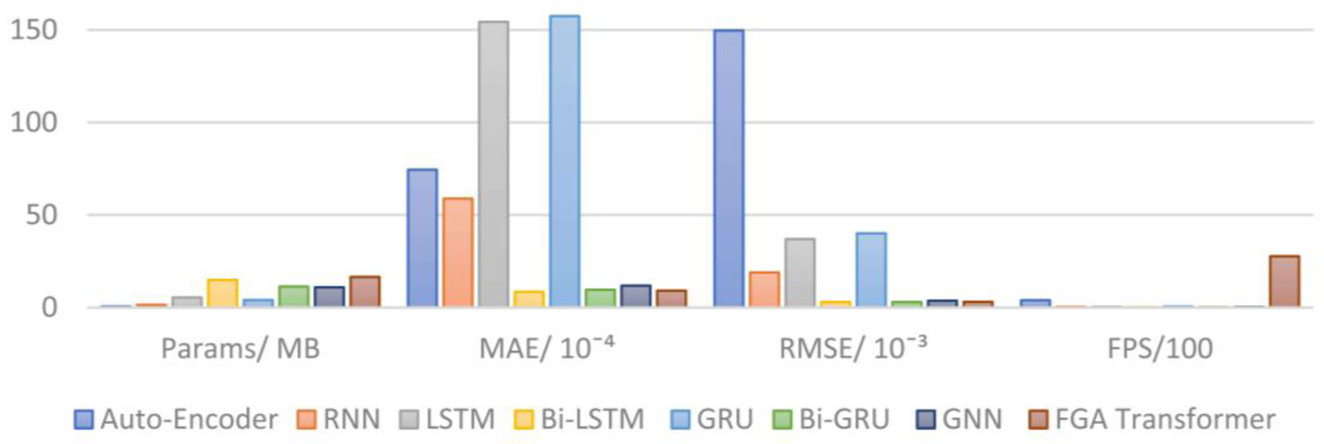
4.5. Comparison with Other Methods

We further investigate the capability of the FGA Transformer compared with other methods on various datasets [5,33,34]. For the auto-encoder [10], the hidden dimension is 256, the layer depth is 3, and the compressing rate is 0.6 for each layer. For RNN, LSTM [6], BiLSTM [7], GRU, and BiGRU [18], the hidden dimension is 256, and the layer depth is 3. For GNN [19], the number of layers is 3, the graph layer depth is 2, the number of neighbors is half the number of nodes, and the node dimension is 40. The dropout probability, input length, batch size, and learning rate for all the compared methods are set to 0.2, 128, 64 and $1\times {10}^{-4}$. The Adam optimizer and early stopping rule are used. These hyperparameters are detailed in

Table 10. Comparison methods and hyperparameters.

Model	Hyperparameters
Common Hyperparameters	dropout_prob = 0.2, input_length = 128, batch_size = 64, learning_rate = 1 × 10−4, optimizer = Adam
Auto-Encoder [10]	hidden_dim = 256, compression_rate = 0.6, layer_depth = 3
RNN	hidden_dim = 256, layer_depth = 3
LSTM [6]	hidden_dim = 256, layer_depth = 3
Bi-LSTM [7]	hidden_dim = 256, layer_depth = 3
GRU	hidden_dim = 256, layer_depth = 3
Bi-GRU [18]	hidden_dim = 256, layer_depth = 3
GNN [19]	stack_num = 4, graph_depth = 2, nodes_num = IDs_num, neighbors_num = int(IDs_num)/2, node_dim = 40, conv_channels = 16, residual_channels = 16

.

The comparison results, detailed in

Table 11. Comparison results on Car-Hacking dataset.

Model	Params/MB	MAE (Norm)/10−4	RMSE (Norm)/10−3	FPS
Auto-Encoder [10]	0.6	240.63	87.84	327.36
RNN	1.4	107.98	42.71	36.23
LSTM [6]	5.4	159.21	55.15	35.48
Bi-LSTM [7]	15.0	5.45	2.42	12.98
GRU	4.1	150.67	49.63	47.62
Bi-GRU [18]	11.3	5.22	2.21	17.81
GNN [19]	10.0	6.17	2.48	16.10
FGA Transformer	16.6	3.64	1.86	2178.35

,

Table 12. Comparison results on SynCAN bus dataset.

Model	Params/MB	MAE (Norm)/10−4	RMSE (Norm)/10−3	FPS
Auto-Encoder [10]	0.5	74.44	149.63	393.52
RNN	1.4	58.81	18.92	38.58
LSTM [6]	5.4	154.30	36.97	37.12
Bi-LSTM [7]	14.9	8.46	2.95	16.07
GRU	4.0	157.4	40.05	49.82
Bi-GRU [18]	11.3	9.59	2.93	18.49
GNN [19]	10.9	11.81	3.67	24.75
FGA Transformer	16.5	9.10	3.03	2768.30

and

Table 13. Comparison results on Automotive Sensor dataset.

Model	Params/MB	MAE/10−5	RMSE/10−5	FPS
Auto-Encoder [10]	0.5	18.94	65.69	335.98
RNN	1.3	51.43	178.16	37.72
LSTM [6]	5.3	27.87	96.55	36.22
Bi-LSTM [7]	14.9	27.37	94.81	15.61
GRU	4.0	5.58	18.87	48.62
Bi-GRU [18]	11.2	5.02	17.38	17.87
GNN [19]	9.0	4.61	15.98	49.75
FGA Transformer	16.4	9.84	30.66	3062.44

and illustrated in Figure 8, Figure 9 and Figure 10, provide a comprehensive overview of the performance of our proposed FGA Transformer against other state-of-the-art methods. Our FGA Transformer not only achieves a prediction accuracy that is comparable to its competitors but also demonstrates remarkable processing speeds. These speed advantages are primarily due to our adoption of a single-head attention mechanism and the fast approximation computation method. The single-head attention mechanism simplifies the architecture, reducing computational overhead, while the fast approximation technique accelerates the calculation process without sacrificing significant accuracy. Additionally, the spatiotemporal encoding mechanism allows the model to capture and utilize both temporal and spatial relationships within the CAN bus data, thereby improving the overall performance of the FGA Transformer in terms of prediction accuracy.

In the context of the Car-Hacking dataset, the FGA Transformer emerges as the leader in terms of both speed and accuracy metrics. This positions it as a suitable candidate for deployment on vehicle-end devices, where real-time processing capabilities are crucial. However, on the SynCAN dataset, the Bi-LSTM model outperforms our method, suggesting that for certain datasets, recurrent neural network architectures may be more appropriate. Similarly, on the Automotive Sensor dataset, methods such as GRU, BiGRU, and GNN show superior performance. It is important to note that these two datasets are characterized by lower data dimensions and stronger correlations, making them more amenable to simpler methods.

Our FGA Transformer can extract meaningful features from complex data, making it a robust choice for real-world CAN bus data. In terms of computational efficiency, our method consistently outperforms the competition across all three datasets, highlighting its advantage in scenarios where rapid data processing is paramount.

The underwhelming prediction performance of the auto-encoder can be attributed to its aggressive dimensionality reduction, which may result in the loss of critical information. Additionally, recurrent models like RNN, LSTM, and GRU face challenges in handling irregular time intervals and do not show a clear advantage in terms of accuracy or speed when dealing with CAN bus data. These limitations hinder the broader application of these methods, particularly in contexts where both accuracy and speed are essential.

Despite the FGA Transformer’s robust performance on complex CAN bus datasets, it may not always outperform other methods, particularly on simpler data. This discrepancy can be attributed to the inherent complexity of CAN bus data, which our model is specifically designed to handle. The model faces challenges in predicting infrequently occurring CAN IDs. Although our data cleaning process partly contributes to this issue by removing infrequent data, it also highlights a broader challenge in learning from extremely imbalanced datasets. Even if we were to keep these rare CAN IDs, the network would struggle to learn their characteristics from sliced data segments, as they are overwhelmed by the more prevalent data points. Moreover, the computational requirements of capturing these rare events in longer data segments are impractical, particularly at the segment edges, which is not feasible in practice. Additionally, the sensitive nature of CAN bus data often precludes cloud processing, necessitating local solutions with limited computational resources.

In summary, while the FGA Transformer may not outperform other methods in every scenario, its overall performance, especially in terms of processing speed and accuracy on complex datasets, makes it a compelling choice for CAN bus data analysis.

5. Application of the FGA Transformer in Practical Scenarios

This section discusses the practical applications of the FGA Transformer in automotive scenarios. Two feasible approaches are presented:

The first approach involves deploying an edge device, which listens to data from the OBD interface. The FGA Transformer is then utilized to analyze and predict the vehicle data. By analyzing the vehicle data, abnormal thresholds can be set, and alerts can be provided to the user. This method can detect vehicle damage or attacks without requiring high levels of vehicle intelligence. The modification cost is relatively low. However, the primary challenges may lie in the edge device’s insufficient computing power to support more complex algorithms and its difficulty in processing longer data segments. A promising solution to address the challenge is to adopt model compression techniques such as distillation. This method can significantly enhance the inference speed of the FGA Transformer at the edge, while still maintaining its predictive capabilities.

The second approach involves deploying the FGA Transformer into the computing core of an intelligent vehicle. It is also possible to use the vehicle’s normal driving data for continuous training and model improvement. By using Federated Learning, the model can be updated in the cloud and then distributed to users. This method has higher performance requirements for the vehicle. However, if the vehicle meets these requirements, manufacturers can use Over-the-Air (OTA) technology to continuously improve the user experience. A potential challenge in this approach is the secure transmission of data. To overcome this challenge, we propose the implementation of robust encryption and authentication mechanisms.

Overall, the two implementation approaches are not only applicable to the FGA Transformer but also to other unsupervised vehicle CAN bus data analysis methods.

6. Conclusions

In this paper, we have presented a novel Transformer architecture named FGA Transformer, aimed at learning and predicting CAN bus data under the constraints of limited computing resources on the vehicle side. The core design of the FGA Transformer is the fast-gated attention mechanism. By splitting the sensors into parallel groups, employing gated attention instead of multi-head attention, and using the FAVOR+ approach, this fast attention mechanism fully extracts spatiotemporal features of time series data. The max pooling cross-window can enlarge the attention area of each Transformer layer efficiently.

We have compared our method with numerous time series prediction methods on three diverse datasets: Car-Hacking [33], SynCAN [34], and Automotive Sensors [5]. Our FGA Transformer method achieved RMSE prediction errors of $1.86\times {10}^{-3}$, $3.03\times {10}^{-3}$, and $30.66\times {10}^{-3}$ and MAE errors of $3.64\times {10}^{-4}$, $9.1\times {10}^{-4}$, and $9.84\times {10}^{-5}$, respectively, which are the best or comparable to the highest prediction accuracies among the compared methods. In terms of inference speed, our method outperforms the others by one to two orders of magnitude, with speeds of 2178, 2768, and 3062 FPS, respectively. This significant advantage is primarily due to the max pooling cross-window technique, which ensures the precision of spatiotemporal feature extraction, and the fast-gated attention mechanism, which greatly accelerates inference speed through rapid approximate computations of the gated single-head attention mechanism.

Lastly, we have outlined two implementation strategies for real-world scenarios, which have the potential to significantly advance the automotive industry by enabling more sophisticated anomaly detection and prediction capabilities in vehicle CAN bus systems. This advancement could lead to improved vehicle safety, enhanced driving experiences, and more efficient maintenance strategies.

Our FGA Transformer has successfully extracted hidden association features between different CAN IDs. However, these features are not explicitly extractable, which limits the interpretability of the network and its applicability across different vehicle brands. In our future work, we aim to address this by integrating graph neural network (GNN) methods. We plan to represent each CAN ID as a node in a graph, with an adjacency matrix describing the relationships between the CAN devices. This adjacency matrix will be learned from the data, allowing us to propagate the influence of each node. This approach aims to achieve improved performance and provide the potential for manual network adjustment.

References

1. Luo, Y.; Xiao, Y.; Cheng, L.; Peng, G.; Yao, D. Deep learning-based anomaly detection in cyber-physical systems: Progress and opportunities. ACM Comput. Surv. 2021, 54, 1–36. [Google Scholar] [CrossRef]
2. Martinez, C.M.; Heucke, M.; Wang, F.Y.; Gao, B.; Cao, D. Driving style recognition for intelligent vehicle control and advanced driver assistance: A survey. IEEE Trans. Intell. Transp. Syst. 2017, 19, 666–676. [Google Scholar] [CrossRef]
3. Wang, C.; Xu, X.; Xiao, K.; He, Y.; Yang, H.; Yang, G. Traffic anomaly detection algorithm for CAN bus using similarity analysis. High-Confid. Comput. 2024, 9, 14–21. [Google Scholar] [CrossRef]
4. He, T.; Zhang, L.; Kong, F.; Salekin, A. Exploring inherent sensor redundancy for automotive anomaly detection. In Proceedings of the ACM/IEEE Design Automation Conference, San Francisco, CA, USA, 20–24 July 2020; pp. 1–6. [Google Scholar]
5. Hanselmann, M.; Strauss, T.; Dormann, K.; Ulmer, H. CANet: An unsupervised intrusion detection system for high dimensional CAN bus data. IEEE Access 2020, 8, 58194–58205. [Google Scholar] [CrossRef]
6. Qin, H.; Yan, M.; Ji, H. Application of controller area network (CAN) bus anomaly detection based on time series prediction. Veh. Commun. 2021, 27, 100291. [Google Scholar] [CrossRef]
7. Sun, H.; Chen, M.; Weng, J.; Liu, Z.; Geng, G. Anomaly detection for in-vehicle network using CNN-LSTM with attention mechanism. IEEE Trans. Veh. Technol. 2021, 70, 10880–10893. [Google Scholar] [CrossRef]
8. Kishore, C.R.; Rao, D.C.; Nayak, J.; Behera, H.S. Intelligent intrusion detection framework for anomaly-based can bus network using bidirectional long short-term memory. J. Inst. Eng. India Ser. B 2024, 105, 541–564. [Google Scholar] [CrossRef]
9. Song, H.M.; Kim, H.K. Self-supervised anomaly detection for in-vehicle network using noised pseudo normal data. IEEE Trans. Veh. Technol. 2021, 70, 1098–1108. [Google Scholar] [CrossRef]
10. Narasimhan, H.; Ravi, V.; Mohammad, N. Unsupervised deep learning approach for in-vehicle intrusion detection system. IEEE Consum. Electr. Mag. 2021, 12, 103–108. [Google Scholar] [CrossRef]
11. Agrawal, K.; Alladi, T.; Agrawal, A.; Chamola, V.; Benslimane, A. NovelADS: A novel anomaly detection system for intra-vehicular networks. IEEE Trans. Intell. Transp. Syst. Mag. 2022, 23, 22596–22606. [Google Scholar] [CrossRef]
12. Koltai, B.; Gazdag, A.; Acs, G. Supporting CAN bus anomaly detection with correlation data. In Proceedings of the International Conference on Information Systems Security and Privacy, Rome, Italy, 26–28 February 2024; pp. 285–296. [Google Scholar]
13. Wei, P.; Wang, B.; Dai, X.; Li, L.; He, F. A novel intrusion detection model for the CAN bus packet of in-vehicle network based on attention mechanism and autoencoder. Digit. Commun. Netw. 2023, 9, 14–21. [Google Scholar] [CrossRef]
14. Song, H.M.; Woo, J.; Kim, H.K. In-vehicle network intrusion detection using deep convolutional neural network. Veh. Commun. 2020, 21, 100198. [Google Scholar] [CrossRef]
15. Ning, J.; Wang, J.; Liu, J.; Kato, N. Attacker identification and intrusion detection for in-vehicle networks. IEEE Commun. Lett. 2019, 23, 1927–1930. [Google Scholar] [CrossRef]
16. Duan, X.; Yan, H.; Tian, D.; Zhou, J.; Su, J.; Hao, W. In-vehicle CAN bus tampering attacks detection for connected and autonomous vehicles using an improved isolation forest method. IEEE Trans. Intell. Transp. Syst. 2023, 24, 2122–2134. [Google Scholar] [CrossRef]
17. Zhao, X.; Han, X.; Su, W.; Yan, Z. Time series prediction method based on Convolutional Autoencoder and LSTM. In Proceedings of the Chinese Automation Congress, Hangzhou, China, 22–24 November 2019; pp. 5790–5793. [Google Scholar]
18. Zhang, Y.; Thorburn, P.J. A dual-head attention model for time series data imputation. Comput. Electron. Agric. 2021, 189, 106377. [Google Scholar] [CrossRef]
19. He, Z.; Zhao, C.; Huang, Y. Multivariate Time Series Deep Spatiotemporal Forecasting with Graph Neural Network. Appl. Sci. 2022, 12, 5731. [Google Scholar] [CrossRef]
20. Fan, J.; Zhang, K.; Huang, Y.; Zhu, Y.; Chen, B. Parallel spatio-temporal attention-based TCN for multivariate time series prediction. Neural Comput. Appl. 2023, 35, 13109–13118. [Google Scholar] [CrossRef]
21. Wang, H.; Zhang, Y.; Liang, J.; Liu, L. DAFA-BiLSTM: Deep autoregression feature augmented bidirectional LSTM network for time series prediction. Neural Netw. 2023, 157, 240–256. [Google Scholar] [CrossRef]
22. Gao, Z.; Kuruoğlu, E.E. Attention based hybrid parametric and neural network models for non-stationary time series prediction. Expert Syst. 2024, 41, 13419. [Google Scholar] [CrossRef]
23. Bono, F.M.; Radicioni, L.; Cinquemani, S. A novel approach for quality control of automated production lines working under highly inconsistent conditions. Eng. Appl. Artif. Intell. 2023, 122, 106149. [Google Scholar] [CrossRef]
24. Chen, Y.; Ding, F.; Zhai, L. Multi-scale temporal features extraction based graph convolutional network with attention for multivariate time series prediction. Expert Syst. Appl. 2022, 200, 117011. [Google Scholar] [CrossRef]
25. Buscemi, A.; Turcanu, I.; Castignani, G.; Crunelle, R.; Engel, T. CANMatch: A Fully Automated Tool for CAN Bus Reverse Engineering based on Frame Matching. IEEE Trans. Veh. Technol. 2021, 70, 12358–12373. [Google Scholar] [CrossRef]
26. Wen, H.; Zhao, Q.; Chen, Q.A.; Lin, Z. Automated cross-platform reverse engineering of CAN bus commands from mobile apps. In Proceedings of the Network and Distributed System Security Symposium, San Diego, CA, USA, 23–26 February 2020; pp. 3–17. [Google Scholar]
27. Guyon, I.; Luxburg, U.V.; Bengio, S.; Wallach, H.; Fergus, R.; Vishwanathan, S.; Garnett, R. Attention is all you need. In Proceedings of the 31st Conference on Neural Information Processing Systems, Long Beach, CA, USA, 4–9 December 2017; pp. 5998–6008. [Google Scholar]
28. Ho, J.; Kalchbrenner, N.; Weissenborn, D.; Salimans, T. Axial Attention in Multidimensional transformers. arXiv 2019, arXiv:1912.12180. [Google Scholar]
29. Huang, Z.; Wang, X.; Huang, L.; Huang, C.; Wei, Y.; Liu, W. Ccnet: Criss-cross attention for semantic segmentation. In Proceedings of the IEEE/CVF International Conference on Computer Vision, Seoul, Republic of Korea, 27 October–2 November 2019; pp. 603–612. [Google Scholar]
30. Dong, X.; Bao, J.; Chen, D.; Zhang, W.; Yu, N.; Yuan, L.; Chen, D.; Guo, B. Cswin transformer: A general vision transformer backbone with cross-shaped windows. In Proceedings of the IEEE/CVF Conference on Computer Vision and Pattern Recognition, New Orleans, LA, USA, 21–24 June 2022; pp. 12124–12134. [Google Scholar]
31. Hua, W.; Dai, Z.; Liu, H.; Le, Q. Transformer quality in linear time. In Proceedings of the International Conference on Machine Learning, Baltimore, MD, USA, 17–23 July 2022; pp. 9099–9117. [Google Scholar]
32. Choromanski, K.; Likhosherstov, V.; Dohan, D.; Song, X.; Gane, A.; Sarlos, T.; Hawkins, P.; Davis, J.; Mohiuddin, A.; Kaiser, L.; et al. Rethinking attention with performers. arXiv 2020, arXiv:2009.14794. [Google Scholar]
33. Song, H.M.; Kim, H.K. Can Network Intrusion Datasets. 2018. Available online: http://ocslab.hksecurity.net/Datasets/car-hacking-dataset (accessed on 28 August 2018).
34. Stocker, A.; Kaiser, C.; Festl, A. Automotive Sensor Data. An Example Dataset from the AEGIS Big Data Project. 2017. Available online: https://zenodo.org/records/820576 (accessed on 28 June 2017).
Figure 1. Format of the CAN bus frame.
Electronics 13 02707 g001
Figure 2. (Left): the overall architecture of our proposed FGA Transformer. (Right): an illustration of the FGA Transformer block.
Electronics 13 02707 g002
Figure 3. Illustration of self-attention mechanisms.
Electronics 13 02707 g003
Figure 4. Impact of pre-processing methods.
Electronics 13 02707 g004
Figure 5. Impact of various attention mechanisms.
Electronics 13 02707 g005
Figure 6. Impact of various attention windows.
Electronics 13 02707 g006
Figure 7. Impact of group size.
Electronics 13 02707 g007
Figure 8. Comparison results on Car-Hacking dataset.
Electronics 13 02707 g008
Figure 9. Comparison results on SynCAN bus dataset.
Electronics 13 02707 g009
Figure 10. Comparison results on Automotive Sensor dataset.
Electronics 13 02707 g010