Abstract
A significant challenge encountered in mmWave and sub-terahertz systems used in 5G and the upcoming 6G networks is the rapid fluctuation in signal quality across various beam directions. Extremely high-frequency waves are highly vulnerable to obstruction, making even slight adjustments in device orientation or the presence of blockers capable of causing substantial fluctuations in link quality along a designated path. This issue poses a major obstacle because numerous applications with low-latency requirements necessitate the precise forecasting of network quality from many directions and cells. The method proposed in this research demonstrates an avant-garde approach for assessing the quality of multi-directional connections in mmWave systems by utilizing the Liquid Time-Constant network (LTC) instead of the conventionally used Long Short-Term Memory (LSTM) technique. The method’s validity was tested through an optimistic simulation involving monitoring multi-cell connections at 28 GHz in a scenario where humans and various obstructions were moving arbitrarily. The results with LTC are significantly better than those obtained by conventional approaches such as LSTM. The latter resulted in a test Root Mean Squared Error (RMSE) of 3.44 dB, while the former, 0.25 dB, demonstrating a 13-fold improvement. For better interpretability and to illustrate the complexity of prediction, an approximate mathematical expression is also fitted to the simulated signal data using Symbolic Regression.
1. Introduction
Wireless communication systems, particularly the 5G and the upcoming 6G networks, are increasingly adopting the extremely high-frequency (EHF) millimeter-wave (mmWave) and tremendously high-frequency (THF) sub-terahertz T-waves. The wavelength of the mmWave frequencies is between one centimeter and one millimeter, hence the name. They offer a large amount of available spectrum, greater capacity, and more bandwidth than traditional bands. This means that they can be used to provide very high data rates. The 5G and 6G wave technology for mobile network operators enable many important applications such as autonomous driving [1], precision agriculture [2], mobile virtual reality [3], and high-definition video broadcasting [4]. They offer faster deployment and higher return on investment (ROI). Multi-link prediction refers to the process of forecasting the quality of potential connections between a user device and a base station. Unlike traditional cellular networks where there is a single connection between a device and a tower, mmWaves use narrow, steerable beams and follow a process called beamforming. Therefore, connections along multiple paths can be formed simultaneously. The quality of the connection is often measured by the Signal-to-Noise Ratio (SNR). Higher values indicate a stronger signal relative to background noise. By predicting the quality, the device can seamlessly switch to the predicted high-quality link without losing the connection.
However, owing to their short wavelength, EHF and THF waves have a strict Line of Sight requirement. This means that they cannot travel through walls or trees and are highly sensitive to obstacles. The channel changes very quickly as the user moves. Wireless systems using them are impacted by fluctuating channel quality when the beam propagates in various directions simultaneously. Millimeter-wave communication is also not energy efficient. Slight deviations in the path of the transceivers or the presence of interfering elements can cause significant alterations in link quality unpredictably. Low-latency applications necessitate the ability to accurately forecast the link quality across different cells and directions. Previous attempts to address the challenge of predicting multiple links using AI/ML techniques involved certain Recurrent Neural Network (RNN) models like Long short-term memory (LSTM) for the link prediction [5].
Link prediction is the important task of estimating the quality of the signal between nodes in a network. It plays an important role in EHF and THF systems because these signals are inherently flaky and unpredictable, but the low-latency applications require accurate prediction. Link prediction helps in optimizing network performance, making routing decisions, and resource allocation.
Traditionally, the parameters for Artificial Neural Networks (ANNs), including RNNs like LSTM are fixed after training. ANNs use these fixed parameters to make decisions, a process called inferencing. Liquid Neural Networks (LNNs) are a better type of RNN that can learn even at the time of decision-making and are therefore better suited to real-world applications [6]. LNNs are a progression of Neural Ordinary Differential Equations (ODEs). Neural ODEs [7] use an approximation to evolve the hidden state by using a fixed time interval or a “time constant”. Liquid Time-Constant Networks or LTCs are a special type of LNN that use a time constant that is not fixed, giving it the flexibility to dynamically adapt to changes in the data [8], which for this work is the wireless EHF and THF signal. We hypothesize that LTCs are better suited to the problem of multi-link prediction for mmWave and sub-terahertz because of the highly unpredictable nature of the signal, and the experiments detailed later confirm this. LTCs adapt to the rapid fluctuations in the data even during inferencing [9]. Their behavior is more explainable, they can learn from smaller amounts of data, and are computationally effective, requiring a smaller number of neurons [8]; hence, they can run on edge devices like smartphones.
The simulation in this work is based on the Urban Microcellular Infrastructure (UMI) Channel model [10], an indoor scenario that typically uses 28 GHz as the operating carrier frequency. Therefore, the EHF and THF waves are generated for the experimental setup using a real-time simulation involving multiple links with trajectories of moving individuals and obstructing vehicles in a scenario set at 28 GHz. The simulation uses appropriate noise figure and path loss encompassing both Line-of-Sight (LOS) and Non-Line-of-Sight (NLoS) propagation paths following the 3GPP Channel model [11]. The parameters set for the simulation are as specified in Table 1. Also, the current literature [5] uses 28 GHz for experiments with LSTM. Using the same 28 GHz frequency for this work helps ensure a fair evaluation of the results.

Table 1.
NYUSIM simulation parameters for generating the data.
The experiments hypothesize that more precise and reliable predictions regarding the link quality in complex wireless communication scenarios can be achieved using LTCs. The proposed LTC-based Multi-Link Prediction model seeks to enhance the accuracy and efficiency of link quality predictions by leveraging recent developments in artificial intelligence technologies. The experiments are intended to validate the effectiveness of LTCs in a practical simulation environment to confirm the hypothesis that LTCs address the challenges associated with predicting link quality in dynamic wireless communication systems. This research contributes to the evolution of predictive modeling in wireless communication, paving the way for robust and adaptive systems in the future as wireless communication systems evolve towards 6G networks and beyond.
In the case of mmWave frequencies, it is expected that the distance between cellular base stations remains consistent. With carrier frequencies progressing towards terahertz, the wider bandwidth of the channel allows for covering similar distances. This is achieved through the exponential growth in antenna gains as frequencies rise, assuming the physical antenna remains unchanged [12].
The LSTM model is impacted by certain shortcomings when used for link prediction for EHF and THF. LSTM outcomes tend to be less accurate, particularly in scenarios where prediction involves data that are not continuous. EHF and THF waves are prone to attenuation due to the oxygen and other matter in the atmosphere. The waves are absorbed by certain compounds such as water vapor in the atmosphere. The higher the frequency, the greater the absorption. Also, as mentioned earlier, EHF and THF waves propagate only along the Line-of-Sight paths. They cannot bend around obstacles. Due to the varying distances between the transmitter, receiver, and any obstructing objects present on each link, the signal could be choppy. Consequently, for such scenarios, when the LSTM model is applied, the results may not be accurate to the desired extent. In scenarios where there are more links between the transmitter and the receiver, the effectiveness of an LSTM model might diminish, resulting in suboptimal predictions [13,14].
The overall mobile handover operation (HO) probability with respect to both horizontal as well as vertical hand-off needs to be characterized to attain specific mobile coverage probability in mmWave and sub-terahertz networks [15].
1.1. Related Work
A combination of Convolutional Neural Network (CNN) and Recurrent Neural Network (RNN) deep learning models have been used to predict future blockages and beams for mmWave systems. This helps with proactive handovers between base stations to ensure uninterrupted connectivity for users [16]. Diverse approaches have been tried for link quality prediction, including using camera images [17]. Predicting link blockages is important to ensure seamless connectivity. The predictions help to proactively switch beams and handoff (HO). Computer vision has been used to conduct these predictions based on camera images in yet another work [18]. Transfer learning using deep neural networks was attempted to predict the optimal beams for multi-links, resulting in reduced interference and training overhead [19]. EHF waves suffer from low spectral efficiency, narrow coverage, and difficulty in Non-Line-of-Sight (NLoS) propagation. It is therefore important to model path loss accurately for optimal base station placement. There are three types of path loss modeling methods: empirical, deterministic, and machine learning-based. Machine learning-based modeling uses measured data to train a model to predict path loss. A novel machine learning scheme called multi-way local attentive learning has been proposed to model and predict path loss [20].
By understanding the environment using a combination of analytical models such as geometric analysis to recognize the shadowed regions that separate Line-of-Sight (LoS) and Non-Line-of-Sight (NLoS) scenarios and deep neural networks, researchers have built systems that can proactively allocate resources for better performance [21]. The allocation is based on link quality predictions as described in this work but using deep neural networks for regression. Not just deep learning, but traditional machine learning techniques such as Support Vector Regression (SVR), Random Forest (RF), and Gradient Tree Boosting (GTB) have also been used for the task of mmWave link prediction [22]. In yet another novel approach, researchers extract a sparse feature representation using non-deterministic quantization and apply deep neural network (DNN) to learn from those features for mmWave beam prediction [23]. Channel State Information (CSI) is fused with information about the user’s location to predict the beam [24]. The prediction is still carried out using a neural network that adopts Adjustable Feature Fusion Learning (AFFL).
Another approach [25] combines Deep Neural Networks (DNNs) with Long Short-Term Memory (LSTM) networks to create a new prediction method. This approach considers both past channel information and the position of the device. The proposed method can predict both large-scale trends and small-scale fluctuations in mmWave channel features. The approach achieved over 4.5% improvement in accuracy compared to existing approaches. To detect the motion of blockers such as a walking person close to the Line-of-Sight (LoS) path, an mmAlert system was proposed [26] using the passive sensing technique. It could predict 90% of the LoS blockage, with a sensing time of 1.4 s being sufficient enough to provide a timely warning. Privacy is important in such applications. To preserve privacy, instead of cameras, point clouds have been used for predicting signal strength in millimeter-wave communication systems [27]. Point clouds are 3D representations of spaces. While cameras may capture sensitive information, point clouds are devoid of privacy concerns. The approach still achieves accuracy that is comparable to traditional image-based methods.
As can be seen, link prediction has been attempted via several methods, mostly using deep learning through Artificial Neural Networks (ANN) and some traditional machine learning approaches. The accuracy of the prediction is reasonable but, as this work confirms, LTC predictions are far more accurate than with LSTM, which so far was the most relevant deep learning framework for the problem.
1.2. Contribution
To our knowledge, this work is unique in achieving a significantly better prediction of the Signal-to-Noise Ratio (SNR) of EHF signals using Liquid Time-Constant Networks. Explainability and interpretability play an important role in machine learning [28]. This work is also novel in applying Symbolic Regression to fit a mathematical expression to SNR values of a simulated EHF wireless system for interoperability. The core research contributions can be summarized as follows:
- Quantitative demonstration of substantial improvement in multi-link prediction for mmWave wireless communication systems using Liquid Time-Constant Networks (LTC) over conventional methods such as using Long Short-Term Memory.
- Interpretation of the SNR values of mmWave signal using Symbolic Regression.
The rest of the paper is organized as follows. Section 2 details the approach followed for the experiments. It briefly explains the concepts, the dataset used, how it was generated, and the setup for Symbolic Regression. Numerical experiments, including the hyperparameter settings, and results are discussed in Section 3. Section 4 discusses the results from the experiments and the conclusions are included in Section 5.
2. Materials and Methods
For simulating the mmWave and sub-terahertz wireless channels, an open-source simulator developed by the New York University called NYUSIM is used. The product can simulate many real-life environments such as urban macrocell, urban microcell, indoor hotspot, and rural macrocell. The performance of a simulated communication channel is measured by the Signal-to-Noise Ratio (SNR). The SNR is a measure of the quality of the received signal and is defined as the ratio of the power of the received signal to the power of the noise present in the channel [29]. The data generated using the simulator are then used for the experiments with LSTM and LTC. The results from both are compared to test the hypothesis that LTC achieves better prediction. A mathematical expression is also fitted to the data using Symbolic Regression through genetic programming [30]. The mathematical expression gives insights into the nature of variations in the SNR values.
2.1. Long Short-Term Memory—LSTM
For comparison, the results from using LSTM [31] for link quality prediction are used as the baseline. The training part is performed using a dataset that has Signal-to-Noise (SNR) values generated during simulation trials, enabling the model to decrypt the underlying patterns and links. The input layer of the LSTM network takes the SNR value sequence, followed by a hidden layer, and then an output layer. The LSTM cells in the model function in a unidirectional manner, aiding in the sequential processing of data. The training of the model utilizes back-propagation through time, which efficiently propagates error gradients through the LSTM cells over temporal spans. The results highlight the effectiveness and assurance of LSTM models in tasks associated with the prediction of new SNR values as the signal propagates.
2.2. LTC
The experiments are then repeated using LTC instead of LSTM. The SNR values are now passed as inputs to LTC. LTCs are also a type of Recurrent Neural Networks (RNN). Unlike the traditional RNNs, which process information in discrete steps, LTC networks handle information that is more unpredictable over time. Mathematically, they operate using differential equations, allowing them to model systems that evolve more dynamically [8]. A key feature of LTC is the concept of a “liquid time constant”, from which LTC gets its name. This refers to the fact that each neuron in the network has its internal timescale for processing information. This flexibility allows the network to capture more granular rates of change in the data even at the time of inferencing.
2.3. Dataset: Simulation
The dataset comprises Signal-to-Noise Ratio (SNR) measurements calculated every 20 ms. SNR is computed by comparing the received signal power to the noise power in the channel. The efficiency of a telecommunications system model operating in an urban microcell indoor environment was examined in this work. A frequency of 28 GHz was used to generate the SNR values in the dataset. The parameters for the environment setup used for the simulation are as shown in Table 1. The parameters are self-explanatory.
The large-scale path loss model used in NYUSIM is a Close-In free space reference distance (CI) model with a 1 m reference distance [32]. It includes an extra attenuation term due to various atmospheric conditions. The model is given by Equation (1).
where is the path loss in dB at a distance of d meters and carrier frequency of f GHz;
- is the free space path loss in dB at a distance of 1 m and carrier frequency of f GHz;
- n is the path loss exponent (n = 2 for free space);
- is the total atmospheric absorption term;
- is the shadow fading (SF) that refers to the signal attenuation due to obstacles in the Line of Sight, modeled as a log-normal random variable with zero mean;
- is the standard deviation in dB.
The Free Space Path Loss (FSPL), an idealized theoretical concept that refers to the attenuation of radio signal strength as it travels through space, with no obstacles or reflections, is given by Equation (2).
where c is the speed of light.
The path loss exponent is a parameter that describes how the path loss increases with distance. For free space, the path loss exponent is 2. However, the path loss exponent can vary depending on the environment. For example, in urban areas, the path loss exponent is typically greater than 2 due to the presence of buildings and other obstructions. The total atmospheric absorption term is a measure of the attenuation of the signal due to absorption by the atmosphere. The absorption is caused by the interaction of the radio waves with the molecules in the atmosphere. The absorption is frequency-dependent, with higher frequencies being absorbed more than lower frequencies [33].
Shadow fading is a random variation in the received signal strength due to changes in the propagation environment. Shadow fading is caused by changes in the terrain, buildings, and other objects between the transmitter and receiver. Shadow fading is typically modeled as a log-normal random variable [29] as can be seen from Equation (1).
The large-scale path loss model is used to predict the received signal strength at a given distance from the transmitter. The model can be used to design wireless networks and to estimate the coverage area of a wireless network [33].
2.4. Dataset Generation
The program to generate the dataset of SNR values using the simulator is written in MATLAB R2022b Update 9 (9.13.0.2553342), 64-bit (maci64). The SNR values are produced by simulating an mmWave wireless communication system operating at a carrier frequency of 28 GHz, encompassing both Line-of-Sight (LOS) and Non-Line-of-Sight (NLoS) propagation paths. The procedure emulates a Channel Impulse Response (CIR) for each trajectory, followed by multiplication with a random input signal to produce a received signal. The SNR is calculated as the ratio of signal power to noise power, assuming noise power is directly proportional to signal power, and a fixed SNR of 30 dB is maintained.
2.5. SNR Calculation
There are several imperative tools used for classifying the various patterns of mobility in wireless communications. These patterns are known as mobility models and include the Vehicular Mobility Model, the High-Speed Train Mobility Model, the Human Mobility Model, and the Ship Mobility Model. Through the extraction of extensive datasets, such mobility models provide researchers with the ability to scrutinize and approximate the influence of several mobility factors such as vehicular speed, congestion levels, ambiguity, social interactions, location preferences, and more. To perform an extensive experiment in this field, it is critically important to assess both the Human Mobility Model (HMM) and the Vehicular Mobility Model (VMM) as they play a vital role in apprehending and speculating the dynamics of wireless communications. By concentrating on such specific mobility models, researchers can attain valuable insights into the complexities of mobility patterns and enhance the overall efficiency and reliability of wireless communication systems [5].
Using a simulated channel model, an assessment has been conducted to determine the received signal power and noise power at the user equipment. The received signal power is calculated as the product of the transmitted power, the antenna gain, and the path loss between the base station and the User Equipment (UE). The noise power is calculated as the product of the noise figure, the bandwidth, and the Boltzmann constant. Then, the Signal-to-Noise Ratio (SNR) is calculated as the ratio of the power of the received signal to the power of the noise, expressed in decibels (dB) [34].
The Signal-to-Noise Ratio (SNR) is calculated as the ratio of the power of the received signal to the power of the noise, expressed in decibels (dB). In the context of this problem, the SNR can be calculated as
where is the power of the received signal and is the power of the noise.
The parameters required to calculate the SNR for this problem are as follows. : The power of the received signal, which is calculated as the product of the channel gain and the transmitted power. : The power of the noise, which is calculated as the product of the noise figure and the receiver bandwidth [5].
The distance between the transmitter and receiver, the carrier frequency, and the properties of the propagation environment determine the channel gain. The transmitter power and receiver bandwidth are also specified in the problem. The noise figure represents the noise added by the receiver and is also specified in the problem [5].
Subsequently, an analysis has been conducted to establish the SNR by comparing the power of the received signal to the power of the noise, resulting in creating a dataset comprising SNR values recorded at 20 millisecond intervals. These recorded SNR values offer significant insights into the operational efficiency of the communication system within an indoor microcellular setting in urban areas [33].
2.6. Genetic Programming Based Symbolic Regression
The dataset is modeled using a mathematical expression to gain deeper insights into the SNR values generated and predict future SNR values using the mathematical expression. To find a mathematical expression that best fits a given dataset, Symbolic Regression is applied to the dataset. It is a type of regression analysis in which the goal is to find a mathematical expression that best fits a given set of data points. In contrast to traditional regression methods that use predefined functions such as linear or polynomial equations, Symbolic Regression allows the model to discover its own functional form by searching through a space of mathematical expressions. Genetic programming is a type of evolutionary algorithm that is used to find solutions to complex problems by mimicking the process of natural selection. In genetic programming, a population of candidate solutions, known as “individuals” is evolved over multiple generations using principles of genetic variation and selection. The fitness function is a measure of how well a particular individual—a potential solution—fits the data.
In Symbolic Regression, the fitness function is typically based on the degree of error between the actual data points and the predicted values generated by the individual’s mathematical expression. Crossover and mutation are two key genetic operators used in genetic programming. Crossover involves combining genetic material from two parent individuals to create a new offspring individual, while mutation involves randomly altering the genetic material of an individual in order to introduce new variations. Tournament selection is a common method of selecting individuals for reproduction in genetic programming. In tournament selection, a subset of individuals from the population is chosen at random, and the individual with the highest fitness within that subset is selected for reproduction. In genetic programming, individuals are represented as trees of nodes. Terminal nodes represent input variables or constants, while non-terminal nodes represent mathematical operations or functions [35].
The above experiment has been performed on the dataset that was generated by an earlier-simulated model consisting of SNR values. There are predefined arithmetic functions such as add, sub, mul sin, cos, etc., for the Symbolic Regression. The code is implemented in Python. The SymbolicRegressor class is imported from gplearn.genetic package. Custom-defined functions such as ReLU were defined and added to the function set to provide the algorithm with more flexibility in modeling the data. This can be achieved using the make_function() method. The other parameters that the SymbolicRegressor constructor can take to configure the model are as follows:
- population_size: The number of individuals (mathematical expressions) in each generation.
- function_set: The set of functions and terminals that can be used in the mathematical expressions.
- generations: The maximum number of generations to evolve the population.
- stopping_criteria: The threshold value for the Mean Absolute Error (MAE) to stop evolution if it falls below this value.
- p_crossover, p_subtree_mutation, p_hoist_mutation, p_point_mutation: The probabilities of applying crossover, subtree mutation, hoist mutation, and point mutation operations during evolution.
- max_samples: The maximum proportion of samples to use in each generation during fitness evaluation.
- verbose: Whether to enable verbose output during evolution.
- parsimony_coefficient: A coefficient to balance between the goodness of fit and the complexity (parsimony) of the mathematical expressions.
- random_state: The random seed for reproducibility.
These parameters allow us to customize the SymbolicRegressor model to fit the specific needs. For example, one can increase the population_size to improve the accuracy of the model, or these values could also be reduced generations to speed up the training process. After passing the dataset through the Symbolic Regressor, the symbolic expression obtained for the dataset is as follows.
Also, the above expression can be depicted as a tree diagram using the graphviz python package as shown in Figure 1. Graphviz helps visualize the complex math expressions discovered by Symbolic Regression as tree diagrams, making them easier to understand and analyze. The leaves of the math parse tree [36] are numeric constants and variables from the symbolic expression. The internal nodes of the tree are arithmetic operations such as addition, subtraction, multiplication, division, and sine. Traversing the tree to its root will generate the entire symbolic expression. The tree diagram is a visual indication of the complexity of the regression.
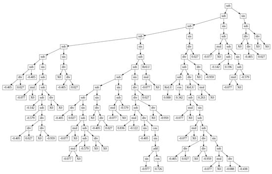
Figure 1.
The mathematical expression from the Symbolic Regression. Modeling the SNR values is depicted as a tree diagram for better visualization.
Now, when the trained model is evaluated for Symbolic Regression, the fit of the model to the data is determined by R2 score. R2 score is also called as the coefficient of determination. It is a statistical measure that tells how well a regression model, in this case the mathematical expression, fits the available data. It quantifies the proportion of variance in the dependent variable, the SNR values in this case, that is explained by the model. It ranges from 0 to 1, with 0 being the worst fit and 1 being the perfect fit. A higher R2 score means that the model is better at predicting the dependent variable. The evaluation of the model is illustrated in a scatter plot shown in Figure 2. The x-axis is the timeline indexed by the observation count. The y-axis refers to the Signal-to-Noise Ratio (SNR). The blue dotted line represents the observed SNR values. The red dotted line represents the symbolic function, which is the mathematical formula discovered by the Symbolic Regression algorithm to approximate the true function. The closer the red line is to the blue line, the better the fit.
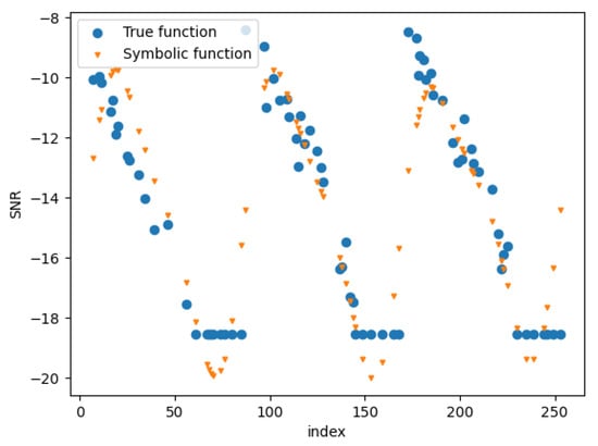
Figure 2.
The scatter plot from the Symbolic Regression shows how well the mathematical expression fits the data.
As can be seen, the fit is reasonably satisfactory. The R2 score for this fit is 0.82497861499. The symbolic function captures the general trend of the true function reasonably well. However, there are some deviations between the two lines, particularly at higher and lower SNR values. The deviation increases when the SNR is below —18 dB and above —10 dB. The deviation at lower SNR values may be because of the noise floor, which sets a minimum limit on how low the SNR can go [37]. In mmWave systems, this noise floor can be caused by thermal noise in the components, atmospheric noise, and interference from other sources. The short plateaus of the signal at the bottom may be caused by the noise floor. On the other hand, the deviation at higher SNR values can be related to non-linear effects in amplifiers and other components that can distort the signal, reducing the effective SNR even if the raw signal power is high.
The fit method of the SymbolicRegressor class uses genetic programming to evolve a population of mathematical expressions that best fit the training data. The predict method uses the trained model to predict the output values for the test features. The plot shown in the figure below the true target values (y_test) against the test features (X_test) as points labeled “True function”, and the predicted values (y_gp1) against the test features as points labeled “Symbolic function”. Here is a more detailed explanation of each step:
- fit method: The fit method uses genetic programming to evolve a population of mathematical expressions. Genetic programming is a type of evolutionary algorithm that uses natural selection to find the best fit for a given set of data. In this case, the data are the training set, and the goal is to find a mathematical expression that can predict the target variable for any given set of features.
- predict method: The predict method uses the trained model to predict the output values for the test features. The test features are a set of data that were not used to train the model. The model uses the mathematical expression that it evolved during the fit method to predict the target variable for each test feature.
- Plot: The plot shows the true target values (y_test) against the test features (X_test) as points labeled “True function”. The plot also shows the predicted values (y_gp1) against the test features as points labeled “Symbolic function”. The two sets of points should be close together, which indicates that the model was able to learn the relationship between the features and the target variable.
3. Link Prediction Experiments and Results
The LSTM experiment hyper-parameters are shown in Table 2. These are chosen based on intuition from working with similar problems in the past.
Table 2.
LSTM Hyper-parameters.
Results for the LSTM experiment are presented in Table 3.
Table 3.
LSTM Results at 28 GHz.
Improvements with Liquid Time-Constant Network
The best results with LTC were obtained in epoch 197. The training loss obtained in this epoch is 0.04, training MAE (Mean Absolute Error) is 0.16, validation loss is 0.16, validation MAE (Mean Absolute Error) is 0.38, validation RMSE (Root Mean Square Error) is 0.41, testing loss is 0.06, testing MAE (Mean Absolute Error) is 0.20, and test RMSE (Root Mean Square Error) is 0.25.
The RMSE values for the LTC experiment are given in Table 4.
Table 4.
LTC Results at 28 GHz.
4. Discussion
As can be seen from the RMSE values from the experiments with the LSTM and LTC frameworks, LTC performs thirteen times better than the LSTM framework when it comes to link prediction. The RMSE obtained using LSTM in this work, 3.44 dB, is comparable with that in the literature, which is 3.14 and 2.84 for two different use cases [5]. The results can be interpreted from the Symbolic Regression perspective. As can be seen from the complexity of Figure 1 and the corresponding mathematical expression, the SNR values fluctuate substantially, as is characteristic of mmWaves. LSTM is not good at modeling this level of randomness, at least in comparison with LTC, confirming the initial hypothesis.
It must also be noted that Symbolic Regression has been proven to be NP-hard [38]. There is no known efficient, polynomial-time algorithm to solve it for all cases. As the problem size increases, the computational cost grows exponentially, making it increasingly difficult to solve in a reasonable amount of time. Even with the approximate Symbolic Regression implementation in this work, the computational complexity is high due to the vast search space, evaluation requirements, and limitations of heuristic approaches. On the other hand, LSTM is local in space and time with a linear computational complexity per time step [31] and LTC is similar.
5. Conclusions
The mmWaves that characterize 5G networks pose some unique challenges in modeling, even using the most effective machine learning algorithms that have been employed so far in the literature. This work attempted to better model the SNR values from a simulated mmWave propagation using LTC and achieved outstanding results that are thirteen times better than the results from the best framework used in the literature, which is LSTM. Using LSTM resulted in a test Root Mean Squared Error (RMSE) of 3.44 dB, and LTC, 0.25 dB. The intricacy of the prediction task that makes LTC more suitable is confirmed by the interpretation using Symbolic Regression, which resulted in a complex arithmetic expression to model the fluctuations in the SNR values. A future direction is to use other recent and interpretable deep learning frameworks, such as Kolmogorov–Arnold Networks.
Author Contributions
Conceptualization, V.S.P.; methodology, V.S.P.; software, M.P.; validation, M.P.; formal analysis, V.S.P.; investigation, V.S.P. and M.P.; resources, M.P. and V.S.P.; data curation, M.P.; writing—original draft preparation, M.P. and V.S.P.; writing—review and editing, V.S.P.; visualization, M.P.; supervision, V.S.P.; project administration, V.S.P. All authors have read and agreed to the published version of the manuscript.
Funding
This research received no external funding.
Institutional Review Board Statement
Not applicable.
Informed Consent Statement
Not applicable.
Data Availability Statement
The raw data supporting the conclusions of this article will be made available by the authors on request.
Conflicts of Interest
Author Milind Patil was employed by the company OSI Engineering Inc. The remaining authors declare that the research was conducted in the absence of any commercial or financial relationships that could be construed as a potential conflict of interest.
References
- Fan, L.; Wang, J.; Chang, Y.; Li, Y.; Wang, Y.; Cao, D. 4D mmWave radar for autonomous driving perception: A comprehensive survey. IEEE Trans. Intell. Veh. 2024, 9, 4606–4620. [Google Scholar] [CrossRef]
- Usman, M.; Ansari, S.; Taha, A.; Zahid, A.; Abbasi, Q.H.; Imran, M.A. Terahertz-based joint communication and sensing for precision agriculture: A 6g use-case. Front. Commun. Netw. 2022, 3, 836506. [Google Scholar] [CrossRef]
- Le, T.T.; Van Nguyen, D.; Ryu, E.S. Computing offloading over mmWave for mobile VR: Make 360 video streaming alive. IEEE Access 2018, 6, 66576–66589. [Google Scholar] [CrossRef]
- Nallappan, K.; Guerboukha, H.; Nerguizian, C.; Skorobogatiy, M. Live streaming of uncompressed HD and 4K videos using terahertz wireless links. IEEE Access 2018, 6, 58030–58042. [Google Scholar] [CrossRef]
- Shah, S.H.A.; Sharma, M.; Rangan, S. LSTM-Based Multi-Link Prediction for mmWave and Sub-THz Wireless Systems. In Proceedings of the ICC 2020—2020 IEEE International Conference on Communications (ICC), Dublin, Ireland, 7–11 June 2020; pp. 1–6. [Google Scholar] [CrossRef]
- Chahine, M.; Hasani, R.; Kao, P.; Ray, A.; Shubert, R.; Lechner, M.; Amini, A.; Rus, D. Robust flight navigation out of distribution with liquid neural networks. Sci. Robot. 2023, 8, eadc8892. [Google Scholar] [CrossRef]
- Chen, R.T.; Rubanova, Y.; Bettencourt, J.; Duvenaud, D.K. Neural ordinary differential equations. Adv. Neural Inf. Process. Syst. 2018, 31, 6571–6583. [Google Scholar]
- Hasani, R.; Lechner, M.; Amini, A.; Rus, D.; Grosu, R. Liquid time-constant networks. In Proceedings of the AAAI Conference on Artificial Intelligence, Virtual, 2–9 February 2021; Volume 35, pp. 7657–7666. [Google Scholar]
- Gajjar, P.; Saxena, A.; Acharya, K.; Shah, P.; Bhatt, C.; Nguyen, T.T. Liquidt: Stock market analysis using liquid time-constant neural networks. Int. J. Inf. Technol. 2024, 16, 909–920. [Google Scholar] [CrossRef]
- Sun, S.; Rappaport, T.S.; Rangan, S.; Thomas, T.A.; Ghosh, A.; Kovacs, I.Z.; Rodriguez, I.; Koymen, O.; Partyka, A.; Jarvelainen, J. Propagation path loss models for 5G urban micro-and macro-cellular scenarios. In Proceedings of the 2016 IEEE 83rd Vehicular Technology Conference (VTC Spring), Nanjing, China, 15–18 May 2016; pp. 1–6. [Google Scholar]
- European Telecommunications Standards Institute. 5G; Study on Channel Model for Frequencies from 0.5 to 100 GHz; Technical Report V16.1.0, 3GPP. 2020. Available online: https://www.etsi.org/deliver/etsi_tr/138900_138999/138901/16.01.00_60/tr_138901v160100p.pdf (accessed on 16 June 2024).
- Xing, Y.; Rappaport, T.S. Millimeter Wave and Terahertz Urban Microcell Propagation Measurements and Models. IEEE Commun. Lett. 2021, 25, 3755–3759. [Google Scholar] [CrossRef]
- Xiao, X.; Hou, X.; Wang, C.; Li, Y.; Hui, P.; Chen, S. Jamcloud: Turning traffic jams into computation opportunities–whose time has come. IEEE Access 2019, 7, 115797–115815. [Google Scholar] [CrossRef]
- Hou, X.; Li, Y.; Jin, D.; Wu, D.O.; Chen, S. Modeling the impact of mobility on the connectivity of vehicular networks in large-scale urban environments. IEEE Trans. Veh. Technol. 2015, 65, 2753–2758. [Google Scholar] [CrossRef]
- Hossan, M.T.; Tabassum, H. Mobility-Aware Performance in Hybrid RF and Terahertz Wireless Networks. IEEE Trans. Commun. 2022, 70, 1376–1390. [Google Scholar] [CrossRef]
- Vankayala, S.K.; Gollapudi, S.K.S.; Jain, B.; Yoon, S.; Mihir, K.; Kumar, S.; Kumar, H.S.; Kommineni, I. Efficient Deep-Learning Models for Future Blockage and Beam Prediction for mmWave Systems. In Proceedings of the NOMS 2023-2023 IEEE/IFIP Network Operations and Management Symposium, Miami, FL, USA, 8–12 May 2023; pp. 1–8. [Google Scholar]
- Nagata, H.; Kudo, R.; Takahashi, K.; Ogawa, T.; Takasugi, K. Two-step wireless link quality prediction using multi-camera images. In Proceedings of the 2022 IEEE 33rd Annual International Symposium on Personal, Indoor and Mobile Radio Communications (PIMRC), Kyoto, Japan, 12–15 September 2022; pp. 509–514. [Google Scholar]
- Charan, G.; Alkhateeb, A. Computer vision aided blockage prediction in real-world millimeter wave deployments. In Proceedings of the 2022 IEEE Globecom Workshops (GC Wkshps), Rio de Janeiro, Brazil, 4–8 December 2022; pp. 1711–1716. [Google Scholar]
- Chen, H.; Sun, C.; Jiang, F.; Jiang, J. Beams selection for MmWave multi-connection based on sub-6GHz predicting and parallel transfer learning. In Proceedings of the 2021 IEEE/CIC International Conference on Communications in China (ICCC), Xiamen, China, 28–30 July 2021; pp. 469–474. [Google Scholar]
- Jin, W.; Kim, H.; Lee, H. A Novel Machine Learning Scheme for mmWave Path Loss Modeling for 5G Communications in Dense Urban Scenarios. Electronics 2022, 11, 1809. [Google Scholar] [CrossRef]
- Liu, Y.; Blough, D.M. Environment-aware link quality prediction for millimeter-wave wireless lans. In Proceedings of the 20th ACM International Symposium on Mobility Management and Wireless Access, Montreal, QC, Canada, 24–28 October 2022; pp. 1–10. [Google Scholar]
- Nuñez, Y.; Lovisolo, L.; da Silva Mello, L.; Orihuela, C. On the interpretability of machine learning regression for path-loss prediction of millimeter-wave links. Expert Syst. Appl. 2023, 215, 119324. [Google Scholar] [CrossRef]
- Jia, H.; Chen, N.; Zhang, R.; Okada, M. Non-deterministic Quantization for mmWave Beam Prediction. In Proceedings of the 2022 IEEE 35th International System-on-Chip Conference (SOCC), Belfast, UK, 5–8 September 2022; pp. 1–6. [Google Scholar]
- Yang, S.; Ma, J.; Zhang, S.; Li, H. Beam Prediction for mmWave Massive MIMO using Adjustable Feature Fusion Learning. In Proceedings of the 2022 IEEE 95th Vehicular Technology Conference:(VTC2022-Spring), Helsinki, Finland, 19–22 June 2022; pp. 1–5. [Google Scholar]
- Fu, Z.; Du, F.; Zhao, X.; Geng, S.; Zhang, Y.; Qin, P. A Joint-Neural-Network-Based Channel Prediction for Millimeter-Wave Mobile Communications. IEEE Antennas Wirel. Propag. Lett. 2023, 22, 1064–1068. [Google Scholar] [CrossRef]
- Yu, C.; Sun, Y.; Luo, Y.; Wang, R. mmAlert: mmWave Link Blockage Prediction via Passive Sensing. IEEE Wirel. Commun. Lett. 2023, 12, 2008–2012. [Google Scholar] [CrossRef]
- Ohta, S.; Nishio, T.; Kudo, R.; Takahashi, K.; Nagata, H. Point cloud-based proactive link quality prediction for millimeter-wave communications. IEEE Trans. Mach. Learn. Commun. Netw. 2023, 1, 258–276. [Google Scholar] [CrossRef]
- Pendyala, V.; Kim, H. Assessing the Reliability of Machine Learning Models Applied to the Mental Health Domain Using Explainable AI. Electronics 2024, 13, 1025. [Google Scholar] [CrossRef]
- Sun, S.; MacCartney, G.R.; Rappaport, T.S. A novel millimeter-wave channel simulator and applications for 5G wireless communications. In Proceedings of the 2017 IEEE International Conference on Communications (ICC), Paris, France, 21–25 May 2017; pp. 1–7. [Google Scholar] [CrossRef]
- Langdon, W.B.; Poli, R. Foundations of Genetic Programming; Springer Science & Business Media: Berlin/Heidelberg, Germany, 2013. [Google Scholar]
- Hochreiter, S.; Schmidhuber, J. Long short-term memory. Neural Comput. 1997, 9, 1735–1780. [Google Scholar] [CrossRef] [PubMed]
- Javed, M.A.; Liu, P.; Panwar, S.S. Enhancing XR Application Performance in Multi-Connectivity Enabled mmWave Networks. IEEE Open J. Commun. Soc. 2023, 4, 2421–2438. [Google Scholar] [CrossRef]
- Ju, S.; Kanhere, O.; Xing, Y.; Rappaport, T.S. A millimeter-wave channel simulator NYUSIM with spatial consistency and human blockage. In Proceedings of the 2019 IEEE Global Communications Conference (GLOBECOM), Waikoloa, HI, USA, 9–13 December 2019; pp. 1–6. [Google Scholar]
- Shah, S.H.A.; Rangan, S. Multi-Cell Multi-Beam Prediction Using Auto-Encoder LSTM for mmWave Systems. IEEE Trans. Wirel. Commun. 2022, 21, 10366–10380. [Google Scholar] [CrossRef]
- Icke, I.; Bongard, J.C. Improving genetic programming based symbolic regression using deterministic machine learning. In Proceedings of the 2013 IEEE Congress on Evolutionary Computation, Cancun, Mexico, 20–23 June 2013; pp. 1763–1770. [Google Scholar] [CrossRef]
- Software, G.G.V. Graphviz [Online]. 2024. Available online: https://graphviz.org/ (accessed on 16 June 2024).
- Chen, J.; He, Z.S.; Kuylenstierna, D.; Eriksson, T.; Hörberg, M.; Emanuelsson, T.; Swahn, T.; Zirath, H. Does LO Noise Floor Limit Performance in Multi-Gigabit Millimeter-Wave Communication? IEEE Microw. Wirel. Components Lett. 2017, 27, 769–771. [Google Scholar] [CrossRef]
- Virgolin, M.; Pissis, S.P. Symbolic Regression is NP-hard. arXiv 2022, arXiv:2207.01018. [Google Scholar]
Disclaimer/Publisher’s Note: The statements, opinions and data contained in all publications are solely those of the individual author(s) and contributor(s) and not of MDPI and/or the editor(s). MDPI and/or the editor(s) disclaim responsibility for any injury to people or property resulting from any ideas, methods, instructions or products referred to in the content. |
© 2024 by the authors. Licensee MDPI, Basel, Switzerland. This article is an open access article distributed under the terms and conditions of the Creative Commons Attribution (CC BY) license (https://creativecommons.org/licenses/by/4.0/).