Double-Timescale Multi-Agent Deep Reinforcement Learning for Flexible Payload in VHTS Systems

Abstract

With the expansion of the very-high-throughput satellite (VHTS) system, the uneven distribution of traffic demands in time and space has become increasingly significant and cannot be ignored. It is a significant challenge to efficiently and dynamically allocate scarce on-board resources to ensure capacity and demand matching. The advancement of flexible payload technology provides the possibility to overcome this challenge. However, computational complexity is increasing due to the unsynchronized resource adjustment and the time-varying demands of the VHTS system. Therefore, we propose a double-timescale bandwidth and power allocation (DT-BPA) scheme to effectively manage the available resources in the flexible payload architecture. We use a multi-agent deep reinforcement learning (MADRL) algorithm aiming to meet the time-varying traffic demands of each beam and improve resource utilization. The simulation results demonstrate that the proposed DT-BPA algorithm enhanced the matching degree of capacity and demand as well as reduced the system’s power consumption. Additionally, it can be trained offline and implemented online, providing a more cost-effective solution for the VHTS system.

1. Introduction

Establishing a wireless communication network with seamless global coverage is the developmental vision of 6G [1,2,3,4]. Satellite communication, with their wide coverage, plays a vital role in realizing this goal [5,6,7]. As the communication requirements of civil and military networks change, satellite manufacturers will strive to reduce unit costs while increasing satellite capacity. Accordingly, the very-high-throughput satellite (VHTS) has emerged as the focus in the future development of satellite networks [8]. Currently, next-generation VHTSs like Jupiter-3, Konnect VHTS, and Viasat-3 operate in geostationary orbit, providing wide coverage without the need for complex orbital adjustments or maintenance [9]. These satellites can deliver a cumulative capacity of hundreds of gigabytes or even terabytes per second, offering broadband connectivity for aviation, navigation, and remote area users, thereby ensuring a stable and high-quality network experience [10]. Nevertheless, the elevated beam density and extensive bandwidth range of VHTS systems exacerbate the challenges associated with resource management, making resource allocation a imperative issue.

Currently, VHTS mainly serves areas not covered by terrestrial communication networks, mostly scenarios with fixed routes such as aviation and navigation. Due to the wide coverage of the VHTS and the differences in route density within the coverage area, the demand distribution has significant non-uniform spatial characteristics [11]. Moreover, communication demands exhibit tidal effects due to changes in human activities within the coverage area. The time-varying nature of demands is a crucial factor that cannot be overlooked [12]. However, the resource management strategies of a traditional payload structure employs a fixed and uniform allocation method that fails to align with the substantial differences in the demands of different beams and significant temporal variations, leading to reduced resource utilization. Consequently, flexible payload technology has experienced rapid development to facilitate efficient resource utilization in VHTS systems [13]. The resource management of a flexible payload can provide dynamic resource allocation solutions, allocating corresponding bandwidth, power, and other resources based on traffic demands, thus achieving the efficient utilization of system resources as a whole [14].

However, the flexible payload resource management technology of VHTS systems currently encounters the following challenges. Firstly, frequent large-scale resource adjustments can impact the system’s stability and efficiency. This is because synchronization issues among multiple components and competition for limited resources may lead to service disruptions or performance fluctuations. Fortunately, demand with fixed routes, such as aviation and maritime, fluctuates less relative to terrestrial users. Therefore, only a common adjustment of multiple types of resources is required at specific peak hours, and a small portion of resources is adjusted at other times to cope with small fluctuations in traffic demand. Taking into account factors such as satellite hardware conditions, user business types, management efficiency, and costs, it is necessary to adjust different types of resources at different timescales. Taking bandwidth and power resources as examples, bandwidth adjustment has a relatively large impact on system capacity and user experience. So we can adjust both bandwidth and power on a large timescale and power on a small timescale. Secondly, the system necessitates the capability to generate precise and swift decision responses based on real-time demands, and the increasing optimization space imposes a computational burden. Furthermore, convex optimization algorithms generally require precise mathematical modeling and are time-consuming [15,16], rendering them unsuitable for the dynamic resource management (DRM) problems of VHTS systems with np-hard characteristics. Heuristic algorithms excel in wireless resource allocation. Nevertheless, their multiple iterations and slow convergence speed make them unsuitable for real-time resource management problems [17].

In addressing the challenges of flexible payload resource management, it is crucial to consider the adjustment scales of different resource types in a comprehensive manner. The system may develop appropriate adjustment strategies based on specific service scenarios to achieve a balance between resource flexibility and system stability while improving resource utilization. Notably, a learning-based algorithm will improve the accurate response capability of VHTS flexible payloads to the real-time demands of multi-beam scenarios. For the complex highly dynamic environment of VHTS, the deep reinforcement learning (DRL) algorithm can achieve efficient real-time resource allocation without an accurate model by learning the optimal strategy through interaction with the environment. Although the DRL algorithm may require computing resources during the training process, once the training is completed, the complexity is usually lower when the decision is made by the learned strategy at the actual run time.

In this paper, we propose a double-timescale bandwidth and power allocation (DT-BPA) scheme to tackle DRM problems, which can better accommodate the dynamic traffic demands of a multi-beam in VHTS systems in aviation-type scenarios. The DRM problem we formulated is np-hard due to its complex constraints, so we utilize a multi-agent deep reinforcement learning (MADRL) algorithm to solve it. The proposed algorithm can reduce the computing resources and energy consumption of the satellite while maintaining the real-time accuracy of the model, as the offline training is performed at the ground station and then the trained model is deployed to the satellite for online decision making. The main contributions of this paper can be summarized in three aspects as follows.

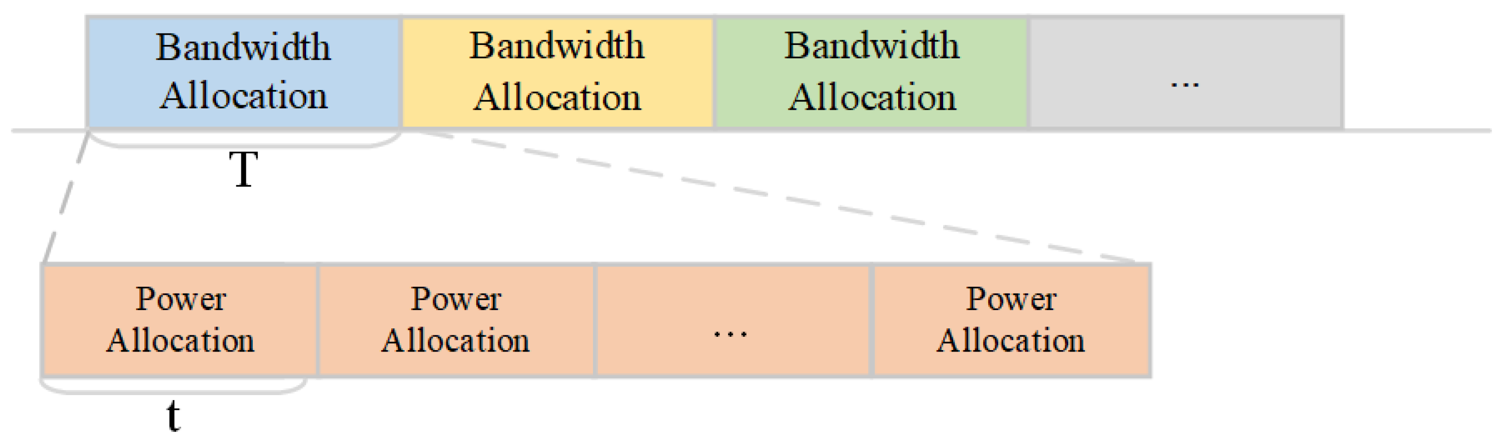
• A double-timescale framework is proposed in this paper to accommodate uneven time-varying traffic demands in aviation-type scenarios. In this framework, we allocate bandwidth and power on a large timescale, and subsequently allocate power on multiple small timescales. Compared to simultaneously adjusting the bandwidth and power resources, the double-timescale resource management approach enables us to fully and flexibly utilize all resources without compromising system stability, allowing for the better adaptation to the specific changes in aviation demands.
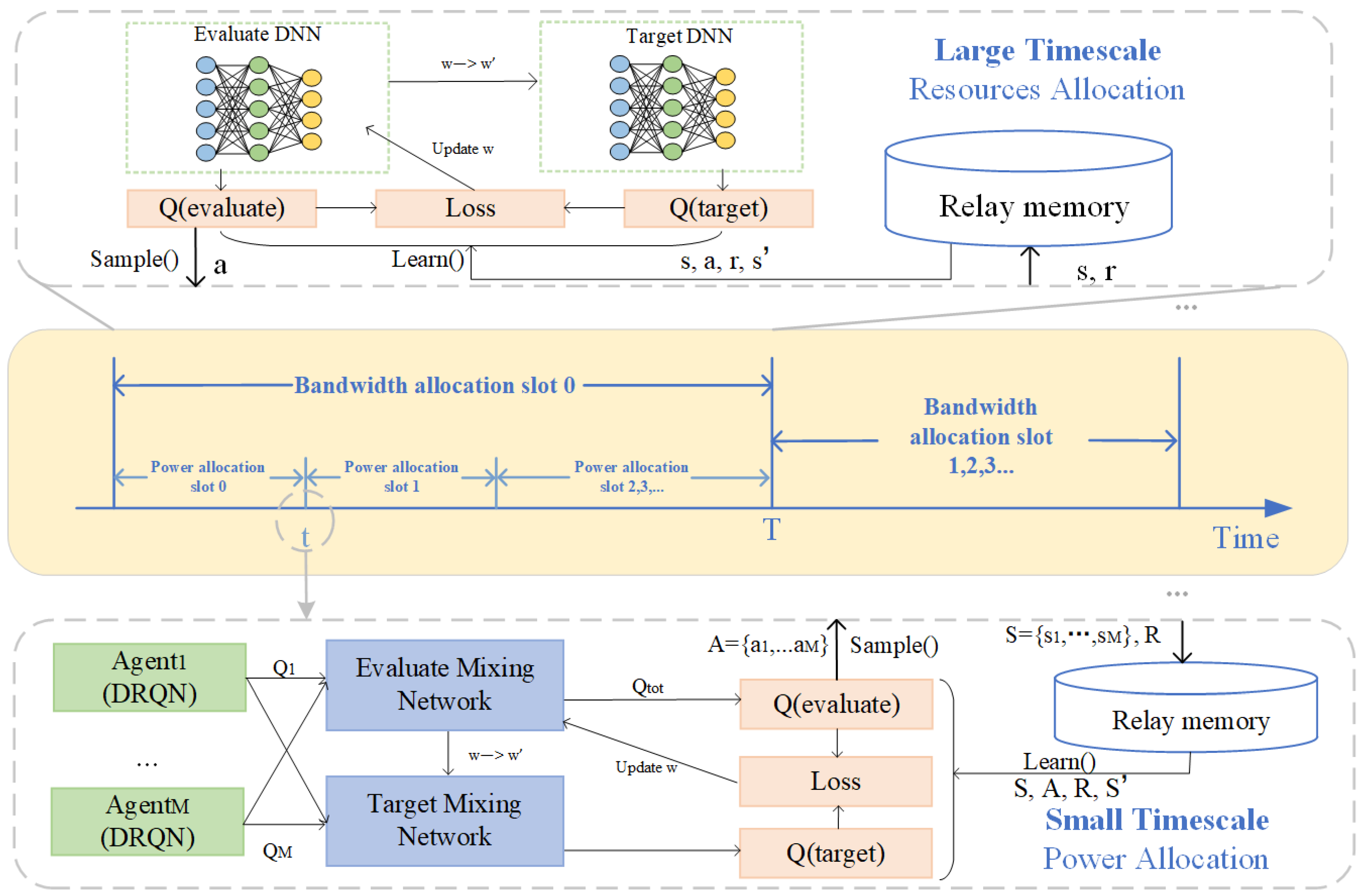
• The MADRL-based DT-BPA algorithm is employed to construct a two-layer network for addressing the DRM problem, which is low in complexity for offline training and online decision making. We model the DRM problem as a Markov decision process (MDP) and utilize DRL networks for offline training, which reduces the complexity of online execution to meet aviation demands in real time. Additionally, multi-agent method is used to cope with the exponential growth of the action space with the number of beams.
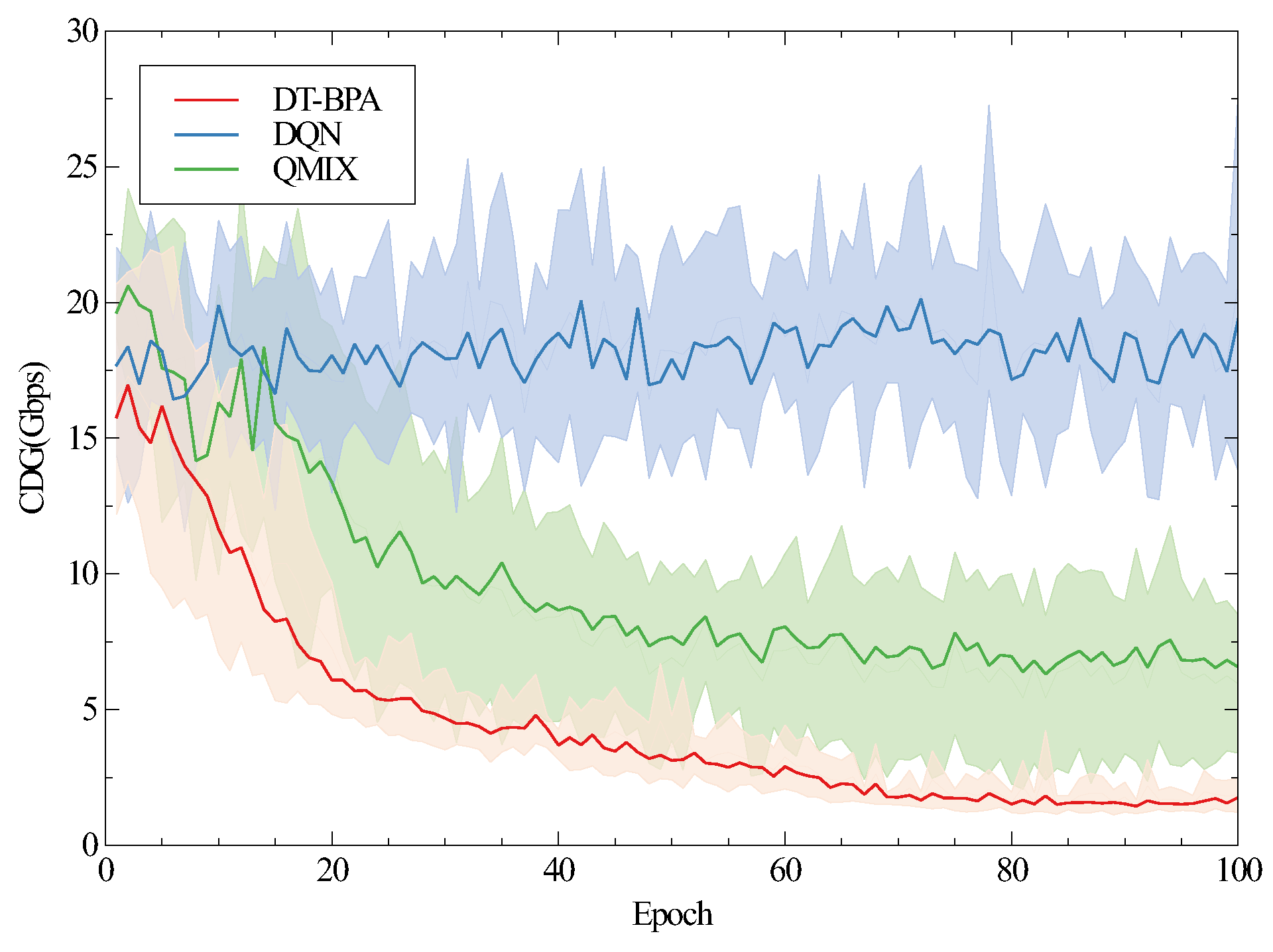
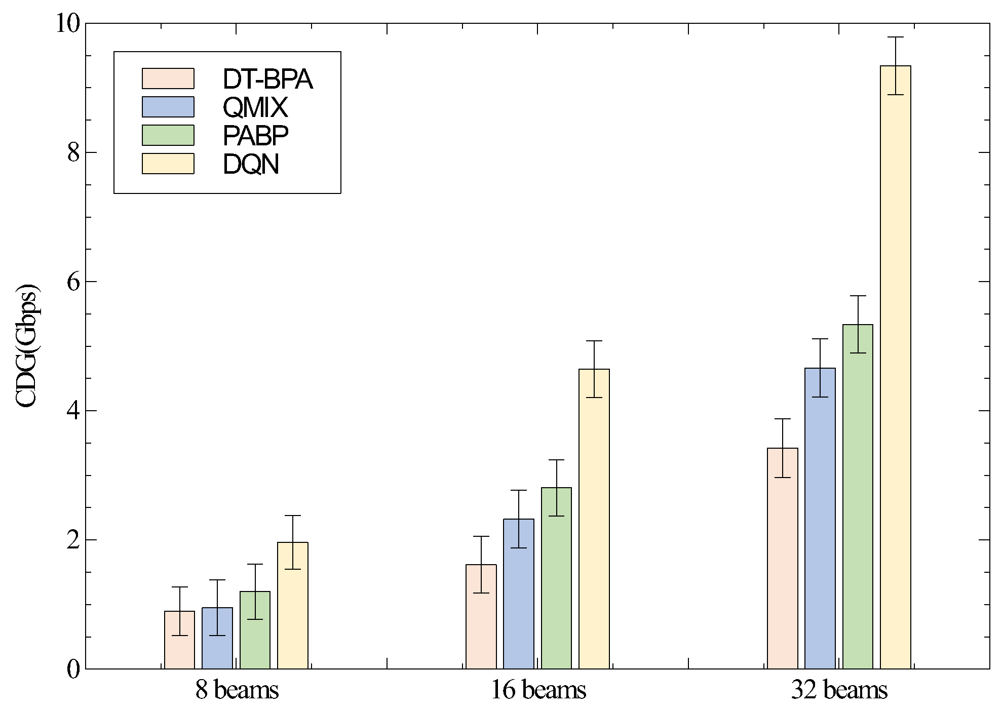
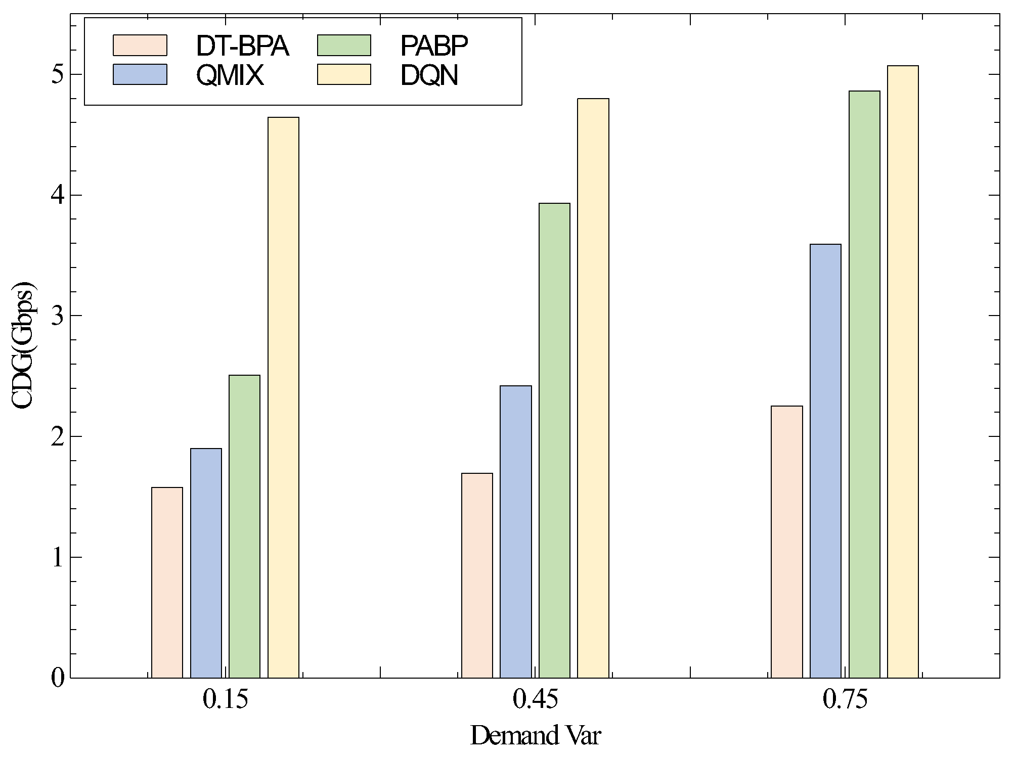
• We conduct extensive simulation experiments to evaluate the performance of the proposed scheme. The numerical results demonstrate that, when compared with the benchmark scheme, the proposed strategy can better match the multi-beam traffic demands over a long-time scale. The proposed scheme effectively utilizes the double-timescale resource management framework, enabling the better adaptation to time-varying traffic demands. On the premise of meeting the demand-matching degree, the power consumption of the system is also reduced, so the resource utilization and overall performance of the system are improved to a certain extent.

The rest of this paper is organized as follows. Section 2 summarizes the relevant work on the resource management of multi-beam satellite communication systems. Section 3 describes the VHTS model assumptions and architecture, and formulates issues about the dynamic management of power and bandwidth resource. Section 4 proposes the DT-BPA scheme using the MADRL algorithm and provides a detailed explanation of its implementation process. Section 5 presents simulation results and analysis. Section 6 provides a summary of the research.

2. Related Work

At present, research on resource allocation optimization in multi-beam satellite systems can be categorized into two directions: single-objective optimization and multi-objective optimization. To address the single-objective optimization problem of multi-beam satellite resource allocation, several optimization algorithms have been proposed, including traditional optimization algorithms [18,19], heuristic algorithms [20,21,22], and deep reinforcement learning algorithms [23,24]. For instance, Abdu et al. [19] decomposed the joint resource allocation problem into two sub-problems: carrier allocation and power allocation. Continuous carrier allocation (CCA) and interference-aware carrier allocation (IACA) are proposed, which are solved by the difference of the convex (DC) algorithm and successive convex approximation (SCA) algorithm, respectively. Paris et al. [22] used a genetic algorithm (GA) combined with repair functions to address the joint power and bandwidth resource allocation problem. Frequency re-use was considered to maximize the utilization of spectrum resources, and the unsatisfied system capacity (USC) was used as the objective function. However, the situation of the resource surplus was not considered. Cocco [21] and Paris et al. [22] observed that bandwidth flexibility had a more significant effect on improving the USC. Liao et al. [24] only studied the bandwidth allocation problem, and proposed a collaborative multi-agent deep reinforcement learning (CMDRL) framework to implement resource management strategies.

Due to the inclusion of various allocated resources such as bandwidth, power, carrier, beam size, beam position, etc., and the presence of multiple evaluation criteria and optimization objectives in the allocation algorithm, the DRM problem exhibits high complexity. For example, power consumption will lead to the reduction in the life of satellite components and bring challenges to the heat dissipation of satellites. Therefore, minimizing the total power consumption (TPC) of the system is also a key objective by optimizing the transmit power of each beam [25]. Therefore, the multi-objective optimization of the problem mainly adopts heuristic algorithm [26,27] and various learning algorithms [28,29]. For instance, Pachler et al. [27] studied the multi-objective optimization of the joint bandwidth and power allocation problem, using a combination of the USC and TPC objectives, and using an improved PSO-GA algorithm to solve the problem. The hybrid algorithm can reduce the TPC (up to 60%), and the increase in USC is less (only 2%). Ortiz-Gomez et al. [28] proposed the use of a machine learning (ML) algorithm to train bandwidth and power off-line in response to fluctuations of traffic demands. The optimization objectives encompassed minimizing the capacity demand gap (CDG), TPC, and total bandwidth consumption (TBC). However, the available bandwidth for each frequency reuse color was not constrained.

Table 1. Literature comparison of multi-beam satellite system resource allocation problem.

Type	Objective	Algorithm Classification	Concrete Algorithm	Demand Matching	Bandwidth Flexibility	Frequency Reuse	Power Flexibility	Literature
Single- objective	AFI	Convex optimization	Lagrange dual theory	×	×	×	✓	[18]
	USC, TPC, TBC	Convex optimization	DC, SCA	✓	✓	×	✓	[19]
	TPC	Heuristics	PSO	×	×	×	✓	[20]
	CDG, AFI	Heuristics	SA	✓	✓	×	✓	[21]
	USC	Heuristics	GA	✓	✓	✓	✓	[22]
	TPC	Deep reinforcement learning	DRL-DPA	×	×	×	✓	[23]
	CDG, AFI	Deep reinforcement learning	DRL-DBA	✓	✓	×	×	[24]
Multi- objective	USC, TPC	Heuristics	GA-SA, NSGA-II	✓	×	×	✓	[26]
	USC, TPC	Heuristics	PSO-GA, NSGA-II	✓	✓	×	✓	[27]
	CDG, TPC, TBC	Machine learning	SL	✓	✓	×	✓	[28]
	USC, TPC	Deep reinforcement learning	PPO	✓	×	×	✓	[29]

compares the resource allocation problems of multi-beam satellite systems in the literature from the aspects of optimization objectives, optimization algorithms, and whether to consider demand matching and resource flexibility.

In order to cope with the challenge that convex optimization algorithms and heuristic algorithms do not match the multi-beam real-time DRM problem, more and more studies have proposed the use of reinforcement learning technology to solve the problem of resource management in satellite communication. Hu et al. [30] demonstrated that the DRL framework is an effective method for wireless resource allocation. Bi et al. [31] discussed the advantages of the DRL framework using a model-free method in solving resource management problems. Liu et al. [32] also verified the strong performance of centralized DRL in real-time resource management. Ferreira et al. [33] used DRL technology in satellite communication to overcome the assumption limitations of other resource allocation methods. Ortiz-Gomez et al. [34] showed that the use of a multi-agent method can reduce the computational complexity and improve the scalability of the system.

By analyzing the resource allocation problem for multi-beam satellite systems, fewer studies have focused on adjusting the different types of resource allocation at different time scales to balance resource utilization and system stability. The VHTS system should be able to formulate an appropriate adjustment strategy according to the special business scenarios with the fixed routes. To this end, we propose the DT-BPA scheme and use the MADRL algorithm to deal with the DRM problem, where each agent only makes decisions on the power of one beam. Unlike previous studies, the VHTS system studied in this paper uses the frequency reuse scheme. Geographically isolated beams will use the same bandwidth, so a single agent decides the bandwidth of different reused bands.

3. System Model and Problem Formulation

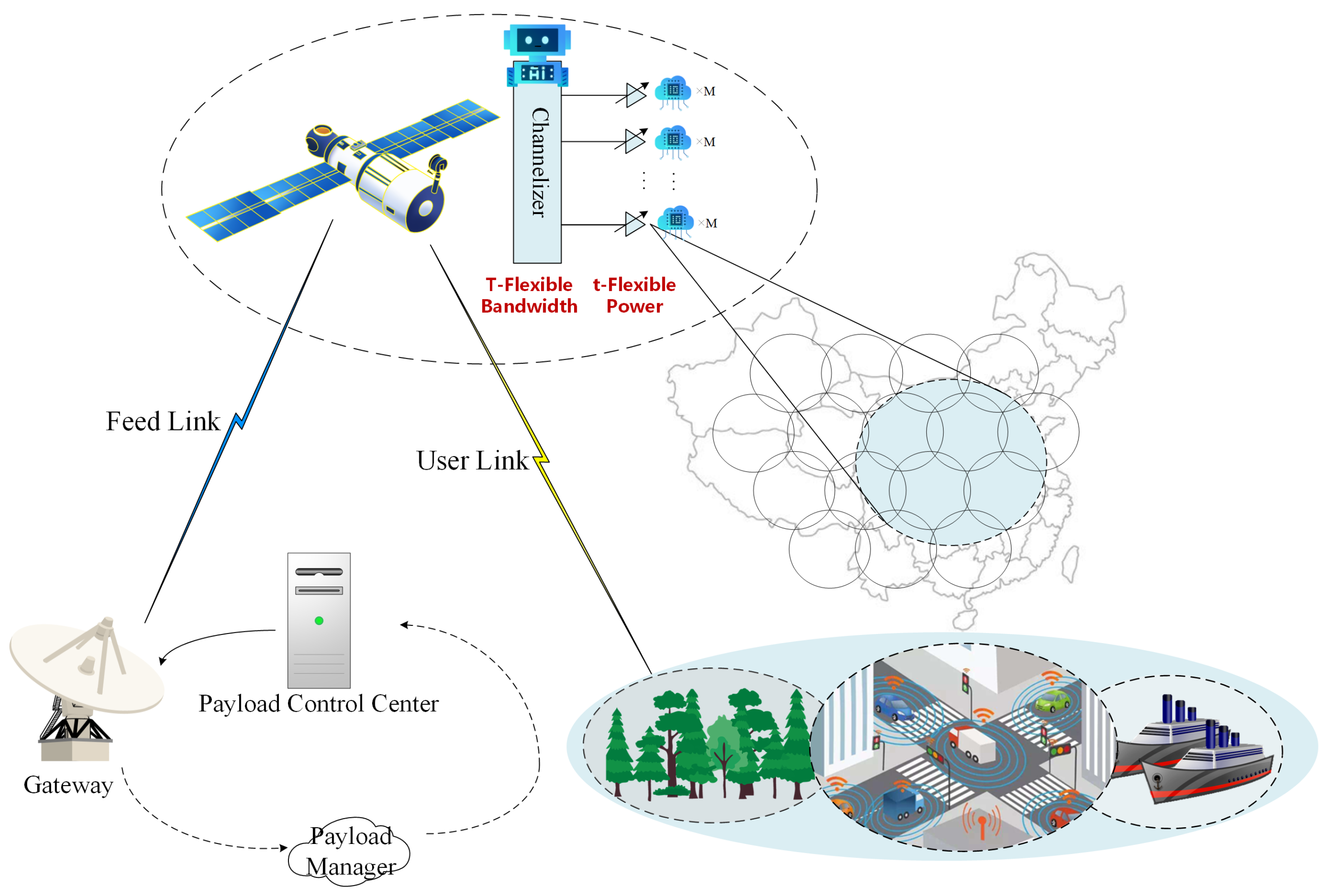
3.1. System Model

We propose a VHTS system model that utilizes a GEO satellite with multiple spot beams for communication and multiple gateway stations to accommodate the high bandwidth required by the feeder link. To confine the DRM problem to the beam level, we set the following assumptions for the VHTS system [35]. Firstly, we assume that the power or bandwidth between intra-beam carriers is allocated in a proportional fixed allocation mode. Secondly, we aggregate the traffic demands of all users within a beam to obtain the total demands of the beam, and the resource allocation among users in the beam is based on existing literature. Finally, the beams in the model are spot beams, assuming that beam hopping and timeslot allocation are not used.

The payload considered by the VHTS system should be able to flexibly manage two types of resources, namely power and bandwidth. Therefore, it is assumed that the satellite payload is equipped with the necessary modules, including flexible traveling wave tube amplifiers (TWTA) and channelizers. The TWTA dynamically allocates power to its associated beams based on the input power back-off, enabling flexible power management. The channelizer separates the signal into frequency blocks and rearranges them based on instructions to achieve flexible bandwidth allocation. The flexibility of these resources is realized through the architecture depicted in Figure 1. The payload manager receives input demand data, generates the optimal resource allocation result through the network control center, and transmits it to the satellite, thereby influencing the user links.

The VHTS system utilizes the limited spectrum more effectively through multi-color frequency reuse, enabling high-speed broadband data transmission. Figure 2a depicts a schematic 19-beam layout. Taking the simplest practical reuse pattern, the four-color reuse pattern (involving two frequencies and two polarizations) [36], as an example, the beams assigned with yellow and blue colors use left-handed circular polarization (LHCP), while the beams assigned with red and green colors use right-handed circular polarization (RHCP). When allocating bandwidth resources, beams with different polarizations are independent. Adjacent beams with the same polarization can exchange bandwidth, as shown in Figure 2b. We assume that adjacent beams cannot use overlapping frequency ranges, otherwise strong inter-beam interference will occur. The DRM scheme proposed below is suitable for any frequency reuse mode.

We assume that a very-high-throughput GEO satellite is configured with B beams. The total power of the VHTS system is denoted by $P_{tot}$, while the total bandwidth of the VHTS system is represented by $B{W}_{tot}$. The transmission power of the b-beam is $P_b$, and the bandwidth of the b-beam is $B{W}_b$. The system includes $N_a$ amplifiers, where $N_a\le B$, the maximum power allowed by amplifier a is $P_{max}^a$. Each beam is connected to one and only one amplifier, and each amplifier can be connected to multiple beams. The system adopts the TWTA to manage the power allocation adjustment. To meet the power constraints, the power allocated to the b-beam must not exceed the upper limit defined for each beam. The beam power cap constraint is expressed as

$$P_t^b\le P_{max}^b.$$

(1)

Additionally, the sum of the power allocated to all beams should not exceed the total power of the system. The total power constraint is expressed as

$$\sum _{b=1}^B{P}_t^b\le P_{tot}.$$

(2)

Moreover, the sum of the power allocated to beams connected to the same amplifier must not exceed the maximum power allowed by the amplifier. The amplifier power constraint is expressed as

$$\sum _{b=1}^B{P}_t^{b,a}\le P_{max}^a,$$

(3)

$$P_t^{b,a}=\left\{\begin{array}{cc}{P}_t^b,& bconnectedtoa\\ 0,& bnotconnectedtoa\end{array}\right..$$

(4)

The channelizer is used to manage the adjustment of bandwidth allocation in the system. The system adopts a dual-polarized multi-color frequency reuse pattern. Adjacent beams with the same polarization can exchange bandwidth when allocating bandwidth. As shown in Figure 2, the No. 1 beam and the No. 3 beam are adjacent in position and have the same polarization direction in the spectrum, so the two beams can exchange bandwidth. The sum of bandwidth allocated to different frequency colors of the same polarization in the bandwidth plan is equal to the total bandwidth of the system. The bandwidth constraint is expressed as

$$\sum _{j=1}^{J}B{W}_{i,j}=B{W}_{tot},i=0,1,$$

(5)

where i denotes the frequency polarization direction, $i=0$ denotes the left polarization, and $i=1$ denotes the right polarization. J denotes the number of sub-bands of the same polarization direction. ${BW}_{i,j}$ denotes the bandwidth of the sub-band j of the polarization direction i.

The VHTS communication system in this paper adopts a double-timescale management strategy of bandwidth and power to flexibly meet the real-time traffic demands while maintaining the resource utilization and system stability. The management strategy consists of a large-timescale bandwidth and power allocation stage and a small-timescale power allocation stage, as shown in Figure 3. In the large-timescale resources allocation stage, the system allocates bandwidth to each sub-band and allocates power to each beam based on the resource constraints and the traffic demands over a period of time. In the small-timescale power allocation stage, the system allocates the power to each beam connected to all amplifiers based on the bandwidth allocation result, power resource constraints, and real-time traffic demands. Furthermore, the system needs to set reasonable time intervals and a corresponding proportion of different time scales according to the specific situation. The strategy can improve the performance and user experience of the satellite communication system, and provide customized services for different beams and users.

3.2. Link Budget

It is assumed that the capacity provided by the b-beam $C_b$ depends on the bandwidth allocated to the beam ${BW}_b$ and the spectral efficiency of the beam ${SE}_b$, which is specifically denoted as

$$C_b={BW}_b\times {SE}_b,$$

(6)

where ${SE}_b$ is the spectral efficiency of the modulation and coding schemes used by commercial modems. Due to the variation in the beam gain and transmission channel conditions within the coverage range, each beam will experience different carrier-to-interference-plus-noise ratios. By referring to the DVB-S2X system, the relationship between the spectral efficiency of each beam and the carrier-to-interference-plus-noise ratio ${CINR}_{total}$ is modeled by a general function $f_1\left(·\right)$. The DRM problem is a discrete problem since $f_1\left(·\right)$ is a step function.

$${SE}_b=f_1\left(CIN{R}_{total}\right).$$

(7)

In the VHTS system, the feeder link from the gateway station to the satellite should be considered. The total carrier-to-interference-plus-noise ratio ${CINR}_{total}$ is related to the carrier-to-interference ratio ${CIR}_b$ and the carrier-to-noise ratio ${CNR}_b$.

The carrier-to-interference ratio $CI{R}_b$ represents the difference between the power allocated to the b-beam and the interference power of the b-beam, which is specifically denoted as

$$CI{R}_b=P_b-I_b.$$

(8)

The frequency color needs to be assigned to each beam before calculation. The principle is that the adjacent beams have different frequencies, and that the beams of the same frequency are as far apart as possible. The co-channel interference power $I_b$ is a function of the frequency reuse scheme and ${\theta }_b$, which is specifically denoted as

$$I_b=\sum _{\phi =1}^{\Phi }{P}_{co}\left(\varphi ,{\theta }_b\right),$$

(9)

where ${\theta }_b$ is the 3dB beamwidth of the b-beam, $\varphi$ represents the angle between the b-beam and the interference beam, $\Phi$ represents the total number of interference beams of the b-beam, and $P_{co}$ represents the interference power level of the $\phi$-th interference beam of the b-beam.

The calculation of the carrier-to-noise ratio $CN{R}_b$ is related to the b-beam power $P_b$, beam-transmitting antenna gain $G_b$, user-receiving antenna gain $G_u$, Boltzmann constant k, system temperature $T_s$, total link loss $L_b$, amplifier power back-off $OBO$, and the b-beam bandwidth ${BW}_b$. The specific expression of $CN{R}_b$ is

$$CN{R}_b=P_b+G_b+G_u/T_s-L_b-k-log\left(B{W}_b\right)-OBO.$$

(10)

The total link loss $L_b$ includes free space loss $L_{FS,b}$, atmospheric loss $L_{atm,b}$, transmission loss $L_{RF,b}$, and reception loss $L_{RF,u}$. The specific expression of $L_b$ is

$$L_b=L_{FS,b}+L_{atm,b}+L_{RF,b}+L_{RF,u}.$$

(11)

The relationship between transmitting antenna gain $G_b$ and beamwidth ${\theta }_b$ can be modeled by an appropriate function $f_2\left(·\right)$

$$G_b=f_2\left({\theta }_b\right).$$

(12)

3.3. Problem Formulation

The VHTS system manages both bandwidth and power resources through flexible payloads. The goal is to match the capacity provided by the beam with the traffic demand as much as possible. Therefore, we formulate CDG as the evaluation index of resource allocation results. The smaller the CDG, the higher the matching degree of capacity and demand.

$$CDG=\sum _{b=1}^B\left|D_t^b-C_t^b\right|.$$

(13)

The DRM objective function is defined as minimizing the average CDG per time to achieve the optimal matching of capacity and demand within T time. In addition, to ensure the reliable operation of the equipment and prolong its service life, the TPC is minimized under the premise of ensuring capacity and demand matching. Based on the above analysis, the DRM problem is defined as

$$\underset{P_t^b,B{W}_b}{min}{F}_1=\frac{1}{T}\sum _{t=1}^T({\beta }_1\sum _{b=1}^B\left|D_t^b-C_t^b\right|+{\beta }_2\sum _{b=1}^B{P}_t^b)$$

(14)

$$s.t.P_t^b\le P_{max}^b,b=1,2,\dots ,B,$$

(15)

$$\sum _{b=1}^B{P}_t^{b,a}\le P_{max}^a,a=1,2,\dots ,N_a,$$

(16)

$$\sum _{b=1}^B{P}_t^b\le P_{tot},$$

(17)

$$B{W}_b\le B{W}_{tot},$$

(18)

$$\sum _{j=1}^{J}B{W}_{i,j}=B{W}_{tot},i=0,1.$$

(19)

The DRM objective function $F_1$ minimizes two parameters of the average time, representing the performance index and the cost index, respectively. The performance index is designed to measure the degree to which the system capacity meets the demand, and it is represented by the CDG. The weight of CDG in the objective function is denoted by ${\beta }_1$. On the other hand, the cost index is designed to measure the resource consumption that meets all beam demands. Assuming that VHTS uses all bandwidth resources, the selected index is the power of all beams in the satellite, where ${\beta }_2$ is the weight of TPC. Among them, (15)–(17) are power constraints, and (18) and (19) are bandwidth constraints. The formulated optimization problem is a nonlinear and discrete function with multiple constraints. Considering the complexity characteristics of the formulated problem, the double-timescale MADRL method is adopted to solve the formulated DRM problem.

4. Double-Timescale MADRL Algorithm

The VHTS system is characterized by a large number of beams, rapid demand changes, and significant differences in the demand between beams. Consequently, the computational complexity of the double-timescale DRM problem is extremely high. To address this issue, we reconstruct the DRM problem into a DT-MADRL problem. The key idea behind the DT-MADRL approach is to employ a single agent to manage the bandwidth of each sub-band in multi-color reuse using the Deep Q-Network (DQN) for training. Additionally, B agents are utilized to manage the power of all beams connected by different amplifiers in the satellite system, with the traffic demands of beams acting as the environment. The B agents share the same resource allocation space and are trained using the QMIX network. When different traffic demand data are input, the network can output the bandwidth and power allocation results that meet the optimization objectives. We assume that the amplifier can connect any number of beams, and the power management network corresponding to each amplifier is independent. Consequently, we can train the power management network first. For the trained network, it is required that, for all possible traffic demands and bandwidth inputs, the power values that achieve the optimal matching of beam capacity and demand in the amplifier can be obtained. The trained power management network parameters of each amplifier are imported as the environment to train the whole system resource management network. For the trained network, it is required to be able to obtain the bandwidth and power that achieve the optimal matching of beam capacity and demand in the system according to all possible traffic demands inputs. The DT-BPA scheme using the MADRL algorithm architecture is shown in Figure 4. Both models use the evaluation network and the target network, as well as experience a replay buffer, which ensure the stability of the learning.

4.1. Small-Timescale Power Allocation Strategy

For the power management network at a small time scale, the power allocation of the beams connected to each amplifier is required. The objective is to achieve the optimal matching of the beam capacity and demand in the amplifier. On this basis, the TPC of beams in the amplifier is minimized to reduce the device power consumption and extended service life. The offline-trained power management network can adapt to traffic variations in real-time and automatically adjust strategies. The multi-agent method adopted by the network can readily accommodate scenarios with an increasing number of beams by simply adding more agents. These features enable it to better integrate with resource management networks operating on a large time scale.

Based on the above objectives, we assume that the amplifier is connected to M beams and model M agents to manage the power allocation of beams connected to the amplifier. All agents operate in a fully cooperative manner. It is believed that the maximum reward for the system requires the coordination of all agents, that is, the ultimate goal of all agents is to minimize the weighted sum of CDG and TPC of the beams in the amplifier. Since a single agent cannot obtain complete state information, the multi-beam cooperative power allocation decision process is modeled as a decentralized partially observable Markov decision process (Dec-POMDP), which is defined by tuples $<\mathcal{M},S,O,A,P,R,\gamma >$, where $\mathcal{M}=\{1,2,\dots ,M\}$ represents the set of agents. S denotes the set of environmental states, and O denotes the set of joint observations. A denotes the set of joint action space, and each agent $m\in M$ selects an action $a^m\in A^m$ to form a joint action $a\in A$. The joint action is applied to the environment, and then the next state is obtained. The corresponding transfer equation is $P(s\prime |s,a):S\times A\times S\to \left[0,1\right]$. $R\left(s,a\right):S\times A\to R$ denotes the reward function. $\gamma \in \left[0,1\right]$ represents a discount factor.

• State space

The environment of each time slot t includes the following. $D_t=\{D_t^1,D_t^2,\dots ,D_t^M\}$ represents the traffic demands of beams connected to the same amplifier, $C_t=\{C_t^1,C_t^2,\dots ,C_t^M\}$ represents the capacity provided by the beams, ${\Delta }_t=\{{\Delta }_t^1,{\Delta }_t^2,\dots ,{\Delta }_t^M\}$ represents the CDG of beams, $P_t=\{P_t^1,P_t^2,\dots ,P_t^M\}$ represents the current power allocated to beams, and $B{W}_t=\{B{W}_t^1,B{W}_t^2,\dots ,B{W}_t^M\}$ represents the current bandwidth allocated to the beams. Therefore, $S_t=\{O_t^1,O_t^2,\dots ,O_t^M\}$ represents the current state of M agents, where $O_t^m$ indicates the bandwidth, power, traffic demand, and CDG of the current beam m.

$$O_t^m=\{B{W}_t^m,P_t^m,D_t^m,{\Delta }_t^m\}.$$

(20)

2.

Action space

The action space represents the adjustment strategy of the agents for power allocation, and determines the power change of each beam. Specifically, $A_t=\{a_t^1,a_t^2,\dots ,a_t^M\}$ represents the action of M agents, that is, their movement in the space of possible allocated power resources, where $a_t^m$ refers to the possible action space of agent m, and represents the power increase or decrease or unchanged in m-beam.

$$a_t^m=\left\{\begin{array}{cc}{a}_1,& increaseinpower\\ a_2,& decreaseinpower\\ a_3,& donothing\end{array}\right..$$

(21)

3.

Reward

M agents share the same instant reward

$$r_t=-{\alpha }_1{F}_t+{\alpha }_2{F}_{t-1}-{\alpha }_3{P}_{pun},$$

(22)

$$F=f_3({\sum }_{b=1}^M({\beta }_1{\Delta }_b^2+{\beta }_2{P}_b)),$$

(23)

$$P_{pun}=\left\{\begin{array}{c}K,{\displaystyle \sum _{b=1}^M}{P}_b>P_{max}^a\\ 0,{\displaystyle \sum _{b=1}^M}{P}_b\le P_{max}^a\end{array}\right.,$$

(24)

where F denotes the measurement of the weighted sum of the CDG and the TPC of the beams in the amplifier. $P_{pun}$ represents the penalty term of amplifier power limit. In addition, ${\alpha }_1,{\alpha }_2,{\alpha }_3$ are positive values, indicating the weight of each parameter in the instant reward.

4.

Value function

The action-observation history of each agent is expressed as ${\tau }^m\in T\equiv {(O\times A^m)}^{\ast }$, that is, the sequential action-observation history starting from the initial state. The corresponding sequential action-observation history of all agents can be expressed as $\tau =({\tau }^1,{\tau }^2,\dots ,{\tau }^M)$. Based on this, the random strategy function of each agent is expressed as ${\pi }^m\left(a^m\right|{\tau }^m):T\times A\to [0,1]$. The joint action value function corresponding to the joint strategy is expressed as

$$Q_{tot}^{\pi }(\tau ,a)=E_{\tau \in T^M,a\in A}[\sum _{t=0}^{\infty }{\gamma }^{t}r(s,a)].$$

(25)

At this time, the value function is related to the action-observation history, not to the state.

The power management network is trained by the QMIX network, which consists of a mixing network and M agent networks. By using the centralized training-distributed execution (CTDE) method, the local action–value functions are learned in a distributed manner, and then the joint action-value function is constructed by concentrating all the local action-value functions. The joint reward of all agents is assigned to each agent, promoting cooperation among multiple agents to achieve maximum global benefits.

When dealing with the problem of multi-agent collaboration, two aspects need to be considered. One is how to learn the joint action–value function, and the other is how to decompose a reasonably distributed strategy from the joint value function. For centralized learning, the mixing network estimates the joint Q-value as a complex nonlinear combination of each agent’s Q-value. The network imposes constraints on the structure, so that the joint Q-value function is monotonic with each agent’s Q-value function, ensuring consistency between the centralized strategy and the decentralized strategy. Specifically, the specific individual-global-max (IGM) constraints are as follows:

$$\underset{a}{argmax}{Q}_{tot}(\tau ,a)=\left(\begin{array}{c}argma{x}_{a^1}{Q}_1({\tau }^1,a^1)\\ \dots \\ argma{x}_{a^m}{Q}_m({\tau }^m,a^m)\\ \dots \\ argma{x}_{a^M}{Q}_M({\tau }^M,a^M)\end{array}\right),$$

(26)

where $Q_{tot}$ represents the joint Q-value function, and $Q_m$ represents the Q-value function of the agent m. In order to guarantee the above conditions, the QMIX network is restricted by monotonic conditions.

$$\frac{\partial Q_{tot}}{\partial Q_m}\ge 0,\forall m\in \{1,2,\dots ,M\}.$$

(27)

For the distribution strategy, after obtaining the estimation of the global Q-value function, QMIX selects the action based on the local Q-value function and the output of the hybrid network, combined with the $\epsilon$-greedy algorithm. By adjusting $\epsilon$, the trade-off between exploration and exploitation can be controlled. A higher value of $\epsilon$ encourages the agent to explore and choose random actions to discover new strategies, while a lower value of $\epsilon$ encourages the agent to exploit and select the action with the highest Q-value to utilize the learned strategy. The update method of the mixing network is similar to that of DQN, as both use temporal difference-error for network self-renewal. In addition, the evaluation network and target network are both set up. The QMIX network loss function is

$$L\left(\omega \right)=\sum _{i=1}^b\left[{(y_i^{tot}-Q_{tot}(\tau ,a,s;\omega ))}^2\right],$$

(28)

where b represents the number of samples sampled from the experience relay buffer. $y^{tot}$ is expressed as

$$y^{tot}=r+\gamma {max}_{a^{\prime }}{Q}_{tot}({\tau }^{\prime },a^{\prime },s^{\prime };{\omega }^{-}),$$

(29)

where ${\omega }^{-}$ is a parameter of the target network, so the temporal difference-error can be expressed as

$$\delta =r+\gamma Q_{tot}\left(target\right)-Q_{tot}\left(evaluate\right),$$

(30)

where $Q_{tot}\left(target\right)$ represents the maximum value $Q_{tot}$ that can be obtained in all behaviors in the case of next state, and $Q_{tot}\left(evaluate\right)$ represents the $Q_{tot}$ obtained according to the behavior selected by the current network strategy in the case of current state.

Since MADRL is trained offline, the training process can be cut off once the network performance has finally converged. Therefore, only the complexity of the proposed algorithm in the online execution phase needs to be analyzed. The computational complexity of the execution refers to the complexity of computing the Q-value, which is related to the network structure. Since each agent chooses the action in parallel, the computational complexity of the proposed algorithm is determined by the most complex neural network of all agents. Assuming that $L_{\mathrm{QMIX}}$ and $n_{\mathrm{i}}^{\mathrm{QMIX}}$ denote the number of layers of the deep neural networks (DNNs) and the number of neurons in layer i used by the DT-BPA algorithm for the small time scale power allocation network, respectively, the execution computational complexity is $O({\displaystyle \sum _{i=1}^{L_{QMIX}-1}}{n}_i^{QMIX}{n}_{i+1}^{QMIX})$ [37]. The specific algorithm process is shown in Algorithm 1.

Algorithm 1 QMIX-based power allocation algorithm.

Input: network parameters and system parameters. Output: power allocation strategy.   1: for $epoch=1,2,\dots ,N_{epoch}$ do   2:    for $episode=1,2,\dots ,N_{episode}$ do   3:      Initialize environment, obtain the state S, the observation of each agent $O^m$, the available action of each agent $A^m$, and reward R.   4:      for $t=1,2,\dots ,N_{step}$ do   5:         Each agent uses eval_agent_network obtains the Q-value of each action. With probability $\epsilon$ select a random action $a_t^b$, otherwise select the action that maximizes the Q-value.   6:         Store $S,S_{next}$, the observation values of each agent $O^m$, the available action of each agent $A^m$, the next action of each agent $A_{next}^m$, the reward R, the selected action a, whether env has terminated $terminate$, in the experience pool D.   7:         Randomly sample some data from D, but the data must be the same transition in different episodes.   8:         Update Parameters:         $L\left(\omega \right)={\sum }_{i=1}^b[(y_i^{tot}-Q_{tot}(\tau ,a,s;\omega ){)}^2]$   9:         if $terminate==Trueandstep\le N_{step}$ then 10:           for $k=stepto{N}_{step}$ do 11:              Fill in the insufficient data with 0 to ensure data consistency. 12:           end for 13:         end if 14:         $S=S_{next},A^m=A_{next}^m$ 15:         if $t\%p(\mathrm{update}\mathrm{frequency})==0$ then 16:           Copy the evaluation network parameters to the target network. 17:         end if 18:      end for 19:    end for 20:    Calculate the average reward of $N_{episode}$ episodes and add it to the list. 21: end for

4.2. Large-Timescale Resources Allocation Strategy

The resources management network on a large time-scale requires the allocation of bandwidth for different color sub-bands and power for different beams in the VHTS system. After obtaining the sub-band bandwidth and initial beam power on a large time-scale based on the average traffic demands over a period of time, the trained power management network is employed to allocate power at subsequent time points during that period. The objective is to achieve an optimal matching of beam capacity and demand in the system. Based on the stated objectives, we assume that the VHTS system consists of B beams. We model a single agent to manage the bandwidth allocation of M frequency colors and B agents to handle power allocation for all beams. Additionally, we import the parameters of the converged power management network model as environment variables, eliminating the need to retrain the power allocation process. The shared goal of all agents is to minimize the weighted sum of the CDG and TPC of the beams in the system. Assuming that the agent managing the bandwidth has access to complete state information, the bandwidth allocation decision process is modeled as MDP defined by tuples $<S,A,P,r,\gamma >$. The strategy gives the corresponding feasible action $A_t$ according to the given state $S_t$ and action–value function, and then, the agent obtains the reward $r_t$ for taking action. The state of the system is converted into $S_{t+1}$, where the state transition probability is $P(s_{t+1},r_t|s_t,a_t)$, and the corresponding strategy is $\pi \left(a_t\right|s_t)$, $\gamma \in \left[0,1\right]$ represents the discount factor.

• State space

The environment of each time slot t includes the following. $D_t=\{D_t^1,D_t^2,\dots ,D_t^{\mathrm{B}}\}$ represents the traffic demand of B beams, $C_t=\{C_t^1,C_t^2,\dots ,C_t^{\mathrm{B}}\}$ represents the capacity provided by B beams, ${\Delta }_t=\{{\Delta }_t^1,{\Delta }_t^2,\dots ,{\Delta }_t^B\}$ represents the CDG of B beams, $P_t=\{P_t^1,P_t^2,\dots ,P_t^{\mathrm{B}}\}$ represents the current power of B beams, $B{W}_t=\{B{W}_t^1,B{W}_t^2,\dots ,B{W}_t^M\}$ represents the current bandwidth of M frequency colors, and ${\omega }_t$ represents the parameters of the power management network. Therefore, $S_t$ represents the current state of the agent managing the bandwidth allocation, indicating the current bandwidth, power, traffic demand, and CDG of all beams in the system.

$$S_t=\{B{W}_t,P_t,D_t,{\Delta }_t\}.$$

(31)

2.

Action space

The action space represents the adjustment strategy of the agent for bandwidth allocation, and determines the bandwidth change of each frequency color. $A_t$ represents the action of the bandwidth agent, that is, its movement in the space of bandwidth resources that may be allocated. There are $3^M$ possible actions, indicating that the bandwidth of M frequency colors is increased or decreased or unchanged.

3.

Reward

The instant reward of the bandwidth agent is

$$r_t=-{\alpha }_1{H}_t+{\alpha }_2{H}_{t-1},$$

(32)

$$H=f_4({\sum }_{b=1}^B({\beta }_1{\Delta }_b^2+{\beta }_2{P}_b)),$$

(33)

where H is the measure of the weighted sum of the CDG and TPC of all beams in the system. Similarly, ${\alpha }_1,{\alpha }_2$ are positive values, indicating the weight of each parameter in the instant reward.

The DQN generation function is used to estimate the action value. Based on the current Q-value estimation, the strategy is used to select an action, which is then executed by the bandwidth agent. The other B power agents perform multi-step adjustments according to the trained network to obtain the optimal power allocation at that time. The agents observe the immediate reward r returned by the environment and the next state $s^{\prime }$. We add the current state, action, reward, and next state to the experience relay buffer. Subsequently, a batch of experience samples is randomly sampled from the experience replay buffer to train the neural network. The target Q-value of the sample is

$$Q_{target}=r+\gamma maxQ\left(s^{\prime },a^{\prime };{\theta }^{-}\right),$$

(34)

where r is the instant reward, $s^{\prime }$ is the next state, $a^{\prime }$ is the optimal action of the next state, and $\gamma$ is the discount factor, ${\theta }^{-}$ is the parameter of the target network.

The mean square error (MSE) loss function is employed to quantify the disparity between the current Q-value estimation and the target Q-value. By utilizing backpropagation, the parameters of the neural network are adjusted to minimize this loss

$$L\left(\theta \right)=\frac{1}{2}{[Q_{target}-Q(s,a;\theta )]}^2.$$

(35)

The parameters of the target network are updated regularly by copying the current evaluation Q network parameters to the target network to enhance stability and convergence.

Assuming that $L_{\mathrm{DQN}}$ and $n_{\mathrm{i}}^{\mathrm{DQN}}$ denote the number of layers of the DNNs and the number of neurons in layer i used by the DT-BPA algorithm for the small time scale power allocation network, respectively, the execution computational complexity is $O({\displaystyle \sum _{i=1}^{L_{DQN}-1}}{n}_i^{DQN}{n}_{i+1}^{DQN})$. The specific algorithm process is shown in Algorithm 2.

Algorithm 2 DQN-based resources allocation algorithm.

Input: network parameters and system parameters. Output: bandwidth and power allocation strategy.   1: for $epoch=1,2,\dots ,N_{epoch}$ do   2:    for $episode=1,2,\dots ,N_{episode}$ do   3:      Initialize environment, obtain the state S, and reward R.   4:      for $t=1,2,\dots ,N_{step}$ do   5:         Each agent uses eval_network obtains the Q-value of each action. With probability $\epsilon$ select a random action $a_t$, otherwise, select the action that maximizes the Q-value.   6:         Store $S,S_{next}$, the selected action of each agent a, whether env has terminated $terminate$, in the experience pool D.   7:         Randomly sample some data from D, but the data must be the same transition in different episodes.   8:         Update Parameters:         $L\left(\theta \right)={\sum }_{i=1}^b[(y_i-Q_{target}{)}^2]$   9:         if $terminate==Trueandstep\le N_{step}$ then 10:           for $k=stepto{N}_{step}$ do 11:              Fill in the insufficient data with 0 to ensure data consistency. 12:           end for 13:         end if 14:         $S=S_{next}$ 15:         if $t\%p(\mathrm{update}\mathrm{frequency})==0$ then 16:           Copy the evaluation network parameters to the target Network. 17:         end if 18:      end for 19:    end for 20:    Calculate the average reward of $N_{episode}$ episodes and add it to the list. 21: end for

5. Performance Evaluation

In this section, we employ Python simulations to show the performance of the proposed DT-BPA scheme in the VHTS system. We begin by presenting the simulation parameters. Subsequently, the convergence performance of the proposed algorithm is explained. Furthermore, we conduct simulations to analyze the performance of bandwidth and power resource management under various traffic demands. Finally, we compare the results with other algorithms to demonstrate the enhanced matching performance of the capacity and demand achieved by the proposed algorithm.

5.1. Simulation Setting

In the simulation scenario, we consider a very high-throughput GEO satellite that utilizes the Ka-band for communication. The channel gain primarily takes into account the free space propagation loss. The transmitting antenna gain depends on the antenna radiation pattern with a beamwidth of 0.6 degrees. The multi-beam antenna radiation pattern refers to the Rec. ITU-R S.672 [30]

$$G\left(\theta \right)=\left\{\begin{array}{c}{G}_m,for\theta <{\theta }_b\\ G_m-3{\left(\frac{\theta }{{\theta }_b}\right)}^2,for{\theta }_b\le \theta <a{\theta }_b\\ G_m+L_s,for\mathrm{a}{\theta }_b\le \theta <b{\theta }_b\\ max\{G_m+L_s+20-25lg\left(\frac{\theta }{{\theta }_b}\right),0\},else\end{array}\right..$$

(36)

The $G/T$ value of the receiving antenna at the client is 22 dB/K. It is assumed that the satellite consists of 16 spot beams and 4 TWTAs and adopts a dual-polarized four-color reuse pattern. The beams of different frequencies are connected to the same amplifier. The relationship between the SE of each beam and the carrier-to-interference-plus-noise ratio is determined as follows [38]. The SE value is selected from low to high, and the energy per bit to noise power spectral density ratio of the beam is calculated as

$$E_b/N_0=CIN{R}_{total}-10log\left(SE\right).$$

(37)

If this value is not less than the threshold corresponding to the SE, the beam can select the SE value until the highest SE value for the beam is reached. The correspondence between SE and the threshold is presented in

Table 2. Corresponding results of the SE-threshold.

SE	Threshold	SE	Threshold
0.83	1.8	2.22	5.6
1	2.2	2.5	6.3
1.11	2.6	2.67	6.8
1.25	3	2.78	7.2
1.33	3.4	3.13	7.8
1.39	3.8	3.33	8.5
1.5	3.9	3.47	8.9
1.67	4.6	3.7	10.1
1.88	5.4	3.75	10.4

. The specific system simulation parameters are outlined in

Table 3. Satellite system simulation parameters.

Parameters	Values
Satellite altitude h	35,786 km
Beam number B	16
System total power $P_{tot}$	1600 W
Amplifier maximum power $P_{max}^a$	400 W
System total bandwidth $B{W}_{tot}$	2 GHz
Beamwidth $\theta$	0.6°
Link loss $FSPL$	210 dB
Amplifier backlash $OBO$	3 dB
UT receiving $G_u/T_s$	22 dB/K
Boltzmann constant k	−228.6 dB
Amplifier number $N_a$	4
Frequency color number M	4
Frequency polar number $N_p$	2

. We input an episode to the network for training each time, and the algorithm simulation parameters are provided in

Table 4. Algorithm simulation parameters.

Parameters	Values
Step number $N_{step}$ (Qmix)	100
Epoch number $N_{epoch}$ (Qmix)	100
Episode number $N_{episode}$ (Qmix)	10
Step number $N_{step}$ (DQN)	50
Epoch number $N_{epoch}$ (DQN)	50
Episode number $N_{episode}$ (DQN)	12
Update frequency	100
Learning rate	0.001
Discount factor $\gamma$	0.98
Batch size	32

.

We compare the proposed DT-BPA algorithm with the four following algorithms.

• Single-timescale management of bandwidth and power: For the change in the traffic demands during a period, only the bandwidth and power resources are managed at the same time on a large timescale.
• Proportional allocation of bandwidth and power (PABP): For the difference in traffic demand of each beam, the power and bandwidth resources are allocated according to the proportion of demand.
• QMIX [39]: Each agent manages the bandwidth of each frequency color and the power of all beams using the bandwidth, and uses the QMIX algorithm for training.
• DQN [40]: Single agent manages the bandwidth of all frequency colors and the power of all beams in the system, and uses the DQN algorithm for training.

In this paper, CDG is taken as the performance index, which is defined as the sum of gaps between the beam capacity and the beam demand of the system. The distribution of traffic demand is related to the population density, geographical location and temporal variations during the day.

5.2. Simulation Results

Figure 5 and Figure 6 illustrate the convergence trends of the reward and CDG of the three DRL algorithms during the training process. It can be seen that the DT-BPA algorithm and the QMIX algorithm start to converge at approximately 70 epochs, while the DQN algorithm does not converge in the end. Initially, the action is performed randomly, resulting in a smaller reward. However, as agents continue to learn and improve their actions, rewards gradually increase. The DT-BPA algorithm has a higher final convergence reward value and a smaller CDG than the QMIX algorithm, which indicates that the DT-BPA algorithm is better. The phenomenon lies in the QMIX algorithm where a single agent manages too many resources, resulting in an overly large action space. Consequently, it becomes difficult to effectively schedule resources in tandem with changing demands, usually leading to suboptimal outcomes confined within local optima.

Figure 7 illustrates the CDG obtained by different resource management algorithms as the number of beams in the VHTS system changes. Input multiple sets of traffic demands with different distributions, and calculate the average and standard deviation of the obtained CDG. By comparing the proposed DT-BPA algorithm with the PABP, QMIX and DQN algorithms, it is evident that the DT-BPA algorithm achieves the smallest CDG across different numbers of beams. It indicates that the DT-BPA algorithm optimally matches the system’s capacity with the demand, ensuring an optimal utilization of resources. Since the DQN did not converge, it was equivalent to random allocation, resulting in the worst performance. When the number of system beams is relatively small, the proposed algorithm is not much different from QMIX and PBAP. However, as the number of beams increases, the superiority of the proposed DT-BPA algorithm becomes more prominent, indicating that our algorithm is suitable for the current VHTS system with a large number of beams.

Figure 8 presents the TPC obtained by different resource management algorithms as the number of beams in the VHTS system changes. Input multiple sets of traffic demands with different distributions, and calculate the average and standard deviation of the obtained TPC. The PABP algorithm allocates all resources according to the proportion of the demands of different beams, so the TPC is fixed. By comparing the DT-BPA algorithm with the PABP, QMIX, and DQN algorithms, it can be seen that the DT-BPA algorithm consistently achieves the lowest TPC across the different numbers of beams. This indicates that the DT-BPA algorithm effectively minimizes the power consumption of the system, contributing to increased service life.

Figure 9 shows the CDG obtained by different resource management algorithms with 16 beams as an example in the case of traffic demands with different variances. When the total demand of the system is fixed, the higher the variance of traffic demand data of each beam, the more heterogeneous the distribution of the demands becomes. By comparing the proposed DT-BPA algorithm with PABP, QMIX, and DQN algorithms, it is evident that the DT-BPA algorithm achieves the minimum CDG under varying demand distributions, exhibiting the least susceptibility to the influence of uneven demand distribution, with the QMIX algorithm ranking second. The PABP algorithm allocates the resources according to the proportion of each beam demand, so it is most affected by the uneven distribution of demands. Due to its inability to converge, the DQN algorithm resorts to random allocation regardless of the demand distribution, resulting in a largely unchanged CDG.

Figure 10 compares the system capacity results of double-timescale and single-timescale resource management within a day. In the case of double-timescale resource management, we adjust the bandwidth and power based on the average demand for the next six hours at 0:00, 6:00, 12:00, and 18:00. Additionally, we adjust the power every hour according to the current demand. In the case of single-timescale resource management, the bandwidth and power resources are adjusted simultaneously based on the average demand only four times to satisfy the traffic demand for the whole day as much as possible. It is evident that, despite significant fluctuations in traffic demand over time, the double-timescale resource management algorithm still achieves the satisfactory matching of capacity and demand. It demonstrates the effectiveness of managing both bandwidth and power resources on different timescales.

Figure 11 depicts the demands and capacities of 16 beams in the system based on the DT-BPA algorithm as the total demand keeps increasing. We can note that the proposed algorithm almost matches the capacities provided by all beams with the demands for a total demand of 21 Gbps at the 0:00 and 40 Gbps at the 19:00. The capacities and demands of individual beams show a relatively large gap, which can be attributed to the frequency reuse scheme of the system. As a result of this scheme, some beams share the same bandwidth resources and are weighted according to the traffic demands associated with each beam. However, when the total system demand surges to 60 Gbps, which exceeds the capacity that can be provided by the system resources, the demand of each beam is difficult to meet. In this case, the system requires additional system optimization or capacity expansion measures.

6. Conclusions

In this paper, we proposed a DT-BPA scheme to address the bandwidth and power resource management problem in VHTS systems. Our objective was to achieve efficient resource allocation while ensuring that the capacity provided by each beam closely matches the traffic demand over a given time period, considering the frequency reuse scheme. To tackle this problem, we employed the MADRL method, which combines the QMIX network and the DQN network, to manage power and bandwidth flexibly. We evaluated the performance of our algorithm under time-varying traffic demands, using metrics such as the CDG and TPC. Furthermore, we compared the proposed algorithm with other resource allocation strategies, including single-timescale resource allocation, proportional resource allocation, QMIX algorithm, and DQN algorithm. Through experimental results, we demonstrated that our algorithm achieved a superior performance in terms of capacity matching for each beam under time-varying traffic demands. Additionally, the training of the DT-BPA algorithm was performed offline. As a result, the online decision-making process can quickly allocate resources for all beams, making it cost-effective in the VHTS communication scenario. The efficiency is crucial for real-time resource management and optimization in satellite communication systems.

References

1. Saad, W.; Bennis, M.; Chen, M. A vision of 6G wireless systems: Applications, trends, technologies, and open research problems. IEEE Netw. 2019, 34, 134–142. [Google Scholar] [CrossRef]
2. Zhang, Z.; Xiao, Y.; Ma, Z.; Xiao, M.; Ding, Z.; Lei, X.; Karagiannidis, G.K.; Fan, P. 6G wireless networks: Vision, requirements, architecture, and key technologies. IEEE Veh. Technol. Mag. 2019, 14, 28–41. [Google Scholar] [CrossRef]
3. Tataria, H.; Shafi, M.; Molisch, A.F.; Dohler, M.; Sjöland, H.; Tufvesson, F. 6G wireless systems: Vision, requirements, challenges, insights, and opportunities. Proc. IEEE 2021, 109, 1166–1199. [Google Scholar] [CrossRef]
4. Yang, P.; Xiao, Y.; Xiao, M.; Li, S. 6G wireless communications: Vision and potential techniques. IEEE Netw. 2019, 33, 70–75. [Google Scholar] [CrossRef]
5. Giordani, M.; Zorzi, M. Non-terrestrial networks in the 6G era: Challenges and opportunities. IEEE Netw. 2020, 35, 244–251. [Google Scholar] [CrossRef]
6. Giordani, M.; Zorzi, M. Satellite communication at millimeter waves: A key enabler of the 6G era. In Proceedings of the International Conference on Computing, Networking and Communications (ICNC), Big Island, HI, USA, 19–22 February 2020; pp. 383–388. [Google Scholar]
7. Zhu, X.; Jiang, C. Integrated satellite-terrestrial networks toward 6G: Architectures, applications, and challenges. IEEE Internet Things J. 2021, 9, 437–461. [Google Scholar] [CrossRef]
8. Vidal, O.; Verelst, G.; Lacan, J.; Alberty, E.; Radzik, J.; Bousquet, M. Next generation high throughput satellite system. In Proceedings of the IEEE First AESS European Conference on Satellite Telecommunications (ESTEL), Rome, Italy, 2–5 October 2012; pp. 1–7. [Google Scholar]
9. Le Kernec, A.; Canuet, L.; Maho, A.; Sotom, M.; Matter, D.; Francou, L.; Edmunds, J.; Welch, M.; Kehayas, E.; Perlot, N.; et al. The H2020 VERTIGO project towards tbit/s optical feeder links. In Proceedings of the SPIE International Conference on Space Optics, Virtual, 6–11 March 2021; pp. 508–519. [Google Scholar]
10. Guan, Y.; Geng, F.; Saleh, J.H. Review of high throughput satellites: Market disruptions, affordability-throughput map, and the cost per bit/second decision tree. IEEE Aerosp. Electron. Syst. Mag. 2019, 34, 64–80. [Google Scholar] [CrossRef]
11. Jia, H.; Wang, Y.; Wu, W. Dynamic Resource Allocation for Remote IoT Data Collection in SAGIN. IEEE Internet Things J. 2024, 11, 20575–20589. [Google Scholar] [CrossRef]
12. Al-Hraishawi, H.; Lagunas, E.; Chatzinotas, S. Traffic simulator for multibeam satellite communication systems. In Proceedings of the Advanced Satellite Multimedia Systems Conference and Signal Processing for Space Communications Workshop (ASMS/SPSC), Graz, Austria, 20–21 October 2020; pp. 1–8. [Google Scholar]
13. De Gaudenzi, R.; Angeletti, P.; Petrolati, D.; Re, E. Future technologies for very high throughput satellite systems. Int. J. Satell. Commun. Netw. 2020, 38, 141–161. [Google Scholar] [CrossRef]
14. Hasan, M.; Bianchi, C. Ka band enabling technologies for high throughput satellite (HTS) communications. Int. J. Satell. Commun. Netw. 2016, 34, 483–501. [Google Scholar] [CrossRef]
15. Li, Z.; Chen, W.; Wu, Q.; Cao, H.; Wang, K.; Li, J. Robust beamforming design and time allocation for IRS-assisted wireless powered communication networks. IEEE Trans. Commun. 2022, 70, 2838–2852. [Google Scholar] [CrossRef]
16. Li, Z.; Chen, W.; Cao, H.; Tang, H.; Wang, K.; Li, J. Joint communication and trajectory design for intelligent reflecting surface empowered UAV SWIPT networks. IEEE Trans. Veh. Technol. 2022, 71, 12840–12855. [Google Scholar] [CrossRef]
17. Hu, X.; Liao, X.; Liu, Z.; Liu, S.; Ding, X.; Helaoui, M.; Wang, W.; Ghannouchi, F.M. Multi-agent deep reinforcement learning-based flexible satellite payload for mobile terminals. IEEE Trans. Veh. Technol. 2020, 69, 9849–9865. [Google Scholar] [CrossRef]
18. Wang, H.; Liu, A.; Pan, X.; Li, J. Optimization of power allocation for a multibeam satellite communication system with interbeam interference. J. Appl. Math. 2014, 2014, 1–8. [Google Scholar] [CrossRef]
19. Abdu, T.S.; Kisseleff, S.; Lagunas, E.; Chatzinotas, S. Flexible resource optimization for GEO multibeam satellite communication system. IEEE Trans. Wirel. Commun. 2021, 20, 7888–7902. [Google Scholar] [CrossRef]
20. Durand, F.R.; Abrão, T. Power allocation in multibeam satellites based on particle swarm optimization. AEU Int. J. Electron. Commun. 2017, 78, 124–133. [Google Scholar] [CrossRef]
21. Cocco, G.; De Cola, T.; Angelone, M.; Katona, Z.; Erl, S. Radio resource management optimization of flexible satellite payloads for DVB-S2 systems. IEEE Trans. Broadcast. 2017, 64, 266–280. [Google Scholar] [CrossRef]
22. Paris, A.; Del Portillo, I.; Cameron, B.; Crawley, E. A genetic algorithm for joint power and bandwidth allocation in multibeam satellite systems. In Proceedings of the IEEE Aerospace Conference, Big Sky, MT, USA, 2–9 March 2019; pp. 1–15. [Google Scholar]
23. Zhang, P.; Wang, X.; Ma, Z.; Liu, S.; Song, J. An online power allocation algorithm based on deep reinforcement learning in multibeam satellite systems. Int. J. Satell. Commun. Netw. 2020, 38, 450–461. [Google Scholar] [CrossRef]
24. Liao, X.; Hu, X.; Liu, Z.; Ma, S.; Xu, L.; Li, X.; Wang, W.; Ghannouchi, F.M. Distributed intelligence: A verification for multi-agent DRL-based multibeam satellite resource allocation. IEEE Commun. Lett. 2020, 24, 2785–2789. [Google Scholar] [CrossRef]
25. Fenech, H.; Amos, S.; Hirsch, A.; Soumpholphakdy, V. VHTS systems: Requirements and evolution. In Proceedings of the European Conference on Antennas and Propagation (EUCAP), Paris, France, 19–24 March 2017; pp. 2409–2412. [Google Scholar]
26. Aravanis, A.I.; MR, B.S.; Arapoglou, P.D.; Danoy, G.; Cottis, P.G.; Ottersten, B. Power allocation in multibeam satellite systems: A two-stage multi-objective optimization. IEEE Trans. Wirel. Commun. 2015, 14, 3171–3182. [Google Scholar] [CrossRef]
27. Pachler, N.; Luis, J.J.G.; Guerster, M.; Crawley, E.; Cameron, B. Allocating power and bandwidth in multibeam satellite systems using particle swarm optimization. In Proceedings of the IEEE Aerospace Conference, Big Sky, MT, USA, 7–14 March 2020; pp. 1–11. [Google Scholar]
28. Ortiz-Gomez, F.G.; Tarchi, D.; Rodriguez-Osorio, R.M.; Vanelli-Coralli, A.; Salas-Natera, M.A.; Landeros-Ayala, S. Supervised machine learning for power and bandwidth management in VHTS systems. In Proceedings of the 10th Advanced Satellite Multimedia Systems Conference and the 16th Signal Processing for Space Communications Workshop (ASMS/SPSC), Graz, Austria, 20–21 October 2020; pp. 1–7. [Google Scholar]
29. Luis, J.J.G.; Guerster, M.; del Portillo, I.; Crawley, E.; Cameron, B. Deep reinforcement learning for continuous power allocation in flexible high throughput satellites. In Proceedings of the IEEE Cognitive Communications for Aerospace Applications Workshop (CCAAW), Cleveland, OH, USA, 25–26 June 2019; pp. 1–4. [Google Scholar]
30. Hu, X.; Zhang, Y.; Liao, X.; Liu, Z.; Wang, W.; Ghannouchi, F.M. Dynamic beam hopping method based on multi-objective deep reinforcement learning for next generation satellite broadband systems. IEEE Trans. Broadcast. 2020, 66, 630–646. [Google Scholar] [CrossRef]
31. Bi, S.; Huang, L.; Wang, H.; Zhang, Y.J.A. Stable online computation offloading via Lyapunov-guided deep reinforcement learning. In Proceedings of the IEEE International Conference on Communications, Montreal, QC, Canada, 14–23 June 2021; pp. 1–7. [Google Scholar]
32. Liu, S.; Hu, X.; Wang, W. Deep reinforcement learning based dynamic channel allocation algorithm in multibeam satellite systems. IEEE Access 2018, 6, 15733–15742. [Google Scholar] [CrossRef]
33. Ferreira, P.V.R.; Paffenroth, R.; Wyglinski, A.M.; Hackett, T.M.; Bilén, S.G.; Reinhart, R.C.; Mortensen, D.J. Multiobjective reinforcement learning for cognitive satellite communications using deep neural network ensembles. IEEE J. Sel. Areas. Commun. 2018, 36, 1030–1041. [Google Scholar] [CrossRef]
34. Ortiz-Gomez, F.G.; Tarchi, D.; Martínez, R.; Vanelli-Coralli, A.; Salas-Natera, M.A.; Landeros-Ayala, S. Cooperative multi-agent deep reinforcement learning for resource management in full flexible VHTS systems. IEEE Trans. Cognit. Commun. Netw. 2021, 8, 335–349. [Google Scholar] [CrossRef]
35. Sharma, S.K.; Borras, J.Q.; Maturo, N.; Chatzinotas, S.; Ottersten, B. System modeling and design aspects of next generation high throughput satellites. IEEE Commun. Lett. 2020, 25, 2443–2447. [Google Scholar] [CrossRef]
36. Gonthier, G. Formal proof—The four-color theorem. Notices AMS 2008, 55, 1382–1393. [Google Scholar]
37. Qiuyang, Z.; Ying, W.; Xue, W. A double-timescale reinforcement learning based cloud-edge collaborative framework for decomposable intelligent services in industrial Internet of Things. China Commun. 2024, 2024, 1–19. [Google Scholar] [CrossRef]
38. Bachir, A.F.B.A.; Zhour, M.; Ahmed, M. Modeling and Design of a DVB-S2X system. In Proceedings of the International Conference on Optimization and Applications (ICOA), Kenitra, Morocco, 25–26 April 2019; pp. 1–5. [Google Scholar]
39. Rashid, T.; Samvelyan, M.; De Witt, C.S.; Farquhar, G.; Foerster, J.; Whiteson, S. Monotonic value function factorisation for deep multi-agent reinforcement learning. J. Mach. Learn. Res. 2020, 21, 7234–7284. [Google Scholar]
40. Hu, X.; Liu, S.; Chen, R.; Wang, W.; Wang, C. A deep reinforcement learning-based framework for dynamic resource allocation in multibeam satellite systems. IEEE Commun. Lett. 2018, 22, 1612–1615. [Google Scholar] [CrossRef]
Figure 1. Double-timescale DRM architecture of VHTS system.
Electronics 13 02764 g001
Figure 2. System multi-color frequency reuse diagram: (a) 19 beam layout diagram; and (b) Four-color reuse pattern.
Electronics 13 02764 g002
Figure 3. Double-timescale management strategy of bandwidth and power.
Electronics 13 02764 g003
Figure 4. Double-timescale resource management algorithm architecture.
Electronics 13 02764 g004
Figure 5. Reward convergence curve of DRL algorithms.
Electronics 13 02764 g005
Figure 6. CDG convergence curve of DRL algorithms.
Electronics 13 02764 g006
Figure 7. CDG comparison of each algorithm under different beam numbers.
Electronics 13 02764 g007
Figure 8. TPC comparison of each algorithm under different beam numbers.
Electronics 13 02764 g008
Figure 9. CDG comparison of each algorithm under different variances of the demand distribution.
Electronics 13 02764 g009
Figure 10. Changes in demand and capacity within a day.
Electronics 13 02764 g010
Figure 11. Demands and capacities of 16 beams based on the DT-BPA algorithm under different total demand. (a) 21 Gbps at the 0:00; (b) 40 Gbps at the 19:00. (c) 60 Gbps.
Electronics 13 02764 g011