TSTL-GNN: Graph-Based Two-Stage Transfer Learning for Timing Engineering Change Order Analysis Acceleration

Abstract

Timing Engineering Change Order (ECO) is time-consuming in IC design, requiring multiple rounds of timing analysis. Compared to traditional methods for accelerating timing analysis, which focus on a specific design, timing ECO requires higher accuracy and generalization because the design changes considerably after ECO. Additionally, there are challenges with slow acquisition of data for large designs and insufficient data for small designs. To solve these problems, we propose TSTL-GNN, a novel approach using two-stage transfer learning based on graph structures. Significantly, considering that delay calculation relies on transition time, we divide our model into two stages: the first stage predicts transition time, and the second stage predicts delay. Moreover, we employ transfer learning to transfer the model’s parameters and features from the first stage to the second due to the similar calculation formula for delay and transition time. Experiments show that our method has good accuracy on open-source and industrial applications with an average $R^{2}score/MAE$ of 0.9952/13.36, and performs well with data-deficient designs. Compared to previous work, our model reduce prediction errors by 37.1 ps on the modified paths, which are changed by 24.27% on average after ECO. The stable $R^2$ score also confirms the generalization of our model. In terms of time cost, our model achieved results for path delays consuming up to 80 times less time compared to open-source tool.

1. Introduction

Timing ECO is an important flow in the chip design, fixing timing violations in specified paths. However, the estimation of post-modification timing path outcomes relies on the designer’s experience. Subsequent verification involves rerunning the timing analysis flow on the modified netlist. This iterative flow imposes significant demands on human expertise, time, and computational resources [1], as depicted in Figure 1. The majority of time is consumed by Static Timing Analysis (STA) which, for industrial designs, could take several days or even weeks. Given the complexity and size of modern integrated circuits, improving the efficiency and quality of ECO is crucial to meet project deadlines and reduce costs.

Graph structures have achieved significant applications across various domains. In bioinformatics, graph neural networks (GNNs) are used for analyzing molecular structures and interactions [2]. These studies assist in understanding protein–protein interactions, gene regulatory networks, and the overall architecture of biological systems, enabling advancements in personalized medicine and genomics. In the field of social networks, research unveils the structures of social networks and patterns of information propagation [3,4]. These studies help in detecting community structures, predicting user behavior, and understanding the dynamics of social influence, which are crucial for targeted marketing and political campaign strategies. Additionally, GNN plays a crucial role in areas such as drug discovery, traffic planning, knowledge graphs, and providing solutions for solving complex problems [5,6]. Cross-disciplinary applications emphasize the significance and potential of graph structures in scientific research.

Graph structures are widely used in circuit design. Circuits can be represented as directed graphs, where cells represent nodes, and wires represent edges. Compared to traditional Machine Learning (ML) methods [7], graph-based approaches utilize information propagation between nodes to learn node representations. In each graph convolutional layer, nodes gather information from neighbors to update their features, allowing cells to capture global data and enhancing feature representation with circuit topology information. Some papers [8,9,10] have demonstrated the effectiveness of transforming circuits into graph structures for processing.

However, many studies [11,12] highlight the limitations in existing timing prediction models: (1) inadequate accuracy, (2) performance decline due to data shortages in small designs, and (3) the limited generalization of traditional models for tasks like timing ECO, which involve predicting modified netlists (unseen designs).

Transfer learning provides solutions to the above-mentioned problems. As proposed by the authors in [13], transfer learning uses data or knowledge from a source domain to provide additional information for aiding the learning of the target task, thereby enhancing the model’s generalization and reducing its reliance on data. Currently, transfer learning also finds application in circuit problems [14,15], enhancing the training sample efficiency of neural networks used for predicting circuit performance parameters. This is particularly advantageous for transfer design when the computational cost of collecting new circuit data at target process nodes is high.

Therefore, we propose several enhancements, and the key contributions of this work are listed as follows:

• We propose the TSTL-GNN model and establish a two-stage prediction task, where the features and the GNN model from the first stage’s transition time prediction are transferred to the second stage for delay prediction through transfer learning. This approach enhances the generalization of delay prediction model, requiring less data and delivering strong performance even in small-scale designs.
• We represent the circuit as a graph by parsing gate-level netlists, and use GNN to aggregate neighboring nodes in order to obtain the circuit’s topology information. We also expand the cells in the critical path to include two-hop neighboring nodes, generating a new subgraph to capture local delay influences.
• In terms of features, we introduce Look-Up Tables (LUTs) from the standard cell library to better align with STA calculation methods. We also represent the complex wire delay using the number of vias and the length on each metal layer, which enhances the accuracy of the model.

The rest of this paper will be organized as follows: Section 2 presents a review of the related work on timing ECO optimization. Section 3 introduces the framework and implementation methods of TSTL-GNN. Section 4 provides experimental results on the accuracy and generalization of the proposed timing prediction model. Concluding remarks are presented in Section 5.

2. Related Work

Timing ECO optimization research has been widely studied in recent years. Past work can be divided into the following categories.

Traditional algorithm optimization methods: The algorithm optimization methods for accelerating timing analysis highlighted in these papers focus on parallel processing [16,17,18] and efficient computation strategies [19,20]. These techniques excel in deterministic and direct computational efficiency, especially where straightforward parallel processing is applicable. Parallel processing leverages multiple computing resources to perform simultaneous computations, significantly reducing analysis time. However, these methods may lack in adaptability and predictive capabilities. Traditional algorithm optimization methods potentially may not provide more nuanced insights by learning from data, leading to potentially more optimized and predictive solutions for complex and dynamic design scenarios.

Vector-based ML methods: In recent years, numerous Vector-based ML delay testing acceleration methods have emerged. The authors of [21] employed conventional ML models to predict the delay of gate and wire tuples, aiming to facilitate Graph-Based Analysis (GBA) prediction for Path-Based Analysis (PBA). Another study [22] introduces a pre-routing delay prediction approach using a random forest model. Ref. [23] suggests a STA-based approach to predict gate timing by capturing predictor correlations. While the mentioned methods offer detailed path delay prediction methods, they face challenges in incorporating topological connections, leading to less than optimal accuracy.

Graph-based ML methods: Graph-based learning is a new approach in ML, which extends deep learning to non-Euclidean domains, enabling deep learning to process circuit. The authors of [24] proposed a timing estimation method based on GNN, which can perform delay testing before synthesis. Additionally, the authors of [7] harnesses deep GNN to acquire global timing information, sequentially predicting slew of each cell. The authors of [25] applied a GNN to anticipate path delay fluctuations under the influence of process degradation and device aging. Some studies [26,27] involve the prediction of path delay, but due to different objectives and requirements, often simplify or overlook the features of cell delay or wire delay. So, due to incomplete feature selection and limitations of the models, many studies highlight challenges in accuracy and generalization.

In response to the limitations mentioned in the aforementioned studies, we propose the TSTL-GNN model based on GNN and transfer learning to solve them.

3. Methods

3.1. Graph Neural Networks

In graph theory, a graph is represented by $G=(V,E)$, where V refers to the set of nodes and E denotes the set of edges connecting these nodes. Circuits are usually represented in the form of graphs. For models that do not consider the impact of wire delays, cells are typically viewed as nodes, and the connections between cells are viewed as edges to construct a homogeneous directed graph. However, for path delay prediction after placement and routing, the graph needs to be further refined. The propagation of timing arcs on the path occurs through the pins of the cells and the wires. We classify the cells into two types of nodes: input pins and output pins. The connection between an input pin and an output pin is stored as an edge containing cell delay information, while the connection between an output pin and an input pin is stored as an edge containing wire delay information. Using this method, a heterogeneous graph neural network can be constructed to represent path delays.

The graph structure encapsulates the connection relationships present in the netlist, allowing the information of neighboring nodes to be aggregated into the embeddings of the nodes of interest. The cell delay of a path can be influenced by neighboring cells, but these neighboring cells may not appear on the path. If the subgraph is constructed according to the path, the valuable information of the neighboring cells will be lost. So, we expand the cells in the path to include two-hop neighboring nodes, generating a new subgraph to capture local delay influences.

At the beginning of a GNN, each node v is assigned an initial feature vector ${h_v}^{\left(0\right)}$, which is typically the node’s raw feature or a feature transformed through embedding.

Next, we aggregate neighbor features. For each node v, we aggregate the feature vectors of all its neighbors u. This aggregation can be performed using various functions, such as sum, average, or maximum, among others. Here, t represents the current iteration.

$$a_v^{\left(t\right)}={\mathrm{Aggregate}}^{\left(t\right)}\left(\left\{h_u^{(t-1)}:u\in \mathcal{N}\left(v\right)\right\}\right)$$

(1)

We will use multiple aggregation functions to capture different neighbor features and structural information. For example, simultaneously using the results of functions like sum, mean, and max.

$$h_v^{\left(t\right)}={\mathrm{Combine}}^{\left(t\right)}\left(h_v^{(t-1)},a_{v,\mathrm{sum}}^{\left(t\right)},a_{v,\mathrm{mean}}^{\left(t\right)},a_{v,\max }^{\left(t\right)},a_{v,\mathrm{scaled}}^{\left(t\right)}\right)$$

(2)

We consider scalarized aggregation based on node degree, using deg(v) to adjust the aggregation function results through a scalarization function, balancing the impact of nodes with varying degrees on the aggregation outcome.

$$a_{v,\mathrm{scaled}}^{\left(t\right)}={\left(\mathrm{deg}\left(v\right)\right)}^{\gamma }\sum _{u\in \mathcal{N}\left(v\right)}{h}_u^{(t-1)}$$

(3)

We update node features by combining their original feature vectors with aggregated vectors, using a neural network layer for implementation.

Finally, feature transformation is carried out, where the feature vectors of nodes are updated through a learnable transformation layer. We use a fully connected layer that includes a weight matrix $W^{\left(t\right)}$, a bias vector $b^{\left(t\right)}$, and a non-linear activation function $\sigma$.

$$h_v^{\left(t\right)}=\sigma \left(W^{\left(t\right)}·h_v^{\left(t\right)}+b^{\left(t\right)}\right)$$

(4)

By performing multiple rounds of information aggregation and propagation, GNN continually improves the representation of nodes and understands and process the entire graph.

3.2. Feature Engineering Originating from Design Files

3.2.1. Hierarchical Netlist-to-Graph Transformation

Converting a netlist into connections between cells and wires allows us to obtain the circuit’s topological information. However, in the case of complex designs, netlists are typically hierarchical, making it challenging to perform the netlist-to-graph transformation. We propose a tree-based expansion and instance renaming methodology to facilitate the conversion of hierarchical netlists into flattened structures, as delineated in Algorithm 1.

Algorithm 1 Netlist parsing

Input:  Netlist N, std-cell list $stdcell\_list$ Output:  Connectivity $link$, node information $node\_df$   1: $M\leftarrow Pretreatment\left(N\right)$   2: $RootNode\leftarrow ToplevelModule$   3: for  $cell\in RootNode\_cells$  do   4:     if $cellinstdcell\_list$ then   5:         $link,node\_df=Parsing\left(cell\right)$   6:     else   7:         $ChildNode\leftarrow cell$   8:         ModuleParsing$\left(ChildNode\right)$ // Parsing the submodules   9:     end if 10: end for 11: function  ModuleParsing$ChildNode$ 12: $Updatenodedata$ 13: for  $cell\in ChildNode\_cells$  do 14:     if $cellinstdcell\_list$ then 15:         $Updateconnectionandinstance$ 16:         $link,node\_df=Parsing\left(cell\right)$ 17:     else 18:         $ChildNode\leftarrow cell$ 19:         ModuleParsing$\left(ChildNode\right)$ 20:     end if 21: end for 22: return  $link,node\_df$

As the focus is on critical paths, predictions should be made at the path-level. Consequently, the netlist must be segmented into individual paths, necessitating the extraction of subgraphs. Each subgraph symbolizes a path within the netlist.

3.2.2. Feature Extraction on Standard Cell Library

Data features directly affect the model, and selecting the right features can improve accuracy and generalization. The method of path timing calculation is crucial for feature selection. Based on expert experience, we manually define the features affecting cell delay and wire delay. The information for these features can be obtained from design libraries, netlists, constraint files, and Design Exchange Format (DEF) files.

The standard cell libraries in the design files can provide electrical information such as the area, driving strength, gate capacitance, etc., of the cells, which helps distinguish between different cells. Additionally, standard cell libraries also provide delay information for logic cells, including delay, transition, setup, and hold times. The acquisition of values is based on LUTs, where the determination of transition time and delay relies on input transition time and output load. Introducing LUTs for the calculation of cell delays simplifies the complex delay calculations into a relationship between delay and the input transition time and output load. It represents the delay calculation with two key characteristics, reducing the difficulty in selecting features for timing prediction model, which is conducive to improving the accuracy of the model. Values outside the range of the LUTs are interpolated for fitting, which can lead to excessive deviations in the delay results and increase the complexity of calculations. However, both the input transition time and the output load cannot be directly obtained. The input transition time of the current cell can be approximately considered as the output transition time of the previous cell. The output load is composed of the sum of all the fan-out cell gate capacitances and the wire load. Obtaining their characteristics poses a challenge.

The cells and wires in a circuit can be very complex, involving a variety of different interactions. The netlist, which is a graph structure, captures the logical connections between cells and wires, offering a comprehensive overview of the circuit’s topology. We convert the netlist into connections between cells and wires and use GNN to enable each cell to perceive the global relationships. Graph structures can naturally represent these complex relationships, and GNNs can handle these complex graph structures, extracting and learning the characteristics of nodes and edges. This helps to understand the overall behavior and interactions of the circuit.

The constraint file can provide information such as the constraint frequency of the design and input transition times. This feature can distinguish the path delay under different designs and constraints.

DEF file stores the physical relationships of placement and routing. We extract the total length of each wire on each metal layer, as well as the number of vias. These features are used to characterize wire load.

We conduct feature importance analysis on the selected features, removing those with low importance. Each netlist node is represented by a feature vector containing cell attributes, as the example in

Table 1. Node features used in our model.

Source	Feature	Description	Dimension	Ownership
Netlist	PI	Whether it is an Input port	1	Inpin_Node
	PO	Whether it is an Output port	1	Outpin_Node
Standard Cell Library	Driving	Driving Strength	4	Cell_Edge
	In_degree	Number of Cell Input Pins	1	Inpin_Node
	Out_degree	Number of Cell Output Pins	1	Outpin_Node
	Load_cap	Sum of Cell Load Capacitance	1	Outpin_Node
	LUT_transition	LUT of Transition	80	Cell_Edge
	LUT_delay	LUT of Delay	80	Cell_Edge
DEF File	Wire_length	Total length of wire on each metal layer	6	Net_Edge
	Via_numbers	Total numbers of vias	6	Net_Edge
SDC File	In_transition	Input Transition Time of Path	1	Inpin_Node
First-stage Prediction	In_cell_transition	Input Transition Time of the Cell	1	Inpin_Node

illustrates.

We selected node features for our model. Due to the STA calculations, the feature of LUT has the greatest impact on the model. Taking an 8 × 8 LUT as an example, we flatten it, where both the row and column indices have dimensions of 8, resulting in a value dimension of 64. We then concatenate these flattened values together as the feature input to the model. Input transition time and output load are LUT indices, significantly impacting model performance. Load capacitance can be estimated by summing the input capacitance of connected cells. However, input transition time is a feature influenced by constraint propagation and circuitry, making it challenging to calculate a fixed value for each cell’s input transition time in the path. Additional features, such as cell type and electrical information, can also be obtained by querying the standard cell library.

3.3. The Framework of TSTL-GNN

Transfer learning leverages prior knowledge to assist in new tasks, enabling shared feature representations across different tasks. Since transition time forms the cornerstone of delay prediction, prioritizing its prediction is essential. Additionally, output transitions and cell delays are determined based on cell types and LUT information in Static Timing Analysis (STA). Leveraging the transfer of the transition time model can expedite the training of the delay prediction model, thereby enhancing its generalization and reducing its reliance on data.

We have implemented an innovative two-stage transfer learning approach aimed at enhancing the accuracy and generalization of our model. Figure 2 illustrates the overall framework of our TSTL-GNN model. This method constructs the GNN model mentioned in Section 3.1. It is initially used for cell-level transition time prediction and then transitions to path-level delay prediction. The advantage of this approach is using the same GNN architecture for learning across different stages.

First stage: cell-level transition time prediction. In the first stage, we designed a GNN model, $M1$, which focuses on learning the features of each node in the graph along with their transition times. The key in this stage is to leverage the capabilities of GNN to capture interactions between cells and their impact on transition times, thus achieving accurate prediction of cell-level features.

Model transfer and generation of key features. Freeze and save all layers of the trained model $M1$, except for the fully connected layers. In the stage of path delay prediction, it is necessary to first predict the input transition time of each cell on the path through $M1$, and then concatenate it with other features to generate new features.

Second stage: path delay prediction. In the second stage, we use the same GNN architecture, $M2$, to predict the delay of the entire path. The key here is that $M2$ inherits initial parameters from $M1$, but fine-tunes them for the top layers of the shared feature representation model. By sharing the parameters and features of $M1$, the input data are fine tuned to generate $M2$, and a fully connected layer is connected after $M2$ to improve the expressive power of the model. Meanwhile, during fine-tuning, the learning rate should be reduced. Additionally, task-specific layer weights are added to ensure the model adapts to the target task.

To predict the path delay of the netlist after ECO, we need to learn the delay changes caused by modifications to cells or wires. If design constraints are not stringent, the majority of the netlist after synthesis consists of low-drive cells, meaning that information on most cells from the standard cell library is not captured by the model. This leads to an imbalance in the training data distribution, reducing the model’s generalization and accuracy. During the training of the $M1$ and $M2$ models, we enhanced the data by including delay results from randomly altered path cells in the dataset, ensuring that the model learns information from the majority of the cells.

This two-stage transfer learning strategy allows model $M2$ to leverage the knowledge learned in $M1$, such as the topological relationships between cells and their transition characteristics, for more effective total delay prediction. This not only reduces the amount of data and time required to train a new model from scratch, but also, due to the close connection between the two stages, enhances the model’s ability to generalize to new data.

4. Experiment

4.1. Experimental Setup

4.1.1. Dataset

In the experiments of this paper, we implement our model using the PyTorch 1.8.1 and PyG 2.0.3 graph learning frameworks. The datasets are a mixture of the open-source dataset I99T [28], and some industrial applications for training and testing. We use the open-source logic synthesis tool Yosys for logic synthesis and conduct timing analysis using the open-source STA tool OpenSTA to generate timing reports for validation and analysis under the constraint of a clock frequency of 500 MHZ. The statistics of the number of design cells, wire count, cell type, total STA path count, etc., in the datasets we used are listed in

Table 2. Benchmark statistics.

Benchmark		Cell	Wire	Cell Type	STA Path
Open-Source	b05	318	302	44	101,956
	b12	613	616	47	15,552
	b14	2044	2049	148	183,778
	b15	3183	3290	140	39,240
Industrial-Level	a1	28,051	28,141	290	1M+
	a2	63,289	61,176	307	1M+

.

Due to the varying composition of cells and wires along different STA paths, we utilized STA tools to obtain the timing results for each STA path, as summarized in Table 2. These results will serve as the dataset for the subsequent experiments to train the proposed timing prediction model.

4.1.2. Evaluation Metrics

We use the $R^2$ score metric and Mean Absolute Error (MAE) to evaluate the accuracy of the model.

$R^2$ score represents the extent to which the model explains the variance in the data. The value of $R^2$ ranges from 0 to 1, with values closer to 1 indicating a stronger explanatory power of the model. It quantifies the goodness of fit and provides an overall measure of how well the predictive model explains the variability of the target variable. Additionally, $R^2$ is a standardized metric, allowing for comparison across different models and datasets, facilitating a more equitable evaluation of model performance. The calculation formula for the $R^2$ score is:

$$R^2=1-{\displaystyle \frac{{\sum }_{i=1}^n{(\widehat{y_i}-y_i)}^2}{{\sum }_{i=1}^n{(\overline{y_i}-y_i)}^2}}$$

(5)

where $y_i$ is the true value, The predicted value for $y_i$ is denoted as $\widehat{y_i}$, and the average of the true values of $y_i$ is denoted as $\overline{y_i}$.

And the MAE metric, with units consistent with the original data, directly reflects the difference between predicted and actual values, providing a more realistic representation of the model’s predictive ability. Additionally, MAE uses absolute values for its calculations, avoiding the squaring of large errors, making it less sensitive to outliers. The calculation formula for MAE is given as:

$$MAE={\displaystyle \frac{1}{N}}\sum _{i=1}^n\left|y_i-\widehat{y_i}\right|$$

(6)

where N is the number of paths in the test set. In the experiment, the unit of MAE is picosecond.

4.2. Path Delay Prediction Performance under Self-Referencing Scenario

To validate the accuracy of the TSTL-GNN model, we conducted model prediction error analysis tests under a self-referencing scenario on both open-source datasets and industrial applications, including the prediction errors of transition time and arrival time. We chose the datasets with evenly distributed data for the experiment. Both the transition prediction model and the delay prediction model are trained with 70% data points of a real design, and tested on the unseen 30% data points of the same design. The results are illustrated in the example shown in Figure 3:

The closer the scatter points are to the line, the more accurate the prediction results for that path are. The result shows that the TSTL-GNN model has excellent accuracy in prediction under a self-reference scenario, with an average $R^{2}score/MAE$ of 0.9952/13.36, and performs well across different designs.

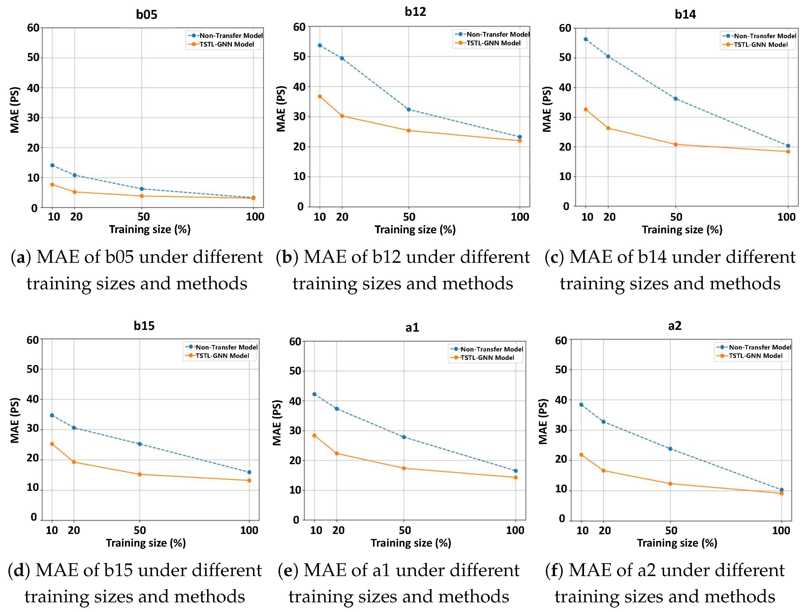
4.3. Path Delay Prediction Performance with Limited Data

One of the key advantages of transfer learning is the reduction in data requirements. In this experiment, we aim to prove the efficiency of TSTL-GNN model with limited data. We partitioned the training dataset into subsets of varying sizes: 10%, 20%, 50%, and 100%, maintaining a similar data distribution across all subsets, while keeping the test dataset unchanged. Comparing the results predicted by the TSTL-GNN model with those obtained from independently trained two-stage models. The results are illustrated in the example shown in Figure 4.

The results show that the TSTL-GNN model performs better when trained on a limited dataset compared to the non-transfer learning model. For most datasets, models using transfer learning exhibit lower MAE across all proportions of training data, indicating that transfer learning effectively reduces errors. Moreover, the advantage of transfer learning becomes more pronounced when the proportion of training data are smaller. As the proportion of training data increases, the MAE of models without transfer learning gradually decreases but still remains higher than that of models using transfer learning. The TSTL-GNN model leverages transfer learning to address data scarcity by supplementing delay prediction (target domain) data with transition time prediction (source domain) data. Even with less data, the TSTL-GNN model can achieve or approach the performance of a model trained from scratch with more data.

4.4. Path Delay Prediction for ECO in Typical Engineering Scenarios

To verify that the TSTL-GNN model has good generalization for netlists with ECO, we selected the benchmark b05 and performed some ECO operations on critical paths, such as changing cell types and inserting buffers. We trained the model on the original design and predicted the timing results of each path in the post-ECO netlists. We compared it with models without transition time prediction and evaluated the performance by using different models (GCN [29], GAT [30], GraphSage [31]). We also compared TSTL-GNN model with a previous work, GNN4REL [25]. The results are illustrated in the example shown in

Table 3. The accuracy of post-ECO netlist path delay prediction under various models ($R^2$ score/MAE). “POPC” stands for Percentage Of Path Change.

		b05	ECO1_b05	ECO2_b05	ECO3_b05	ECO4_b05	ECO5_b05	Average
ECO		-	Size cell	Size cell	Insert buffer	Insert buffer	Size cell+Insert buffer	-
POPC		-	5.32%	32.64%	10.79%	20.17%	52.43%	24.27%
GCN	$R^2$	0.7308	0.5242	0.3658	0.5575	0.2675	0.0891	0.3608
	MAE	51.37	128.45	199.82	106.81	258.63	576.81	254.10
GAT	$R^2$	0.6482	0.4765	0.4298	0.4367	0.2367	0.1067	0.3373
	MAE	65.13	136.79	187.62	119.20	309.58	489.28	248.49
GraphSAGE	$R^2$	0.9066	0.6612	0.5612	0.6941	0.4816	0.4014	0.5599
	MAE	9.41	65.34	92.78	60.31	115.97	147.97	96.47
GNN4REL	$R^2$	0.9618	0.8628	0.7651	0.8475	0.6542	0.5014	0.7262
	MAE	14.7	25.43	41.89	34.12	54.76	88.76	48.99
TSTL-GNN	$R^2$	0.9992	0.9362	0.9132	0.9593	0.9342	0.8985	0.9282
	MAE	3.11	6.38	14.12	5.62	12.64	20.69	11.89

.

The results show that:

• Compared to the prediction model without introducing transition time, the TSTL-GNN model has a significant improvement in scores for the second-stage prediction based on transfer learning, as it first performs a primary prediction for important features.
• For the netlists after different ECO operations, an average of 24.27% of paths have changed. The average prediction error of the TSTL-GNN model is 11.89 ps, which is better than traditional GNN methods. The stable $R^2$ score confirms our model’s good generalization. Meanwhile, compared to previous work, our model’s average prediction error has decreased by 37.1 ps after various ECO modifications.

4.5. Time Overhead of Path Delay Prediction

Once the path delay model is trained, extract the features of different input paths and make predictions. We report the prediction time of the TSTL-GNN model on a mixed dataset and compare it to the times from OpenSTA. The results are illustrated in the example shown in

Table 4. Run Time.

Benchmark	Runtime (s)
	Stage1	Stage2	Total	STA	Speedup
b05	3.6	2.2	5.8	38.6	6.66x
b12	4.2	2.6	6.8	52.8	7.76x
b14	4.4	2.8	7.2	92.9	12.9x
b15	5.5	3.1	8.6	121.7	14.15x
a1	12.9	8.5	21.4	1721.9	80.46x
a2	17.4	14.7	32.1	2460.7	76.65x
Average	8.0	5.7	13.7	748.1	54.61x

.

Compared to OpenSTA, our model achieves runtime improvement by up to 80 times, with particularly noticeable acceleration on large designs. For a single design, training the model only once enables the prediction of path delay after ECO, significantly reducing the time spent on timing analysis during iterations.

5. Conclusions

In this work, we introduce TSTL-GNN, a two-stage transfer learning approach using graph structures, which accurately predicts delay testing results of post-ECO modifications. The TSTL-GNN model aids designers in ECO analysis, simplifying ECO redesign and speeding up timing repair iterations. Our experiments show that, with 24.27% of paths modified, TSTL-GNN achieves a $R^{2}score/MAE$ of 0.9952/13.36. It surpasses traditional GNN and popular models by incorporating richer features, requiring less data, and enhancing model generalization through transfer learning, while also significantly saving time. Future work will focus on adding more relevant features and optimizing the graph structure.

References

1. Ho, K.H.; Jiang, J.H.R.; Chang, Y.W. TRECO: Dynamic technology remapping for timing engineering change orders. IEEE Trans. Comput.-Aided Des. Integr. Circuits Syst. 2012, 31, 1723–1733. [Google Scholar]
2. Huang, K.; Xiao, C.; Glass, L.M.; Zitnik, M.; Sun, J. SkipGNN: Predicting molecular interactions with skip-graph networks. Sci. Rep. 2020, 10, 21092. [Google Scholar] [CrossRef] [PubMed]
3. Yu, Y.; Qian, W.; Zhang, L.; Gao, R. A graph-neural-network-based social network recommendation algorithm using high-order neighbor information. Sensors 2022, 22, 7122. [Google Scholar] [CrossRef] [PubMed]
4. Davies, A.; Ajmeri, N. Realistic Synthetic Social Networks with Graph Neural Networks. arXiv 2022, arXiv:2212.07843. [Google Scholar]
5. Jiang, W.; Luo, J. Graph neural network for traffic forecasting: A survey. Expert Syst. Appl. 2022, 207, 117921. [Google Scholar] [CrossRef]
6. Tong, V.; Nguyen, D.Q.; Phung, D.; Nguyen, D.Q. Two-view graph neural networks for knowledge graph completion. In Proceedings of the European Semantic Web Conference, Crete, Greece, 28 May–1 June 2023; Springer: Berlin/Heidelberg, Germany, 2023; pp. 262–278. [Google Scholar]
7. Guo, Z.; Liu, M.; Gu, J.; Zhang, S.; Pan, D.Z.; Lin, Y. A Timing Engine Inspired Graph Neural Network Model for Pre-Routing Slack Prediction. In Proceedings of the 59th ACM/IEEE Design Automation Conference, DAC ’22, New York, NY, USA, 10–14 July 2022; pp. 1207–1212. [Google Scholar] [CrossRef]
8. Zhao, G.; Shamsi, K. Graph neural network based netlist operator detection under circuit rewriting. In Proceedings of the Great Lakes Symposium on VLSI 2022, Irvine, CA, USA, 6–8 June 2022; pp. 53–58. [Google Scholar]
9. Manu, D.; Huang, S.; Ding, C.; Yang, L. Co-exploration of graph neural network and network-on-chip design using automl. In Proceedings of the 2021 on Great Lakes Symposium on VLSI, Virtual, 22–25 June 2021; pp. 175–180. [Google Scholar]
10. Morsali, M.; Nazzal, M.; Khreishah, A.; Angizi, S. IMA-GNN: In-Memory Acceleration of Centralized and Decentralized Graph Neural Networks at the Edge. In Proceedings of the Great Lakes Symposium on VLSI 2023, Knoxville, TN, USA, 5–7 June 2023; pp. 3–8. [Google Scholar]
11. Lopera, D.S.; Servadei, L.; Kiprit, G.N.; Hazra, S.; Wille, R.; Ecker, W. A survey of graph neural networks for electronic design automation. In Proceedings of the 2021 ACM/IEEE 3rd Workshop on Machine Learning for CAD (MLCAD), Raleigh, NC, USA, 30 August–3 September 2021; pp. 1–6. [Google Scholar]
12. Ren, H.; Nath, S.; Zhang, Y.; Chen, H.; Liu, M. Why are Graph Neural Networks Effective for EDA Problems? In Proceedings of the 41st IEEE/ACM International Conference on Computer-Aided Design, San Diego, CA, USA, 30 October 2022–3 November 2022; pp. 1–8. [Google Scholar]
13. Pan, S.J.; Yang, Q. A Survey on Transfer Learning. IEEE Trans. Knowl. Data Eng. 2010, 22, 1345–1359. [Google Scholar] [CrossRef]
14. Wu, Z.; Savidis, I. Transfer Learning for Reuse of Analog Circuit Sizing Models Across Technology Nodes. In Proceedings of the 2022 IEEE International Symposium on Circuits and Systems (ISCAS), Austin, TX, USA, 27 May–1 June 2022. [Google Scholar] [CrossRef]
15. Chai, Z.; Zhao, Y.; Liu, W.; Lin, Y.; Wang, R.; Huang, R. CircuitNet: An Open-Source Dataset for Machine Learning in VLSI CAD Applications with Improved Domain-Specific Evaluation Metric and Learning Strategies. IEEE Trans. Comput. -Aided Des. Integr. Circuits Syst. 2023, 42, 5034–5047. [Google Scholar] [CrossRef]
16. Murray, K.E.; Betz, V. Tatum: Parallel Timing Analysis for Faster Design Cycles and Improved Optimization. In Proceedings of the 2018 International Conference on Field-Programmable Technology (FPT), Naha, Japan, 10–14 December 2018. [Google Scholar]
17. Yuasa, H.; Tsutsui, H.; Ochi, H.; Sato, T. Parallel Acceleration Scheme for Monte Carlo Based SSTA Using Generalized STA Processing Element. IEICE Trans. Electron. 2013, 96, 473–481. [Google Scholar] [CrossRef]
18. Huang, T.W.; Guo, G.; Lin, C.X.; Wong, M.D. OpenTimer v2: A New Parallel Incremental Timing Analysis Engine. IEEE Trans. Comput. -Aided Des. Integr. Circuits Syst. 2021, 40, 776–789. [Google Scholar] [CrossRef]
19. Guo, G.; Huang, T.W.; Wong, M. Fast STA Graph Partitioning Framework for Multi-GPU Acceleration. In Proceedings of the 2023 Design, Automation & Test in Europe Conference & Exhibition (DATE), Antwerp, Belgium, 17–19 April 2023; pp. 1–6. [Google Scholar] [CrossRef]
20. Guo, G.; Huang, T.W.; Lin, Y.; Guo, Z. A GPU-accelerated Framework for Path-based Timing Analysis. IEEE Trans. Comput.-Aided Des. Integr. Circuits Syst. 2023, 42, 4219–4232. [Google Scholar] [CrossRef]
21. Han, A.; Zhao, Z.; Feng, C.; Zhang, S. Stage-Based Path Delay Prediction with Customized Machine Learning Technique. In Proceedings of the 2021 5th International Conference on Electronic Information Technology and Computer Engineering, EITCE ’21, New York, NY, USA, 22–24 October 2022; pp. 926–933. [Google Scholar] [CrossRef]
22. Barboza, E.C.; Shukla, N.; Chen, Y.; Hu, J. Machine Learning-Based Pre-Routing Timing Prediction with Reduced Pessimism. In Proceedings of the the 56th Annual Design Automation Conference, Las Vegas, NV, USA, 2–6 June 2019. [Google Scholar]
23. Bian, S.; Shintani, M.; Hiromoto, M.; Sato, T. LSTA: Learning-Based Static Timing Analysis for High-Dimensional Correlated On-Chip Variations. In Proceedings of the Design Automation Conference, Austin, TX, USA, 18–22 June 2017. [Google Scholar]
24. Lopera, D.S.; Ecker, W. Applying GNNs to Timing Estimation at RTL. In Proceedings of the 41st IEEE/ACM International Conference on Computer-Aided Design, San Diego, CA, USA, 30 October–3 November 2022; pp. 1–8. [Google Scholar]
25. Alrahis, L.; Knechtel, J.; Klemme, F.; Amrouch, H.; Sinanoglu, O. GNN4REL: Graph Neural Networks for Predicting Circuit Reliability Degradation. IEEE Trans. Comput.-Aided Des. Integr. Circuits Syst. 2022, 41, 3826–3837. [Google Scholar] [CrossRef]
26. Yang, T.; He, G.; Cao, P. Pre-Routing Path Delay Estimation Based on Transformer and Residual Framework. In Proceedings of the 27th Asia and South Pacific Design Automation Conference (ASP-DAC), Taipei, Taiwan, 17 January 2022. [Google Scholar]
27. Guo, Z.; Lin, Y. Differentiable-Timing-Driven Global Placement. In Proceedings of the 59th ACM/IEEE Design Automation Conference, San Francisco, CA, USA, 10–14 July 2022. [Google Scholar]
28. Corno, F.; Reorda, M.S.; Squillero, G. RT-level ITC’99 benchmarks and first ATPG results. IEEE Des. Test Comput. 2000, 17, 44–53. [Google Scholar] [CrossRef]
29. Kipf, T.; Welling, M. Semi-Supervised Classification with Graph Convolutional Networks. arXiv 2016, arXiv:1609.02907. [Google Scholar]
30. Veličković, P.; Cucurull, G.; Casanova, A.; Romero, A.; Lio, P.; Bengio, Y. Graph attention networks. arXiv 2017, arXiv:1710.10903. [Google Scholar]
31. Hamilton, W.; Ying, Z.; Leskovec, J. Inductive Representation Learning on Large Graphs. In Proceedings of the Advances in Neural Information Processing Systems 30 (NIPS 2017), Long Beach, CA, USA, 4–9 December 2017. [Google Scholar]
Figure 1. The ECO process for critical paths.
Electronics 13 02897 g001
Figure 2. Framework of TSTL-GNN model.
Electronics 13 02897 g002
Figure 3. In the TSTL-GNN model training results, each scattered point depicts a path, the horizontal axis shows the ground-truth delay, the vertical axis displays the predicted delay, and the straight line represents the ideal result.
Electronics 13 02897 g003
Figure 4. MAE comparison between non-transfer learning model and TSTL-GNN model.
Electronics 13 02897 g004