Benchmarking Time-Frequency Representations of Phonocardiogram Signals for Classification of Valvular Heart Diseases Using Deep Features and Machine Learning

Abstract

Heart sounds and murmur provide crucial diagnosis information for valvular heart diseases (VHD). A phonocardiogram (PCG) combined with modern digital processing techniques provides a complementary tool for clinicians. This article proposes a benchmark different time–frequency representations, which are spectograms, mel-spectograms and cochleagrams for obtaining images, in addition to the use of two interpolation techniques to improve the quality of the images, which are bicubic and Lanczos. Deep features are extracted from a pretrained model called VGG16, and for feature reduction, the Boruta algorithm is applied. To evaluate the models and obtain more precise results, nested cross-validation is used. The best results achieved in this study were for the cochleagram with 99.2% accuracy and mel-spectogram representation with the bicubic interpolation technique, which reached 99.4% accuracy, both having a support vector machine (SVM) as a classifier algorithm. Overall, this study highlights the potential of time–frequency representations of PCG signals combined with modern digital processing techniques and machine learning algorithms for accurate diagnosis of VHD.

1. Introduction

Cardiovascular disorders (CVD) and valvular heart diseases (VHD) are the leading cause of mortality worldwide [1]. Recent studies have shown that AI capabilities have potential for health monitoring; automation of these tasks could free up clinicians for more complex work and improve access to health care [2]. Heart sound classification is an essential task for diagnosing and monitoring heart conditions.

VHD is a growing public health problem that should be addressed with appropriate resources to improve diagnosis and treatment [3]. Aortic stenosis (AS) is the most recurrent valvular disorder in developed countries (affecting 9 million people worldwide) [4], and its prevalence is increasing with the aging of the population and the increasing prevalence of atherosclerosis, and it is characterized by a harsh, systolic ejection murmur that is best heard at the right upper sternal border [5]. Mitral regurgitation (MI) is one of the most common heart valve disorders worldwide, with an estimated prevalence of 1.7% [6], and it is characterized by a holosystolic murmur that is best heard at the apex and radiates to the axilla. Mitral stenosis (MS) is a common disease that causes a large number of diseases throughout the world. This disease is more recurrent in developing countries, but in developed countries it is becoming more common in atypical forms [7], and it is characterized by a low-pitched, diastolic rumble that is best heard at the apex with the patient in the left lateral decubitus position. Mitral valve prolapse (MVP) is a frequent condition that affects 2–3% of the general population, and it is characterized by a mid-to-late systolic click followed by a late systolic murmur that is best heard at the apex and radiates to the axilla [3,8]. These are common heart valve disorders with distinct characteristics and prevalences worldwide, and each condition has a unique auscultation finding that helps in diagnosis.

Phonocardiography (PCG) is a diagnostic technique that analyzes heart sounds acquired at the chest wall to determine if the heart is functioning normally or if further diagnosis is required. Skilled cardiologists typically analyze these sounds, which result from muscle contractions and heart valve closure. However, this process can be affected by factors such as environmental noise, limitations in audible frequency range and the medical examiner’s expertise [9,10]. Given these problems, solutions have been developed over the last few years to help provide a better diagnosis, aided by technology for the analysis and classification. Based on previous work, we can highlight three stages for the classification of PCG signals: preprocessing, feature extraction and classification. Spectrograms, mel-spectrograms and Cochleograms are time–frequency multi-representations that provide a way to visualize the frequency content of PCG signals over time. Each method has unique characteristics and limitations. Spectrogram uses a Fourier transform to convert a signal from the time domain to the frequency domain [11]. Spectrograms are widely used due to their straightforward implementation and interpretation. They provide a clear view of how frequencies change over time but suffer from a trade-off between time and frequency resolution, which can limit their effectiveness in analyzing rapidly changing signals. Mel-spectrograms use a mel-scale filterbank to approximate the nonlinear human auditory system [12]. Mel-spectrograms are particularly effective for tasks related to human perception of sound, as they reflect the human ear’s sensitivity to different frequencies. However, the nonlinear transformation can sometimes obscure fine details in the frequency content, potentially limiting its use in precise scientific analyses. Cochleogram is a time–frequency representation (TFR) that simulates the cochlea in the inner ear, responsible for frequency analysis in the auditory system [13,14]. This method provides a biologically inspired approach to analyzing signals, offering insight into how humans perceive sound. However, its complexity can be a limitation, requiring more computational resources and potentially being less intuitive for those unfamiliar with biological signal processing. The use of bicubic and Lanczos interpolation methods for resizing the time–frequency representations is a significant contribution to this work [5,15]. These methods ensure the preservation of the original signal’s quality while providing uniform input dimensions for the classification models. By employing these high-quality resizing techniques, the performance and robustness of the classification models are enhanced, facilitating more accurate diagnosis and monitoring of valvular heart diseases.

The preprocessing, studies have been carried out for segmented signals as in [16] the segmentation is performed synchronously and asynchronously with different sizes. The Shannon energy envelope and zero crossing is a proposed algorithm for segmentation [17]. In this work, we will not use signal segmentation, since we may lose information from the signals.

The conventional methods of heart sound signal feature extraction, like time domain, are as in [18], where the authors extract 12 features and to reduce them use feature reduction techniques, matching pursuit time–frequency decomposition using Gabor dictionaries [19]. hort-time Fourier transform (STFT)-based spectrograms represent patterns of the normal and abnormal PCG signals [20]. In [21], the authors use discrete wavelet transform (DWT) to extract features, continued with wavelet transform-based spectrograms (CWTS) [22], Hilbert–Huang transform (HHT) [23] and Mel-frequency cepstral coefficients (MFCC) [12,24]. Since the extraction of characteristics may not be as efficient manually, it is proposed to use pretrained neural networks such as Alexnet, VGG16 and VGG19 to extract deep features [10,24].

In the last stage, many types of machine learning for the classification of PCG signals to detect different types of CVD have been proposed, such as a one-dimensional deep neural network (1-D DNN) with low parameters to detect abnormalities of Cardiovascular disease [25]. In [26], the authors propose a combination of CNN and bidirectional long short-term memory (CNN-BiLSTM). In [27], they used five different types of artificial neural network (ANN), named narrow, wide, tri-layered, bi-layered and medium. In [28], the residual neural network (Resnet) was used to avoid losing information from the previous layers.

Table 1. A comparative performance of existing work for cardiac disease classification.

Authors	Database	Classes	Feature Extraction	Classifier	Accuracy
Yaseen et al. [18]	Yanseen Database	Five	MFCCs + DWT	SVM	97.9%
O. Arslan [10]	Yanseen Database	Five	Features-based ML-ELM + RFE feature selection	Random forest	98.9%
Q. Abbas et al. [19]	Yanseen Database	Five	CWT + spectogram	CVT + ATTF	99%
S. Das et al. [7]	Physionet/Cinc Database	Two	Cochleagram	DNN	98.3%
K. Ghosh et al. [3]	Yanseen Database	Five	LEN and LENT- based features using CT	Multiclass composite	99.4%

shows the different techniques of feature extraction performance with the classifiers used by the authors, where we can see the types of two-class and five-class classifications of PCG signals.

In this study, we present a benchmark of heart sound classification systems based on time–frequency multi-representations. The goal of this benchmark is to provide a comprehensive comparison of state-of-the-art heart sound classification systems and to identify the most effective TFR for detecting valvular heart diseases. The other contributions of this work are summarized in the following points:

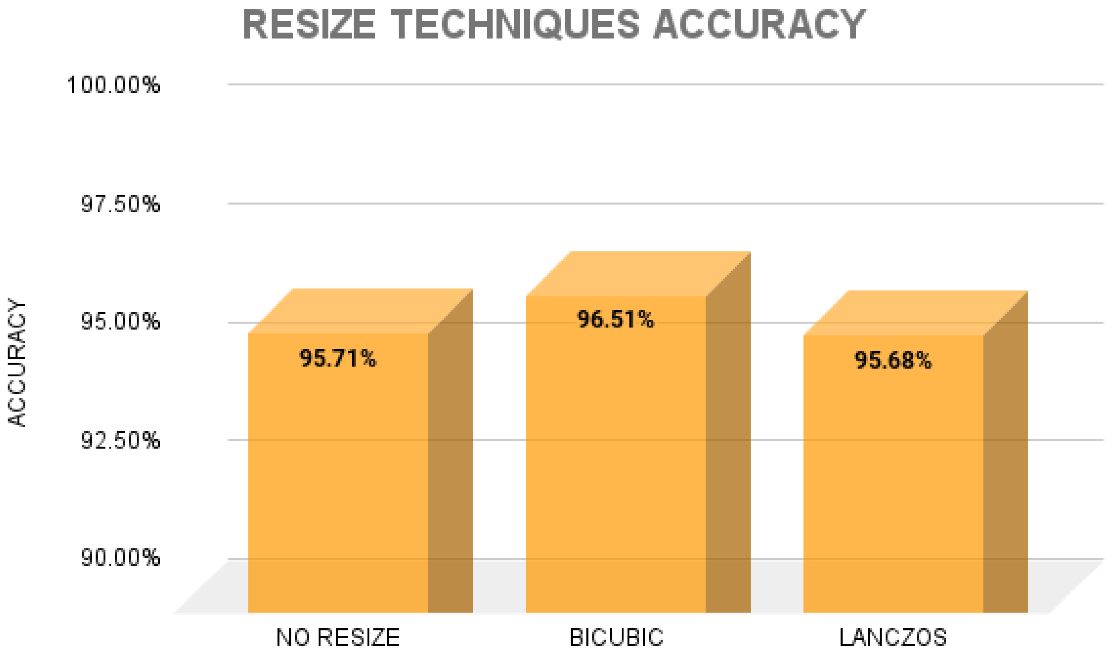
• Employing resizing techniques to TFRs to improve sorting performance.
• The use of the Boruta feature selector to narrow down the features to the most important ones.
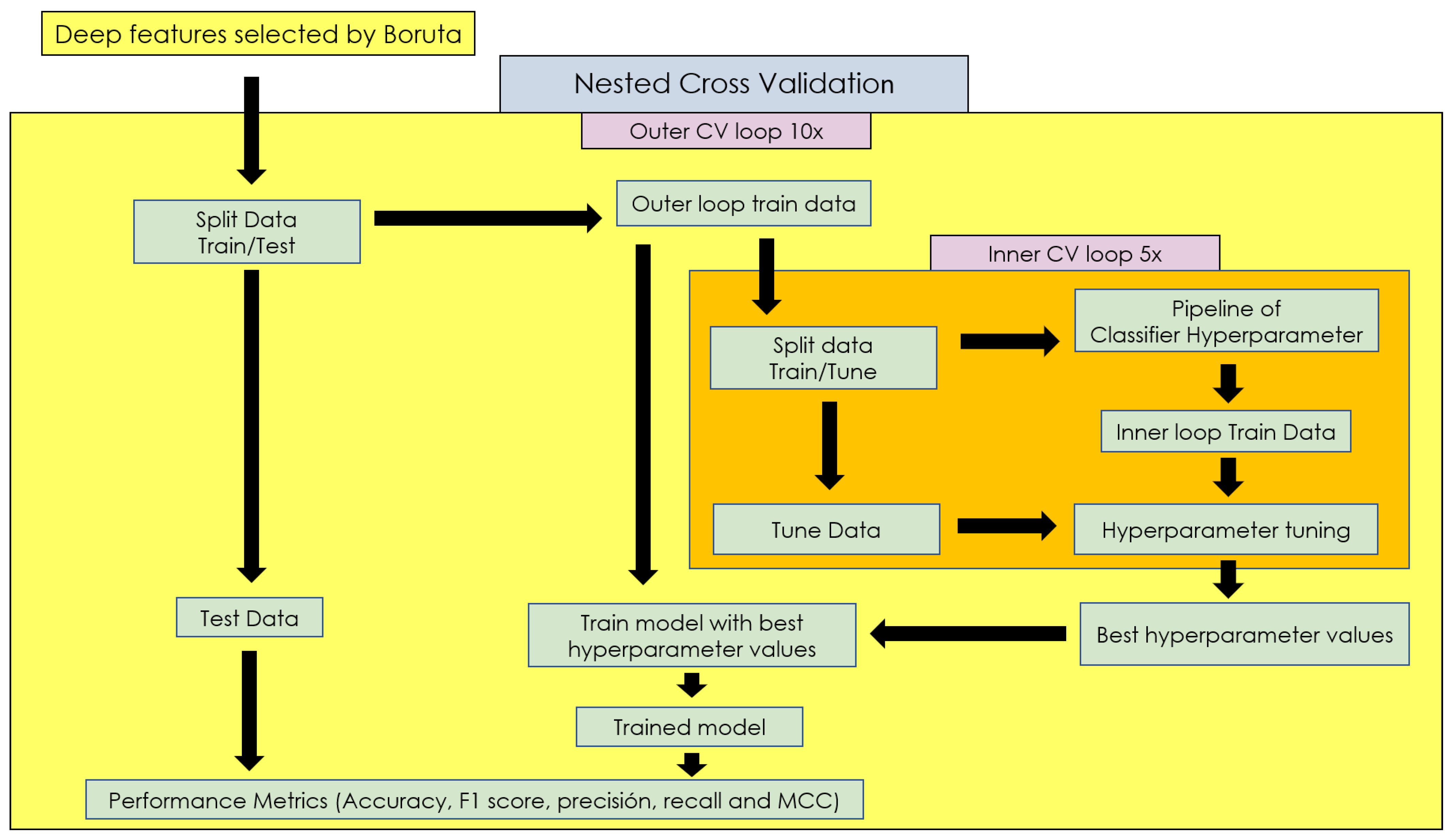
• Performing a nested cross-validation (nCV) approach that combines cross-validation with an additional model selection process.
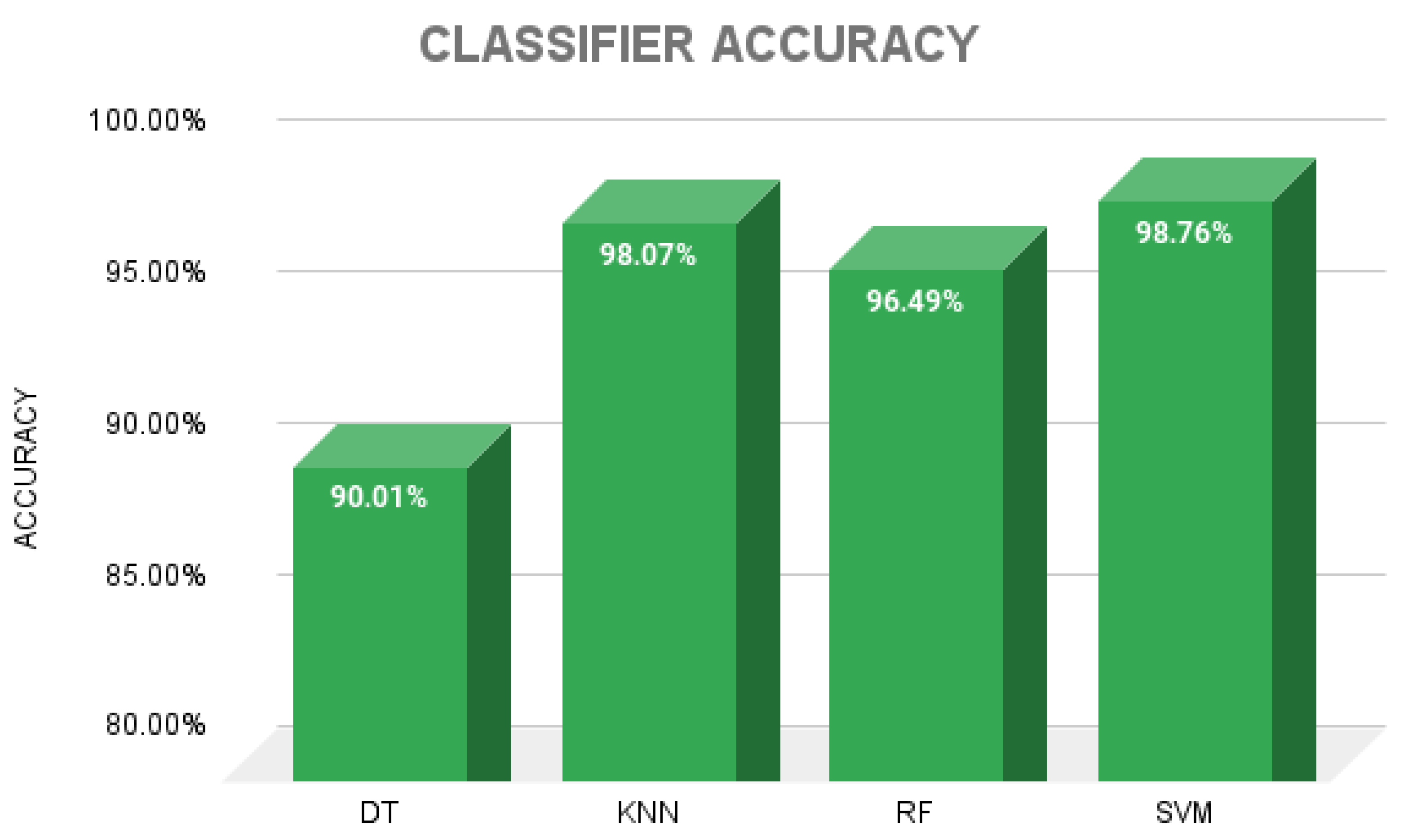
• Comparison of the classification performance of machine learning algorithms such as decision trees (DTs), K-nearest neighbors (KNN), random forests (RF) and support vector machines (SVM).

This paper is part of the research development in the area of biomedical engineering of the Universidad Nacional de San Agustin de Arequipa [29,30,31,32] for the Think Health project, which seeks to improve medical assistance in the auscultation process.

2. Materials and Methods

2.1. Dataset

The heart sound database was acquired from an open-source dataset made by Yanseen [21]. In

Table 2. Table of heart disease sound files and sample sampling rate.

Valve Heart Disease	Files (Wav.) Amount	Sample Frequency (Hz)
Aortic Stenosis (AS)	200	8000
Mitral Regurgitation (MR)	200	8000
Mitral Stenosis (MS)	200	8000
Mitral Valve Prolapse (MVP)	200	8000
Normal (N)	200	8000

, the database consists of a total of 1000 heart sound recordings (800 abnormal and 200 normal), gathered from various sources, sampled at a frequency of 8000 Hz. There are 5 classes: aortic stenosis (AS), mitral regurgitation (MR), mitral stenosis (MS), mitral valve prolapse (MVP) and normal (N), with each class having 200 recordings.

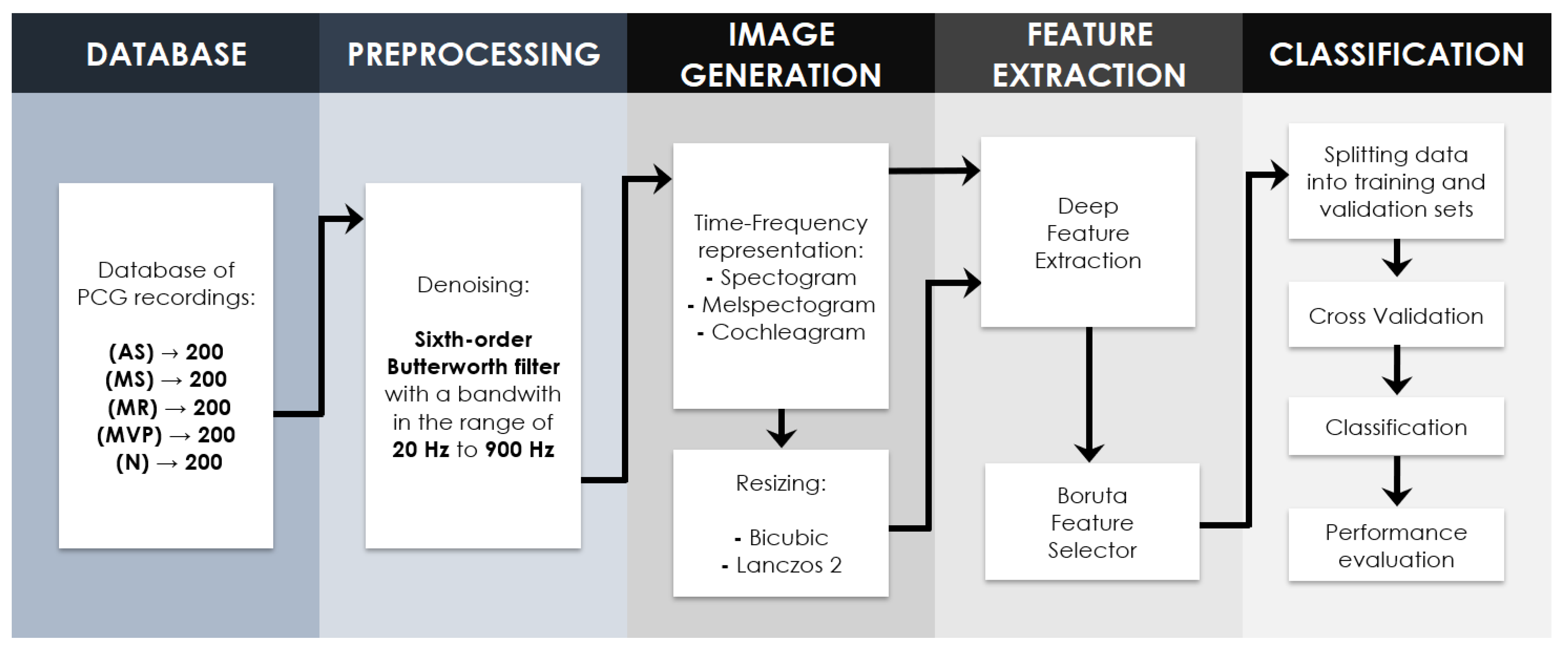
2.2. Proposed Methodology

This study proposes the use of various time–frequency representations (TFR), including spectrograms, mel-spectrograms and cochleograms, to improve the accuracy of heart sound classification systems. The aim is to evaluate the performance of these different TFR methods in a comparative study with previous works.

To accomplish this in Figure 1 a dataset of heart sound recordings is collected and labeled for classification. The dataset consists of recordings from different patients, with various heart conditions, and collected from different sources. The heart sound signals are preprocessed to remove noise and artifacts. The output PCG filtered are then transformed into different time–frequency representations using the selected TFR methods.

In the next step, different classification algorithms are trained and tested using the dataset and the TFR methods. The algorithms include traditional machine learning methods, such as support vector machines (SVM) and random forests (RF), decision trees (DT) and K-nearest neighbors (KNN), as well as deep learning methods, such as convolutional neural networks (CNN). The performance of each algorithm is evaluated using standard evaluation metrics, such as accuracy, precision, MCC (Matthews correlation coefficient), recall and F1-score.

Finally, a comparative analysis is performed to determine the effectiveness of each TFR method in improving the accuracy of heart sound classification. The analysis includes a comparison of the performance of the different algorithms using each TFR method. The results of the study can be used to guide the development of more accurate and efficient heart sound classification systems, with the potential to improve the diagnosis and treatment of heart disease.

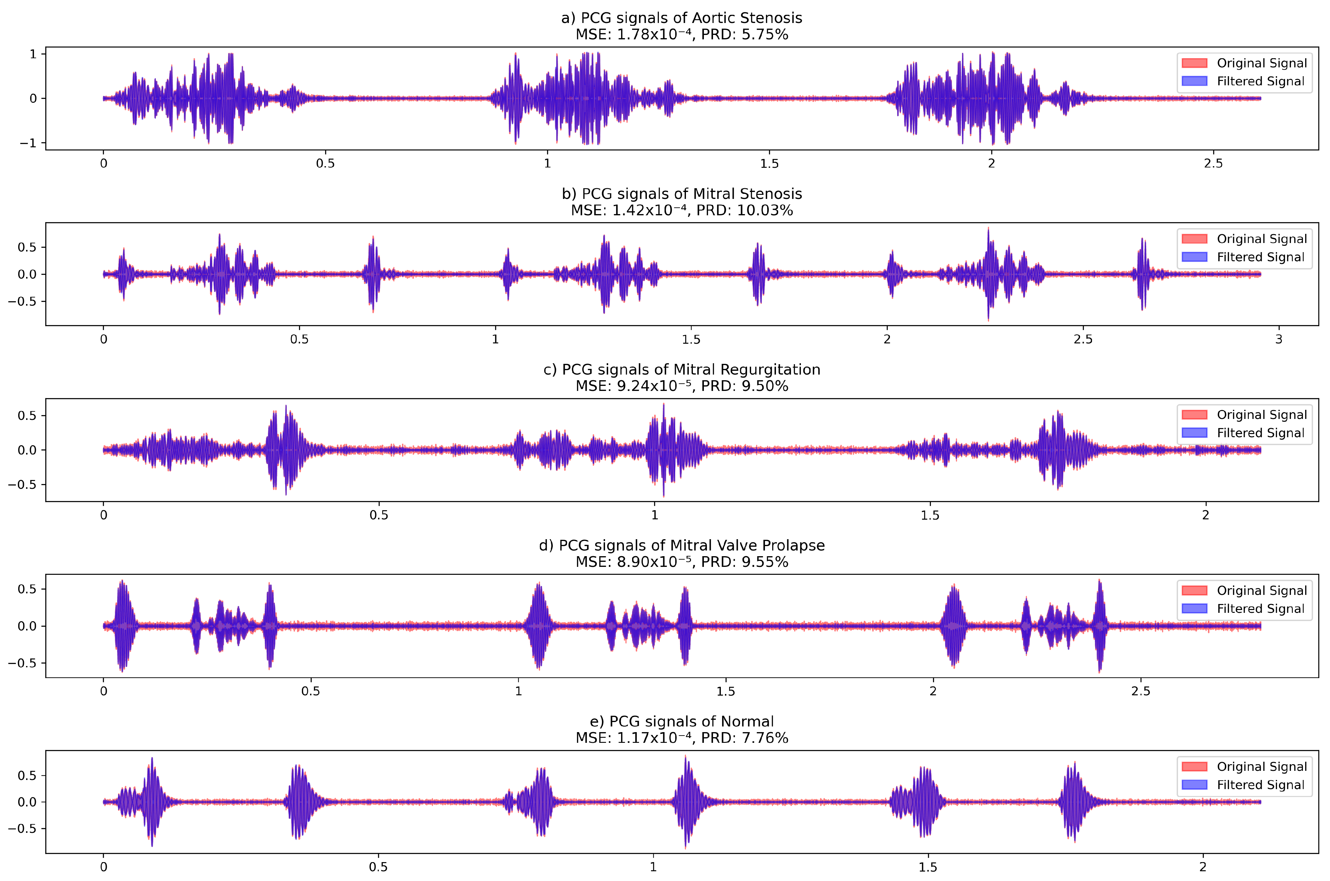
2.2.1. Signal Preprocessing

A Butterworth filter is an essential signal processing tool used for smoothing frequency responses and attenuating noise in various types of signals, including audio and biomedical data. In the case of processing these PCG files, a sixth-order Butterworth filter with a passband of 20 Hz to 900 Hz can be highly effective in isolating heart sounds while minimizing external noise and artifacts as shown in Figure 2. This specific filter order and bandwidth selection is crucial for maintaining the integrity of the original signal while reducing unwanted frequency components, as higher-order Butterworth filters exhibit a steeper roll-off rate and a flatter response in the passband. PCG signals are subject to several sources of noise that interfere with data quality and make accurate analysis of heart sounds difficult. Low-frequency noises, such as breathing and body movements, can introduce artifacts that distort the heart signal. These noises are usually below 20 Hz and originate from the patient’s breathing and body movements, which can overlap essential heart sounds and complicate their identification. On the other hand, high-frequency noises, which exceed 900 Hz, come from sources such as muscle contractions and electrical interference from nearby devices. These high-frequency noises can mask the fine details of heart sounds, making it difficult to analyze the signal in detail and accurately [33]. The application of a sixth-order Butterworth filter with a 20 Hz to 900 Hz passband is a well-established technique in the literature for extracting valuable diagnostic information from PCG signals, enabling healthcare professionals to analyze heart sounds and identify potential abnormalities more accurately.

The following

Table 3. Comparison of MSE and PRD for denoised signals.

Signal	MSE	PRD (%)
Aortic Stenosis	0.000282	5.75
Mitral Stenosis	0.000246	10.03
Mitral Regurgitation	0.000199	9.50
Mitral Valve Prolapse	0.000186	9.55
Normal	0.000218	7.76

provides a comparison of the denoising performance using MSE and PRD metrics for different types of pathological heart sounds and normal heart sounds. Lower MSE and PRD values indicate better denoising performance.

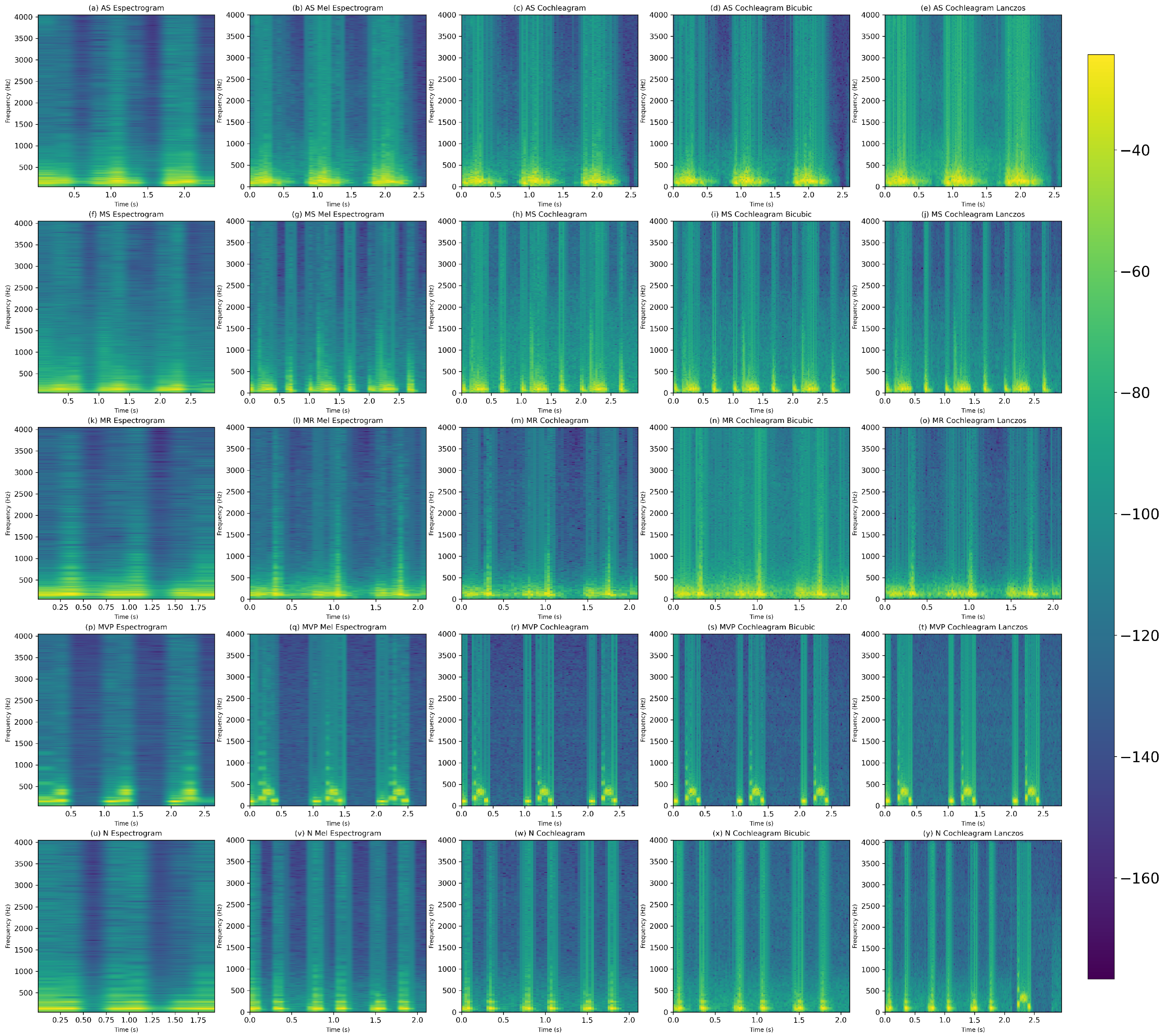
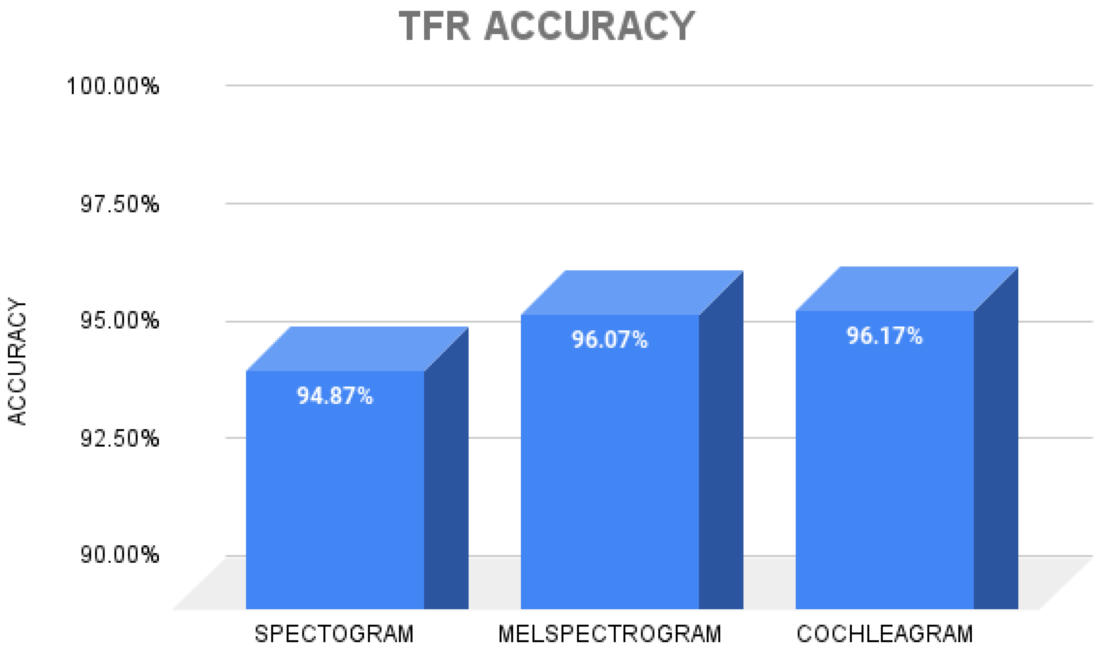
2.3. Time–Frequency Representations

2.3.1. Spectrogram

The spectrogram serves as a valuable analytical tool for examining signals like the phonocardiogram, facilitating the visual depiction of energy distribution across various frequencies over time. Mathematically, the spectrogram is derived through [34] the continuous short-time Fourier transform (STFT), expressed as

$$S(f,t)={\int }_{-\infty }^{\infty }x\left(\tau \right)w(\tau -t)e^{-j2\pi f\tau }d\tau$$

(1)

In this equation, $S(f,t)$ denotes the spectrogram value at frequency f and time t. The function $x\left(\tau \right)$ represents the input signal, whereas $w(\tau -t)$ signifies an analysis window utilized to constrain the signal’s influence over a time interval centered around t. The component $e^{-j2\pi f\tau }$ embodies a complex exponential function contingent upon frequency f and time $\tau$.

The computation of the spectrogram involves the evaluation of this integral across diverse f and t values, furnishing an intricate portrayal of energy distribution within the time-frequency realm. This method is particularly advantageous for discerning temporal variations within the signal, a capability of paramount importance in the diagnosis of cardiac ailments such as valvular heart diseases.

2.3.2. Mel-Spectogram

The mel-spectrogram, akin to the conventional spectrogram, is a crucial tool in signal analysis, especially in domains like phonocardiography. It provides a detailed representation of signal energy distributed across frequencies over time, with a perceptually relevant frequency scale. Mathematically, the mel-spectrogram is computed by first transforming the signal into the mel-frequency domain, followed by calculating the spectrogram using a mel filterbank.

The transformation into the mel-frequency domain involves mapping the linear frequency scale (in Hertz) into the mel scale, which is perceptually linear [35]. This mapping is typically achieved using the formula

$$M\left(f\right)=2595·ln(1+{\displaystyle \frac{f}{700}})$$

(2)

Here, $M\left(f\right)$ represents the mel-frequency corresponding to the linear frequency f.

After the signal is transformed into the mel-frequency domain, the spectrogram is computed using a mel filterbank. This involves applying a set of triangular filters, equally spaced in mel-frequency, to the mel-scaled signal. The energy within each filterbank is then calculated, resulting in the mel-spectrogram.

The mel-spectrogram provides a perceptually relevant representation of signal characteristics, making it particularly useful for tasks such as speech and audio processing. In the context of diagnosing conditions like valvular heart diseases, the mel-spectrogram can offer valuable insights into the temporal and spectral features of phonocardiographic signals, aiding in accurate diagnosis and analysis.

2.3.3. Cochleagram

The cochleagram is a specialized representation of auditory signals, particularly useful in analyzing phonocardiographic data. It mimics the processing that occurs in the human auditory system, providing a representation of signal energy that is sensitive to both frequency and time, akin to the functioning of the cochlea in the ear.

Mathematically, the cochleagram is computed by passing the signal through a bank of filters resembling the frequency response of the human cochlea. These filters are typically spaced on a logarithmic frequency scale to emulate the tonotopic organization of the cochlea. The signal’s energy within each filter is then computed, yielding a time–frequency representation akin to the human auditory system’s response to sound.

The cochleagram computation involves several steps, beginning with the construction of the filterbank [14]. Each filter’s response is designed to mimic the frequency selectivity of the corresponding region in the cochlea. The signal is then convolved with each filter in the bank, and the resulting energies are computed over time, yielding the cochleagram representation.

The cochleagram is mathematically expressed as

$$C(f,t)=\sum _{k=1}^N{|x\left(t\right)\ast h_k\left(t\right)|}^2$$

(3)

where $C(f,t)$ denotes the cochleagram value at frequency f and time t, $x\left(t\right)$ represents the input signal, and $h_k\left(t\right)$ represents the impulse response of the k-th cochlear filter in the bank. The sum is computed over all N filters in the cochlear filterbank.

The cochleagram offers a perceptually relevant representation of auditory signals, capturing both temporal and spectral features. In the context of diagnosing conditions like valvular heart diseases, the cochleagram can provide valuable insights into the acoustic characteristics of phonocardiographic signals, facilitating accurate diagnosis and analysis.

2.4. Resizing Image Techniques

The resize technique is an important component of audio signal processing, which allows us to adjust the size of the spectrogram, mel-spectrogram and cochleagram representations. Two commonly used resize techniques are Lanczos and bicubic [36]. The Lanczos resize technique provides a smoother resizing operation, which can help to preserve the quality of the original signal. The bicubic resize technique provides a sharper resizing operation, which can help to enhance the detail of the signal. In Figure 3, both resize techniques are shown to improve the performance of various audio classification tasks, including speech recognition and music genre classification.

2.4.1. Bicubic

Bicubic interpolation is a method commonly employed for resizing digital images, offering smoother transitions and reduced artifacts compared to linear interpolation techniques [37]. It involves fitting a cubic polynomial to a 4x4 neighborhood of pixels surrounding each output pixel, allowing for more flexible and accurate estimation of pixel values.

2.4.2. Lanczos

Lanczos interpolation, on the other hand, is a resampling technique that aims to maintain image fidelity while reducing aliasing artifacts [38]. It utilizes a windowed sinc function to interpolate pixel values, providing high-quality results particularly suited for applications where preserving image details is crucial. The Lanczos kernel is defined as

$$L\left(x\right)=\left\{\begin{array}{cc}\mathrm{sinc}\left(x\right)·\mathrm{sinc}\left({\displaystyle \frac{x}{4}}\right),\hfill & \mathrm{if}\left|x\right|<4\hfill \\ 0,\hfill & \mathrm{otherwise}\hfill \end{array}\right.$$

(4)

In this equation, $\mathrm{sinc}\left(x\right)={\displaystyle \frac{sin\left(\pi x\right)}{\pi x}}$ represents the sinc function, and x is the distance from the center of the kernel. Lanczos interpolation involves convolving the input image with this kernel, centered at the target pixel location, to compute the interpolated pixel value.

In Figure 3, shows multiple time–frequency representations of a few samples. This figure shows the differences between each image by applying the different methods previously shown; it can also be seen in

Table 4. MSE and PSNR comparison of some TFR.

TFR Type	Spect		Mel Spect		Coch		Coch-B		Coch-L
	MSE	PSNR	MSE	PSNR	MSE	PSNR	MSE	PSNR	MSE	PSNR
AS	0.0012	49.50	0.0010	49.70	0.0009	49.80	0.0008	50.10	0.0007	50.20
MS	0.0011	49.60	0.0010	49.80	0.0009	49.90	0.0007	50.30	0.0006	50.40
MR	0.0008	49.90	0.0007	50.00	0.0006	50.10	0.0005	50.50	0.0004	50.60
MVP	0.0009	49.80	0.0008	49.90	0.0007	50.00	0.0006	50.40	0.0005	50.50
N	0.0007	50.00	0.0006	50.10	0.0005	50.20	0.0004	50.60	0.0004	50.50

that the MSE and PSNR factor look like good parameters since by making changes in the image in postprocessing, it can affect the quality of the same time to use it for classification, but we see that this is not shown in the table.

The PCG signal, capturing heart sounds, undergoes transformation into images using frequency and time representation techniques such as spectrograms, mel-spectrograms, and cochleagrams. These transformations exhibit distinct visual patterns corresponding to different cardiac conditions, specifically aortic stenosis (AS), mitral stenosis (MS), mitral regurgitation (MR), mitral valve prolapse (MVP) and normal (N). For example, AS images might show an increase in high frequencies due to aortic valve obstruction, while MS images may display specific frequency patterns associated with mitral valve flow restriction. MR images could reveal anomalous frequencies related to retrograde flow through the mitral valve, and MVP images may exhibit variations in frequency and duration of heart sounds due to mitral valve dysfunction. In contrast, images representing normal conditions would display characteristic patterns of regular and well-defined heart sounds at usual frequencies. These visual representations provide valuable insights into differences in heart sounds among various cardiac conditions, facilitating diagnosis and disease monitoring.

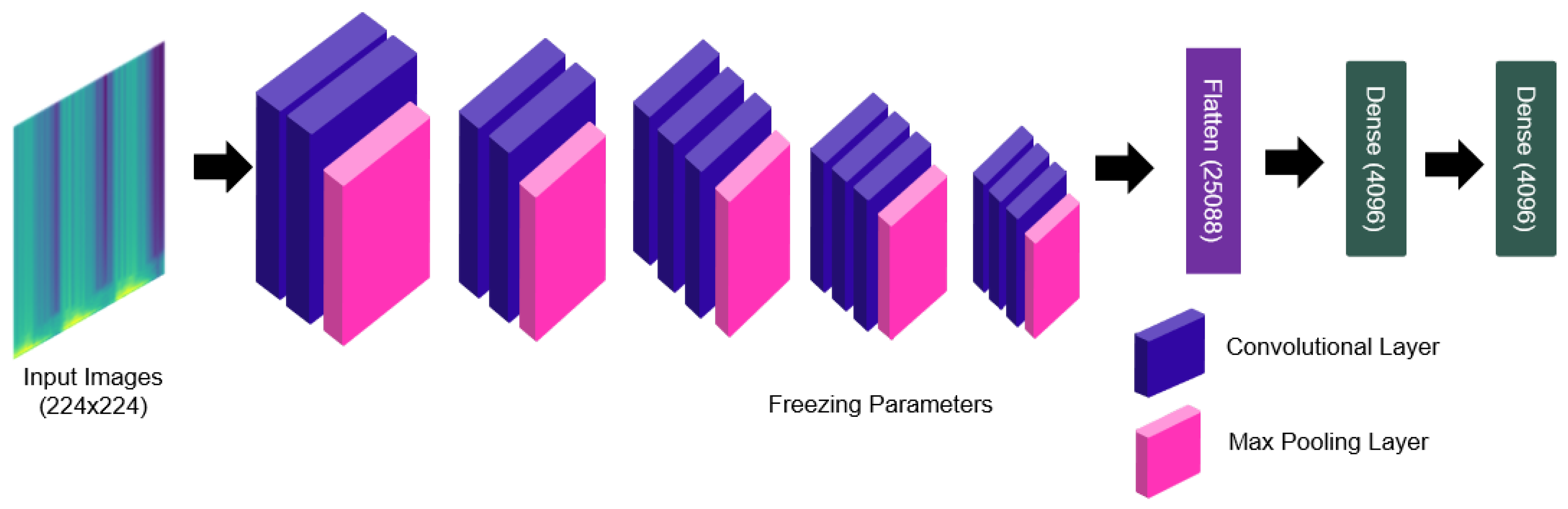
2.4.3. Deep Feature Extraction

There are many pretrained models that were trained with one of the largest datasets of image recognition called ImageNet. In previous studies [28,33], they made use of different pretrained models for deep feature extraction. In this study, we take one of those models, called VGG16, and change it from a classifier to a feature extractor for the different TFRs and their respective resize techniques.

In Figure 4 illustrates the modified structure of the VGG16: The images must have a size of 224 × 224. Following the structure of the model, we have thirteen convolutional layers and five max-pooling layers; after the last max-pooling layer, we have a flattened layer to reduce the dimensions of the output, and then we added two fully connected layers. The model operates with 134 million parameters. At the output of the model, we will have a vector of 4096 characteristics or deep features of each class of images that will serve as input for the classification algorithms.

2.4.4. Boruta Feature Selection Algorithm

As shown in previous studies [39], the selection of features increases the performance of the classification algorithms because some features may be redundant or unnecessary. In this work, we use the Boruta algorithm to perform feature selection, which works in conjunction with the random forest algorithm [40]; more information about the steps of the Boruta algorithm can be found in [41].

2.4.5. Nested Cross-Validation

Nested cross-validation is a technique used to robustly and objectively evaluate and select models. In this approach, multiple cross-validation iterations are performed: an external one to evaluate the performance of the model and an internal one to tune the model hyperparameters. Outer cross-validation is responsible for evaluating the performance of the final selected model, while inner cross-validation is used to select the best hyperparameters of the model. This approach provides a more reliable assessment of model performance because it avoids the overfitting of test data and ensures the correct selection of hyperparameters [42].

In this case, we use this type of cross-validation because we have a large number of characteristics for the analysis; therefore, given the number of classification algorithms, it is necessary to have the best parameters of each of them so that better results can be obtained. Optimal Figure 5 explains how our NCV (nested cross-validation) works, composed of an inner loop and an outer loop. For the first case, a hyperparameter adjustment is made for each of the classifiers with already pre-established characteristics. This procedure is carried out as follows: 5-fold cross-validation so that with the best characteristics of each classifier, we move to the outer loop, where here each classification model is trained with 10-fold cross-validation, randomly distributing the testing and training data and then at the end being evaluated with the corresponding metrics such as accuracy, F1-score, precision, recall and Matthews correlation coefficient (MCC).

2.4.6. Classifiers

Given that there is no absolute classification algorithm that will always perform best in any given situation, this paper uses several models of classification algorithms to evaluate the performance of each algorithm and obtain a general idea of which algorithm is better for each type of input. We propose the use of four classification algorithms, which are decision trees (DTs) [43], K-nearest neighbors (KNN) [44], random forests (RF) [45] and support vector machines (SVM) [46].

2.4.7. Performance Evaluation Metrics

In assessing the outcomes of this study, we employed five distinct metrics for evaluation: accuracy ($Acc$), precision ($Pre$), recall ($Rec$), F1-score ($F1$), and Matthews correlation coefficient ($MCC$). These metrics provide various insights into the performance of each model and are calculated as follows:

$$Acc={\displaystyle \frac{Tp+Tn}{Tp+Tn+Fp+Fn}}$$

(5)

$$Pre={\displaystyle \frac{Tp}{Tp+Fp}}$$

(6)

$$Rec={\displaystyle \frac{Tp}{Tp+Fn}}$$

(7)

$$F1={\displaystyle \frac{2\ast Pre\ast Rec}{Pre+Rec}}$$

(8)

$$MCC={\displaystyle \frac{Tp\ast Tn-Fp\ast Fn}{\sqrt{(Tp+Fp)(Tp+Fn)(Tn+Fp)(Tn+Fn)}}}$$

(9)

True positive ($TP$) signifies the count of correctly classified instances where diseased PCGs were correctly identified as diseased. False positive ($FP$) represents instances where diseased PCGs were incorrectly classified as healthy. True negative ($TN$) corresponds to instances where healthy PCGs were accurately classified as healthy. Finally, false negative ($FN$) indicates instances where healthy PCGs were mistakenly classified as diseased.

In essence, $TP$ and $TN$ reflect correct classifications, while $FP$ and $FN$ indicate misclassifications. $TP$ and $TN$ capture instances where the classifier’s prediction aligns with the true status of the VHDs, whereas $FP$ and $FN$ illustrate cases where the classifier’s prediction deviates from the true status.

3. Results

The diagnosis of cardio-valvular diseases is a complex issue since the signals are not always obtained cleanly, which is why, as explained in Section 2.2.1, preprocessing is performed for each type of signal that was used in this work. In the next stage, the TFRs obtained from PCG signals of VHDs were given as input for the pretrained VGG16 model and given the large number of these obtained.

Table 5. Boruta algorithm performance with 10 iterations.

TFRs	Resize Technique	Confirmed	Tentative	Rejected
Spectogram	-	1028	272	2796
Spectogram	Bicubic	1031	154	2911
Spectogram	Lanczos	959	198	2939
Mel-spectogram	-	1007	394	2695
Mel-spectogram	Bicubic	936	337	2823
Mel-spectogram	Lanczos	980	300	2816
Cochleagram	-	1130	400	2566
Cochleagram	Bicubic	1142	398	2556
Cochleagram	Lanczos	1124	410	2562

shows the features confirmed, tentative and rejected for each type of TFR. The number of iterations performed for the selection was 10. The last part consisted of an nCV to obtain the best parameters of each classifier for each type of given input and obtain a correct classification. For this research, a machine with 16 GB of RAM Kingston, Ryzen 5 3600 processor and an NVIDIA GeForce RTX 3060 video card was used. Obtaining characteristics, as well as training each model, was carried out in the Spyder 4.1.4 software using Python 3.7.7 with the libraries Tensorflow 2.12.0 and Tensorflow-GPU 2.10.0.

As previously indicated, this work seeks alternative ways of extracting features in order to improve the classification performance. Firstly, as we see in

Table 6. Results for TFRs.

Methods/Algorithm	Performances (%) for Confirmed Features
	$\mathit{Pre}$	$\mathit{Rec}$	$\mathit{F}\mathbf{1}$	$\mathit{MCC}$	$\mathit{Acc}$
Spec/DT	86.36	86.30	86.31	82.88	86.20
Spec/KNN	96.71	96.70	96.70	95.87	96.70
Spec/RF	94.95	94.90	94.88	93.64	94.90
Spec/SVM	97.51	97.50	97.49	96.88	97.50
Mel/DT	91.50	91.50	91.47	89.39	91.50
Mel/KNN	97.95	97.90	97.89	97.39	97.90
Mel/RF	95.55	95.55	95.47	94.40	95.50
Mel/SVM	98.90	98.90	98.89	98.62	98.90
Coch/DT	91.04	91.00	91.01	88.75	91.00
Coch/KNN	98.61	98.60	98.59	98.25	98.60
Coch/RF	97.52	97.50	97.49	96.88	97.50
Coch/SVM	99.20	99.20	99.19	99.00	99.20

, different TFRs were used but without applying resize techniques, where initially, a quantity of 4096 deep features was obtained. By then applying Boruta feature selection, confirmed deep features were obtained: 1028 for the spectogram, 1007 for the mel-spectogram and 1130 for the Cochleagram, as shown in Table 5. The highest performance values were obtained using the cochleagram and SVM as the classifier, with the values of 99.2% precision, 99.2% recall, 99.19% F1 score, 99% Matthews correlation coefficient and 99.2% accuracy.

Another objective of this work was to apply resize techniques for the TFRs, where in this case, as shown in

Table 7. Results for TFRs with bicubic resize technique.

Methods/Algorithm	Performances (%) for Confirmed Features
	$\mathit{Pre}$	$\mathit{Rec}$	$\mathit{F}\mathbf{1}$	$\mathit{MCC}$	$\mathit{Acc}$
Spec + Bic/DT	91.59	91.60	91.59	89.50	91.60
Spec + Bic/KNN	98.90	98.90	98.89	98.62	98.90
Spec + Bic/RF	97.80	97.80	97.79	97.25	97.80
Spec + Bic/SVM	99.00	99.00	99.00	98.75	99.00
Mel + Bic/DT	93.83	93.70	93.72	92.14	93.70
Mel + Bic/KNN	99.30	99.30	99.29	99.12	99.30
Mel + Bic/RF	97.39	97.40	97.39	96.75	97.40
Mel + Bic/SVM	99.40	99.40	99.39	99.25	99.40
Coch + Bic/DT	91.81	91.80	91.80	89.75	91.80
Coch + Bic/KNN	98.51	98.50	98.49	98.13	98.50
Coch + Bic/RF	97.40	97.40	97.39	96.75	97.40
Coch + Bic/SVM	99.10	99.10	99.09	99.00	99.10

, the bicubic resize technique was applied, which served as input for the VGG16 model, obtaining a row vector of 4096 deep features; then, using Boruta in Table 5, the confirmed deep features were obtained: 1031 for the spectogram, 936 for the mel-spectogram and 1142 for the cochleagram. The highest performance values were obtained using the mel-spectogram and SVM as the classifier, with values of 99.4% precision, 99.4% recall, 99.39% F1 score, 99.25% Matthews correlation coefficient and 99.4% accuracy.

And for the last part, each TFR obtained from the PCG signals, the Lanczos resize technique was applied, where a total of 4096 deep features were obtained, and by applying the Boruta feature selection in Table 5, the confirmed features were obtained: 959 for the spectogram, 980 for the mel-spectogram and 1124 for the cochleagram. The performance values shown in

Table 8. Results for TFRs with Lanczos resize technique.

Methods/Algorithm	Performances (%) for Confirmed Features
	$\mathit{Pre}$	$\mathit{Rec}$	$\mathit{F}\mathbf{1}$	$\mathit{MCC}$	$\mathit{Acc}$
Spec + Lz/DT	85.55	85.60	85.56	82.00	85.60
Spec + Lz/KNN	96.80	96.80	96.79	96.00	96.80
Spec + Lz/RF	95.09	95.10	95.06	93.88	95.10
Spec + Lz/SVM	98.31	98.30	98.29	97.87	98.30
Mel + Lz/DT	88.98	88.91	88.9	86.13	88.90
Mel + Lz/KNN	97.40	97.40	97.41	96.75	97.40
Mel + Lz/RF	95.48	95.50	95.48	94.37	95.50
Mel + Lz/SVM	98.20	98.20	98.19	97.75	98.20
Coch + Lz/DT	90.77	90.60	90.64	88.27	90.60
Coch + Lz/KNN	98.52	98.50	98.49	98.13	98.50
Coch + Lz/RF	97.31	97.30	97.29	96.63	97.30
Coch + Lz/SVM	99.20	99.20	99.19	99.00	99.20

were obtained using the mel-spectogram and SVM as the classifier, with the values of 99.2% precision, 99.2% recall, 99.19% F1 score, 99% Matthews correlation coefficient and 99.2% accuracy.

In our study, we observed that the cochleagram consistently outperformed other time–frequency representations in terms of accuracy, F1 score, recall and precision. With a remarkable performance of seven folds reaching 1.0 out of the other TFR and keeping results in interpolation of itself, the cochleagram demonstrated its robustness and stability in diagnosing valvular heart diseases (VHD). Additionally, the mel-spectrogram representation further highlighted the effectiveness of leveraging modern digital processing techniques. Spectograms, in comparison to the other two, are not as stable and effective. These findings underscore the potential of time–frequency representations combined with advanced signal processing and machine learning algorithms for enhancing the accuracy of VHD diagnosis, as shown in Figure 6.

Our study’s findings demonstrate how well support vector machine (SVM) classifiers perform when it comes to correctly identifying valvular heart disorders (VHD) from phonocardiogram (PCG) signals. SVM distinguished itself with an astounding accuracy rate of 98.76% among the classification algorithms examined, which included decision trees (DT), K-nearest neighbors (KNN), random forests (RF) and SVM. This remarkably high accuracy highlights SVM’s ability to distinguish between various heart sound patterns linked to VHD, making it a useful tool for clinical diagnosis.

The strong performance of support vector machines (SVM) can be ascribed to its capacity to build ideal hyperplanes that optimize the margin of separation between distinct classes, hence permitting accurate PCG signal categorization. The input data are transformed into a higher-dimensional feature space by using a kernel function.

In this study, we evaluated the performance of support vector machine (SVM) (Figure 7) classifiers using different time–frequency representations (TFRs) of phonocardiogram (PCG) signals. Specifically, we analyzed the effectiveness of three TFRs: spectrograms, mel-spectrograms and cochleagrams, each processed with two interpolation techniques—bicubic and Lanczos. The results reveal compelling insights into the diagnostic accuracy of SVM classifiers across various TFRs and interpolation methods.

Starting with the spectrogram representation, SVM achieved an accuracy of 97.50%, with minor variations observed when applying bicubic and Lanczos interpolation techniques. Despite slight fluctuations, SVM consistently demonstrated robust performance, highlighting its resilience in distinguishing between different heart sound classes.

Moving to the mel-spectrogram representation, SVM maintained a high accuracy of 99.00% across all interpolation methods. This indicates the effectiveness of mel-spectrogram features in capturing relevant information for VHD diagnosis, with SVM exhibiting exceptional discriminative capabilities.

In contrast, the cochleagram representation yielded even more impressive results, with SVM achieving an accuracy of 99.20%. Notably, this representation showcased superior performance compared to the spectrogram and mel-spectrogram, emphasizing the importance of cochleagram features in accurately characterizing heart sound patterns associated with VHD.

Furthermore, when considering the interpolation techniques, both bicubic and Lanczos methods resulted in comparable accuracies across all TFRs, underscoring their utility in enhancing image quality without compromising diagnostic performance.

Figure 8 shows confusion matrices for TFR using the SVM classifier, due to the last shown performance of SVM in classification. Analyzing the confusion matrices for different TFRs transformed into images using various interpolation techniques reveals insights into the effectiveness of each method when coupled with SVM classification. Firstly, when considering the spectrogram representations, it is evident from the confusion matrices that the SVM classifier performs reasonably well in categorizing the different cardiac conditions. However, the bicubic interpolation technique applied to the spectrogram images seems to slightly improve classification accuracy compared to the original spectrogram, as indicated by fewer misclassifications in the confusion matrix. Conversely, applying the Lanczos interpolation technique to the spectrogram images results in a comparable performance to the original spectrogram, with minimal improvements in classification accuracy.

Moving on to the mel-spectrogram representations, the confusion matrices demonstrate a similar trend as observed with the spectrogram images. The SVM classifier performs adequately in distinguishing between different cardiac conditions, with subtle enhancements in classification accuracy observed when using the bicubic interpolation technique. Again, the Lanczos interpolation shows minimal impact on classification accuracy compared to the original mel-spectrogram.

Furthermore, when examining the cochleagram representations, the confusion matrices illustrate consistent classification performance across different interpolation techniques. Both the bicubic and Lanczos interpolation methods yield marginal improvements in classification accuracy compared to the original cochleagram images. However, the overall classification performance remains comparable across all three interpolation techniques, suggesting that the choice of interpolation method has a limited impact on the SVM classifier’s ability to differentiate between cardiac conditions based on cochleagram representations.

In summary, while the choice of interpolation technique may influence classification accuracy for spectrogram and mel-spectrogram representations, it appears to have minimal impact on classification performance for cochleagram representations. These findings highlight the robustness of the SVM classifier in accurately categorizing cardiac conditions based on TFR images transformed using different interpolation techniques.

Our study delved into the efficacy of time–frequency representations (TFRs) in Figure 9 in accurately classifying valvular heart diseases (VHD) based on phonocardiogram (PCG) signals. Among the TFRs evaluated, the spectrogram, mel-spectrogram and cochleagram emerged as the most promising, boasting an impressive accuracy rate of 96.07%. This notable accuracy underscores the effectiveness of the mel-spectrogram in capturing and representing key features of PCG signals associated with different types of VHD.

The performance of the mel-spectrogram can be attributed to its ability to provide a detailed and informative representation of PCG signals in both the time and frequency domains. By leveraging the mel scale to perceptually weight frequency bands, the mel-spectrogram effectively highlights important spectral characteristics that are indicative of underlying heart abnormalities.

Furthermore, the high accuracy achieved by the cochleagram highlights its robustness and reliability in discriminating between different VHD classes, even in the presence of variations in signal quality or recording conditions. This robustness makes the cochleagram a valuable tool for automated VHD diagnosis, offering clinicians a dependable means of detecting and classifying heart abnormalities with high accuracy and confidence.

Overall, our findings underscore the potential of the cochleagram as a valuable tool for PCG-based VHD diagnosis. Its ability to consistently achieve high accuracy rates reaffirms its utility in clinical practice, providing clinicians with a reliable and efficient method for identifying and classifying VHD with precision and accuracy.

Our exploration into the effects of image resizing techniques, as its general performance is shown in Figure 10, on valvular heart disease (VHD) classification accuracy based on phonocardiogram (PCG) signals yielded noteworthy findings. Among the assessed techniques, no resize, bicubic and Lanczos, bicubic interpolation emerged as the standout performers, achieving an impressive accuracy rate of 96.51%.

The superior performance of bicubic interpolation can be attributed to its capability to produce smooth and visually appealing resized images from the original PCG spectrograms. By employing sophisticated interpolation algorithms, bicubic interpolation effectively preserves crucial features of the PCG signals while enhancing overall image quality.

Moreover, the high accuracy achieved with bicubic interpolation underscores its effectiveness in enhancing the discriminative capability of PCG spectrograms for VHD classification. The refined image representations generated by bicubic interpolation facilitate more precise feature extraction and classification, enabling accurate identification of various VHD classes.

These findings underscore the substantial impact of image resizing techniques on the accuracy of VHD classification from PCG signals. bicubic interpolation, in particular, emerges as a valuable enhancement, providing clinicians with a reliable and efficient method of leveraging PCG spectrograms for accurate VHD diagnosis.

Despite the promising results, there are a few limitations to consider in this study. Firstly, the dataset used, while comprehensive, may not encompass the full spectrum of valvular heart diseases observed in diverse clinical settings, which could affect the generalizability of the findings. Additionally, the study’s focus on technical performance necessitates further clinical validation to confirm the practical applicability of the methods in real-world scenarios. Addressing these limitations in future studies could provide even more robust and clinically relevant insights.

4. Discussion

The discussion of our findings offers valuable insights into the application and implications of employing various time-frequency representations (TFRs) and image-resizing techniques for valvular heart disease (VHD) classification based on phonocardiogram (PCG) signals. Through meticulous evaluation, we have uncovered nuanced differences in the effectiveness of the spectrogram, mel-spectrogram and cochleagram in capturing distinctive features indicative of different VHD classes. Remarkably, the mel-spectrogram emerges as the most promising TFR, boasting a commendable accuracy rate of 96.07%. This underscores the significance of considering the spectral characteristics of PCG signals in VHD classification, with the mel-spectrogram providing a rich representation conducive to accurate classification.

Our investigation into the impact of image-resizing techniques further illuminates the importance of preserving signal fidelity and enhancing image quality for improved classification outcomes. Among the evaluated techniques—no resize, bicubic and Lanczos—bicubic interpolation emerges as the optimal choice, achieving an impressive accuracy rate of 96.51%. This highlights the critical role of image preprocessing techniques in augmenting the discriminative power of PCG spectrograms, facilitating more accurate VHD classification.

The observed superiority of bicubic interpolation can be attributed to its capability to generate visually appealing resized images while preserving essential signal features. This enables more robust feature extraction and classification, underscoring the significance of leveraging advanced image processing techniques to enhance the diagnostic capabilities of PCG-based VHD classification systems.

Moreover, our study underscores the potential of machine learning algorithms, particularly support vector machines (SVM), in effectively leveraging TFRs and resized images for accurate VHD classification. The consistently high accuracy rates achieved by SVM across different TFRs and resizing techniques underscore its robustness and suitability for VHD diagnosis. By harnessing the synergistic combination of TFRs, image resizing and machine learning algorithms, we can pave the way for more accurate and reliable VHD diagnostic systems, ultimately benefiting patient care and clinical decision making.

5. Conclusions

The study conclusively demonstrates the remarkable superiority of the cochleagram over other time–frequency representations in detecting valvular heart diseases (VHD). Specifically, when combined with the bicubic resizing technique, the cochleagram consistently outperformed its counterparts, achieving an impressive accuracy rate of 99.2%. This robust performance underscores its pivotal role as a frontline tool in analyzing phonocardiogram (PCG) signals for precise VHD diagnosis.

Furthermore, the synergistic integration of the cochleagram with machine learning algorithms, notably the support vector machine (SVM), yielded exceptional results across all evaluated metrics. The combination of the cochleagram and SVM exhibited outstanding diagnostic accuracy, surpassing 99% in several instances. These findings highlight the efficacy of this integrated approach in delivering accurate and reliable diagnoses of VHD from PCG signals.

Additionally, the cochleagram’s consistency across various resizing techniques reinforces its prominence in PCG signal analysis. While other time–frequency representations demonstrated commendable performance, the cochleagram maintained its superiority, underscoring its reliability and robustness in clinical applications. These findings collectively emphasize the cochleagram’s role as a cornerstone tool in the accurate diagnosis and management of valvular heart diseases, offering promising prospects for enhancing clinical care and cardiovascular health.

Importantly, this study also underscores the potential for further advancements in the field through continued research and development. By exploring additional machine learning algorithms and refining preprocessing techniques, future studies could further enhance the diagnostic capabilities of PCG analysis. The promising results of this study provide a strong foundation for ongoing innovation, aiming to improve early detection and treatment outcomes for patients with valvular heart diseases.

References

1. Coffey, S.; Roberts-Thomson, R.; Brown, A.; Carapetis, J.; Chen, M.; Enriquez-Sarano, M.; Zühlke, L.; Prendergast, B.D. Global epidemiology of valvular heart disease. Nat. Rev. Cardiol. 2021, 18, 853–864. [Google Scholar] [CrossRef]
2. Milne-Ives, M.; de Cock, C.; Lim, E.; Shehadeh, M.H.; de Pennington, N.; Mole, G.; Normando, E.; Meinert, E. The Effectiveness of Artificial Intelligence Conversational Agents in Health Care: Systematic Review. J. Med. Internet Res. 2020, 22, e20346. [Google Scholar] [CrossRef] [PubMed]
3. Domenech, B.; Pomar, J.L.; Prat-González, S.; Vidal, B.; López-Soto, A.; Castella, M.; Sitges, M. Valvular heart disease epidemics. J. Heart Valve Dis. 2016, 25, 1–7. [Google Scholar] [PubMed]
4. Aluru, J.S.; Barsouk, A.; Saginala, K.; Rawla, P.; Barsouk, A. Valvular Heart Disease Epidemiology. Med. Sci. 2022, 10, 32. [Google Scholar] [CrossRef] [PubMed]
5. Sharan, R.V.; Moir, T.J. Time-Frequency Image Resizing Using Interpolation for Acoustic Event Recognition with Convolutional Neural Networks. In Proceedings of the 2019 IEEE International Conference on Signals and Systems (ICSigSys), Bandung, Indonesia, 16–18 July 2019; pp. 8–11. [Google Scholar]
6. Zhou, J.; Lee, S.; Liu, Y.; Chan, J.S.K.; Li, G.; Wong, W.T.; Jeevaratnam, K.; Cheng, S.H.; Liu, T.; Tse, G.; et al. Predicting Stroke and Mortality in Mitral Regurgitation: A Machine Learning Approach. Curr. Probl. Cardiol. 2023, 48, 101464. [Google Scholar] [CrossRef] [PubMed]
7. Shvartz, V.; Sokolskaya, M.; Petrosyan, A.; Ispiryan, A.; Donakanyan, S.; Bockeria, L.; Bockeria, O. Predictors of Mortality Following Aortic Valve Replacement in Aortic Stenosis Patients. Pathophysiology 2022, 29, 106–117. [Google Scholar] [CrossRef]
8. Ghosh, S.K.; Ponnalagu, R.; Tripathy, R.; Acharya, U.R. Automated detection of heart valve diseases using chirplet transform and multiclass composite classifier with PCG signals. Comput. Biol. Med. 2020, 118, 103632. [Google Scholar] [CrossRef] [PubMed]
9. Maknickas, V.; Maknickas, A. Recognition of normal–abnormal phonocardiographic signals using deep convolutional neural networks and mel-frequency spectral coefficients. Physiol. Meas. 2017, 38, 1671. [Google Scholar] [CrossRef] [PubMed]
10. Demir, F.; Şengür, A.; Bajaj, V.; Polat, K. Towards the classification of heart sounds based on convolutional deep neural network. Health Inf. Sci. Syst. 2019, 7, 16. [Google Scholar] [CrossRef]
11. Mutlu, A.Y. Detection of epileptic dysfunctions in EEG signals using Hilbert vibration decomposition. Biomed. Signal Process. Control 2018, 40, 33–40. [Google Scholar] [CrossRef]
12. Netto, A.N.; Abraham, L. Detection and Classification of Cardiovascular Disease from Phonocardiogram using Deep Learning Models. In Proceedings of the 2021 Second International Conference on Electronics and Sustainable Communication Systems (ICESC), Coimbatore, India, 4–6 August 2021; pp. 1646–1651. [Google Scholar]
13. Sharan, R.V.; Moir, T.J. Acoustic event recognition using cochleagram image and convolutional neural networks. Appl. Acoust. 2019, 148, 62–66. [Google Scholar] [CrossRef]
14. Das, S.; Pal, S.; Mitra, M. Deep learning approach of murmur detection using Cochleagram. Biomed. Signal Process. Control 2022, 77, 103747. [Google Scholar] [CrossRef]
15. Moraes, T.; Amorim, P.; Da Silva, J.V.; Pedrini, H. Medical image interpolation based on 3D Lanczos filtering. Comput. Methods Biomech. Biomed. Eng. Imaging Vis. 2020, 8, 294–300. [Google Scholar] [CrossRef]
16. Hu, Q.; Hu, J.; Yu, X.; Liu, Y. Automatic heart sound classification using one dimension deep neural network. In Proceedings of the Security, Privacy, and Anonymity in Computation, Communication, and Storage: SpaCCS 2020 International Workshops, Nanjing, China, 18–20 December 2020; Proceedings 13. Springer: Berlin/Heidelberg, Germany, 2021; pp. 200–208. [Google Scholar]
17. Varghees, V.N.; Ramachandran, K. A novel heart sound activity detection framework for automated heart sound analysis. Biomed. Signal Process. Control 2014, 13, 174–188. [Google Scholar] [CrossRef]
18. Nogueira, D.M.; Ferreira, C.A.; Gomes, E.F.; Jorge, A.M. Classifying heart sounds using images of motifs, MFCC and temporal features. J. Med. Syst. 2019, 43, 168. [Google Scholar] [CrossRef] [PubMed]
19. Ibarra-Hernández, R.F.; Bertin, N.; Alonso-Arévalo, M.A.; Guillén-Ramírez, H.A. A benchmark of heart sound classification systems based on sparse decompositions. In Proceedings of the 14th International Symposium on Medical Information Processing and Analysis, Mazatlán, Mexico, 24–26 October 2018; SPIE: Bellingham, WA, USA, 2018; Volume 10975, pp. 26–38. [Google Scholar]
20. Khan, K.N.; Khan, F.A.; Abid, A.; Olmez, T.; Dokur, Z.; Khandakar, A.; Chowdhury, M.E.; Khan, M.S. Deep learning based classification of unsegmented phonocardiogram spectrograms leveraging transfer learning. Physiol. Meas. 2021, 42, 095003. [Google Scholar] [CrossRef] [PubMed]
21. Yaseen; Son, G.Y.; Kwon, S. Classification of heart sound signal using multiple features. Appl. Sci. 2018, 8, 2344. [Google Scholar] [CrossRef]
22. Abbas, Q.; Hussain, A.; Baig, A.R. Automatic detection and classification of cardiovascular disorders using phonocardiogram and convolutional vision transformers. Diagnostics 2022, 12, 3109. [Google Scholar] [CrossRef]
23. Arslan, Ö.; Karhan, M. Effect of Hilbert-Huang transform on classification of PCG signals using machine learning. J. King Saud-Univ.-Comput. Inf. Sci. 2022, 34, 9915–9925. [Google Scholar] [CrossRef]
24. Adiban, M.; BabaAli, B.; Shehnepoor, S. Statistical feature embedding for heart sound classification. J. Electr. Eng. 2019, 70, 259–272. [Google Scholar] [CrossRef]
25. Baghel, N.; Dutta, M.K.; Burget, R. Automatic diagnosis of multiple cardiac diseases from PCG signals using convolutional neural network. Comput. Methods Programs Biomed. 2020, 197, 105750. [Google Scholar] [CrossRef]
26. Alkhodari, M.; Fraiwan, L. Convolutional and recurrent neural networks for the detection of valvular heart diseases in phonocardiogram recordings. Comput. Methods Programs Biomed. 2021, 200, 105940. [Google Scholar] [CrossRef] [PubMed]
27. Khan, M.U.; Samer, S.; Alshehri, M.D.; Baloch, N.K.; Khan, H.; Hussain, F.; Kim, S.W.; Zikria, Y.B. Artificial neural network-based cardiovascular disease prediction using spectral features. Comput. Electr. Eng. 2022, 101, 108094. [Google Scholar] [CrossRef]
28. Jabari, M.; Rezaee, K.; Zakeri, M. Fusing handcrafted and deep features for multi-class cardiac diagnostic decision support model based on heart sound signals. J. Ambient. Intell. Humaniz. Comput. 2023, 14, 2873–2885. [Google Scholar] [CrossRef]
29. Supo, E.; Galdos, J.; Rendulich, J.; Sulla, E. PRD as an indicator proposal in the evaluation of ECG signal acquisition prototypes in real patients. In Proceedings of the 2022 IEEE Andescon, Barranquilla, Colombia, 16–19 November 2022; pp. 1–4. [Google Scholar]
30. Sulla, T.R.; Talavera, S.J.; Supo, C.E.; Montoya, A.A. Non-invasive glucose monitor based on electric bioimpedance using AFE4300. In Proceedings of the 2019 IEEE XXVI International Conference on Electronics, Electrical Engineering and Computing (INTERCON), Lima, Peru, 12–14 August 2019; pp. 1–3. [Google Scholar]
31. Talavera, J.R.; Mendoza, E.A.S.; Dávila, N.M.; Supo, E. Implementation of a real-time 60 Hz interference cancellation algorithm for ECG signals based on ARM cortex M4 and ADS1298. In Proceedings of the 2017 IEEE XXIV International Conference on Electronics, Electrical Engineering and Computing (INTERCON), Cusco, Peru, 15–18 August 2017; pp. 1–4. [Google Scholar]
32. Huisa, C.M.; Elvis Supo, C.; Edward Figueroa, T.; Rendulich, J.; Sulla-Espinoza, E. PCG Heart Sounds Quality Classification Using Neural Networks and SMOTE Tomek Links for the Think Health Project. In Data Analytics and Management: Proceedings of ICDAM 2022; Springer: Berlin/Heidelberg, Germany, 2023; pp. 803–811. [Google Scholar]
33. Arslan, Ö. Automated detection of heart valve disorders with time-frequency and deep features on PCG signals. Biomed. Signal Process. Control 2022, 78, 103929. [Google Scholar] [CrossRef]
34. Ismail, S.; Ismail, B.; Siddiqi, I.; Akram, U. PCG classification through spectrogram using transfer learning. Biomed. Signal Process. Control 2023, 79, 104075. [Google Scholar] [CrossRef]
35. Leo, J.; Loong, C.; Subari, K.S.; Abdullah, N.M.K.; Ahmad, N.; Besar, R. Comparison of MFCC and Cepstral Coefficients as a Feature Set for PCG Biometric Systems. World Acad. Sci. Eng. Technol. Int. J. Med. Health Biomed. Bioeng. Pharm. Eng. 2010, 4, 335–339. [Google Scholar]
36. Bituin, R.C.; Antonio, R.B. Ensemble Model of Lanczos and Bicubic Interpolation with Neural Network and Resampling for Image Enhancement. In Proceedings of the International Conferences on Software Engineering and Information Management, Suva, Fiji, 23–25 January 2024. [Google Scholar]
37. Triwijoyo, B.; Adil, A. Analysis of Medical Image Resizing Using Bicubic Interpolation Algorithm. J. Ilmu Komput. 2021, 14, 20–29. [Google Scholar] [CrossRef]
38. Bentbib, A.; El Guide, M.; Jbilou, K.; Reichel, L. A global Lanczos method for image restoration. J. Comput. Appl. Math. 2016, 300, 233–244. [Google Scholar] [CrossRef]
39. Qiao, Q.; Yunusa-Kaltungo, A.; Edwards, R.E. Developing a machine learning based building energy consumption prediction approach using limited data: Boruta feature selection and empirical mode decomposition. Energy Rep. 2023, 9, 3643–3660. [Google Scholar] [CrossRef]
40. Kumar, S.S.; Shaikh, T. Empirical evaluation of the performance of feature selection approaches on random forest. In Proceedings of the 2017 International Conference on Computer and Applications (ICCA), Doha, Qatar, 6–7 September 2017; pp. 227–231. [Google Scholar]
41. Kursa, M.B.; Rudnicki, W.R. Feature selection with the Boruta package. J. Stat. Softw. 2010, 36, 1–13. [Google Scholar] [CrossRef]
42. Parvandeh, S.; Yeh, H.W.; Paulus, M.P.; McKinney, B.A. Consensus features nested cross-validation. Bioinformatics 2020, 36, 3093–3098. [Google Scholar] [CrossRef] [PubMed]
43. Safavian, S.R.; Landgrebe, D. A survey of decision tree classifier methodology. IEEE Trans. Syst. Man, Cybern. 1991, 21, 660–674. [Google Scholar] [CrossRef]
44. Sun, S.; Huang, R. An adaptive k-nearest neighbor algorithm. In Proceedings of the 2010 Seventh International Conference on Fuzzy Systems and Knowledge Discovery, Yantai, China, 10–12 August 2010; Volume 1, pp. 91–94. [Google Scholar]
45. Biau, G.; Scornet, E. A random forest guided tour. Test 2016, 25, 197–227. [Google Scholar] [CrossRef]
46. Lau, K.; Wu, Q. Online training of support vector classifier. Pattern Recognit. 2003, 36, 1913–1920. [Google Scholar] [CrossRef]
Figure 1. Workflow chart of PCG classification based on Time-Frequency Representations.
Electronics 13 02912 g001
Figure 2. PCG examples. (a) One PCG of AS; (b) one PCG of MS; (c) one PCG of MR; (d) one PCG of MVP; (e) one PCG of N.
Electronics 13 02912 g002
Figure 3. Time–frequency representations. (ae) Aortic stenosis TFRs; (fj) mitral stenosis TFRs; (ko) mitral regurgitation TFRs; (pt) mitral valve prolapse TFRs; (uy) normal TFRs.
Electronics 13 02912 g003
Figure 4. Model VGG16 modified structure with all the parameters of the convolution layers frozen.
Electronics 13 02912 g004
Figure 5. Operating diagram of nested cross-validation for hyperparameter tuning and classification for each type of VHD.
Electronics 13 02912 g005
Figure 6. Parameter performance through folds.
Electronics 13 02912 g006
Figure 7. Comparison of classifier performance using different time–frequency representations of phonocardiogram signals.
Electronics 13 02912 g007
Figure 8. (a) Confusion matrix for spectrogram using SVM classifier. (b) Confusion matrix for spectrogram bicubic using SVM classifier. (c) Confusion matrix for spectrogram Lanczos using SVM classifier. (d) Confusion matrix for mel-spectrogram using SVM classifier. (e) Confusion matrix for mel-spectrogram bicubic using SVM classifier. (f) Confusion matrix for mel-spectrogram Lanczos using SVM classifier. (g) Confusion matrix for cochleagram using SVM classifier. (h) Confusion matrix for cochleagram bicubic using SVM classifier. (i) Confusion matrix for cochleagram Lanczos using SVM classifier.
Electronics 13 02912 g008
Figure 9. Comparison of time-frequency representation accuracy considering previously shown classifiers.
Electronics 13 02912 g009
Figure 10. Comparison of resize technique accuracy considering previously shown TFRs.
Electronics 13 02912 g010