Abstract
Technological advancements have positively impacted the automotive industry, leading to the development of autonomous cars, which aim to minimize human intervention during driving, and thus reduce the likelihood of human error and accidents. These cars are distinguished by their advanced driving systems and environmental benefits due to their integration of cutting-edge autonomous technology and electric powertrains. This combination of safety, efficiency, and sustainability positions autonomous vehicles as a transformational solution for modern transportation challenges. Optimizing vehicle speed is essential in the development of these vehicles, particularly in minimizing energy consumption. Thus, in this paper, a method to generate the maximum velocity profile of a vehicle on a real road, extracted using online mapping platforms while ensuring compliance with maximum legal speed limits, is proposed. A nonlinear model, closely aligned with real-world conditions, captures and describes vehicle dynamics. Further, a nonlinear model predictive control strategy is proposed for optimizing the vehicle’s performance and safety in dynamic driving conditions, yielding satisfactory results that demonstrate the effectiveness of the method.
1. Introduction
The research into the development of autonomous vehicles has attracted significant attention from both the automotive industry and academia over the past decade. This focus has led to numerous theoretical advancements, which have subsequently been applied in practice, driving technological progress and increasing the production of vehicles that align with the envisioned ideal. An autonomous car is generally defined as a vehicle capable of self-driving, requiring little to no human intervention [1]. These contain integrated complex systems, modern technologies for detection, information, communication, and advanced automatic control methods [2]. The primary components constituting the driving process are perception, trajectory planning, and motion control. The vehicle motion process involves the generation of a trajectory that connects the initial and final points of the vehicle’s path, provides information about the velocity profile, and ensures compliance with imposed constraints, such as kinematic limits, dynamic feasibility, and safety requirements.
The motion control component represents a process capable of making decisions based on the vehicle’s current position, velocity, and orientation. It employs a logical algorithm to analyze these parameters and subsequently sends specific commands to the integrated subsystems [3]. The primary objectives of motion control are longitudinal and lateral control, which manage the vehicle’s motion along these respective axes. The longitudinal control refers to the applied traction force to achieve a specific acceleration for maintaining the desired speed. In contrast, the lateral control guides the vehicle along a prescribed path by adjusting the steering angle.
Existing research often focuses on trajectory tracking [4], path planning methods [5], or velocity profile generation [6] individually. However, the integration of these aspects is relatively rare. In instances where they are combined [7,8], the input trajectory is typically not derived from real-world scenarios. Moreover, in many research papers, race track scenarios are utilized due to their advantage of providing a safe environment for testing [9].
The utilization of nonlinear models that integrate both lateral and longitudinal dynamics, along with orientation, has proven to be a realistic and feasible representation for vehicle motion. This approach enables the implementation of trajectory tracking and velocity profile algorithms. The challenges associated with using these types of models are primarily due to the nonlinearity of vehicle dynamics [10] and the time-varying states and inputs [11]. To effectively manage the nonlinearities and constraints, model predictive control [12] is widely used in various applications [13,14]. Concisely, regarding the use of the nonlinear predictive model in vehicle control, many solutions have been proposed in several studies [15,16,17]. Considering the mentioned methodologies, the main contributions of this paper compared to our previous work [18,19,20] and the existing literature are as follows:
- A nonlinear model is used to describe the vehicle dynamics, providing a comprehensive and complex representation of its motion.
- The applied control algorithm is represented by a nonlinear model predictive control strategy, an advanced technique that enables control of the system during evasive maneuvers and effectively handles the nonlinearities of the model.
- An improved algorithm for velocity profile generation, which includes a deceleration component, is introduced.
- The results were obtained in simulation with a real trajectory extracted from an online mapping platform and the maximum legal velocity limits imposed for each road sector.
The defining and distinctive aspects of this study are characterized by the equal integration of the trajectory tracking algorithm and the generation of a maximum velocity profile. The complexity of this methodology arises from the utilization of a nonlinear model to characterize the vehicle dynamics, coupled with the implementation of nonlinear model predictive control (MPC). This implementation utilizes a road extracted from online mapping platforms as a reference, adhering to legal speed limits for specific road sections. This approach enables us to highlight not only how velocity is adjusted in more challenging turns, but also the time required to change velocity thresholds. It is important to note that, from a physical perspective, an instantaneous transition from one speed to another is not feasible.
This work is structured as follows: Section 2 reviews the literature on vehicle dynamics models and control methods, focusing on both individual dynamics (lateral and longitudinal) and combined models. Section 3 presents the model proposed in this study. Section 4 describes the algorithm for generating the speed profile, and Section 5 outlines the control strategy applied to the entire process. Section 6 details the steps used for extracting the road and generating trajectory points. Finally, the results are illustrated and analyzed in Section 7, and the conclusions based on this study are presented in Section 9.
2. Related Work
The goal of this study is to propose the methodology for implementing a velocity adaptation algorithm using a nonlinear model for vehicle dynamics and a model predictive control method to optimize the vehicle’s performance and safety in dynamic driving conditions. Nevertheless, parts of the whole problem have already been addressed in the specialized literature. Thus, in this section, research related to vehicle models and applied control techniques is briefly presented.
The primary objective is to justify the selection of the nonlinear model for vehicle dynamics and the nonlinear model predictive control (NMPC) technique, based on comprehensive literature reviews.
2.1. Vehicle Dynamics Modeling
Vehicle dynamics researchers have tried to provide a complete analysis and understanding of vehicle dynamic behavior based on different driving situations: daily driving, emergency situations, or car racing [21].
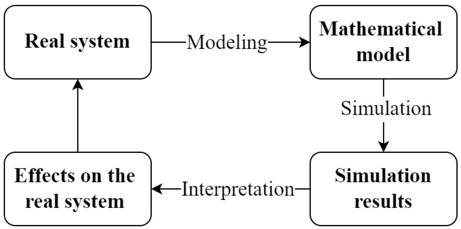
The most common approximation of a real system is achieved using mathematical models, developed through careful observation of its behavior and the impact that an estimated model can have on the real process (see Figure 1). In the literature on vehicle dynamics modeling, several approaches are identified: using models that reflect only a single dynamic, either longitudinal [22,23] or lateral [10,24]; combining two models to result in decoupled modeling [18,19]; or using models that describe a dynamic as comprehensively as possible [10,25,26,27]. In [23], a comprehensive vehicle longitudinal model is proposed that includes vehicle dynamics (influenced by tire forces, aerodynamic drag, rolling resistance, and gravity) and power train dynamics (including the engine, transmission, and wheel dynamics) to realistically simulate wheel behavior during braking and throttling. A four-wheel dynamic model is used, which is able to represent behavior that is similar to a real vehicle; it achieved good performance for high velocity values. Rajamani very explicitly described the bicycle model for the lateral dynamics in [10], which assumes the vehicle’s front and rear axles can be represented as single points. The key elements include the lateral forces acting on the tires, the yaw moment, and the resulting vehicle behavior, e.g., side-slip and yaw rate. One disadvantage of this model is the sensitivity in sudden driving conditions, such as sharp turns or high-speed maneuvers.

Figure 1.
Model estimation.
Models are divided into two categories: linear and nonlinear. Many studies have demonstrated the efficiency of linear models [28,29], which are frequently used due to their reduced complexity and exclusion of variable parameters. However, nonlinear models offer a closer representation of reality when it comes to vehicle dynamics [30].
2.2. Control Techniques
The design of control strategies that can handle system dynamics, especially during evasive maneuvers at high speed or emergency driving, has proven to be very efficient in the development and implementation of automated technologies. In terms of challenging driving situations, the main components that stand out are as follows: risk monitoring, driver monitoring, decision making, and path planning and control [31]. For such a controller, many works have proposed control strategies such as PID control [32], linear quadratic regulator (LQR) [33], or sliding mode control (SMC) [34]. The limitations of these methods are that they are not inherently optimal and are not well-suited for handling constrained optimization problems [31].
A suitable algorithm for vehicle control is MPC, which is an optimal control technique designed to predict future states of the model and can additionally handle nonlinearities. In [12], Camacho offers a detailed explanation and an ample study about the benefits and implementation of model predictive control. He demonstrates that MPC should not be seen only as a technique for managing linear and relatively slow processes.
The recent advancements have shown promising results in these areas, with emerging applications in nonlinear and hybrid processes. The dominance of linear models in MPC applications is due to their ease of identification from process data and effectiveness near specific operating points; this simplicity has significantly contributed to their commercial success.
The term nonlinear MPC (NMPC) refers to predictive controllers using nonlinear dynamic models, which introduce additional complexity. NMPC becomes essential in scenarios where process nonlinearities are significant, and market demands necessitate frequent operational changes.
The main advantages of MPC are its ability to manage a large number of variables and constraints [35], as well as its enhanced tracking performance at medium to high lateral and longitudinal accelerations [36]. Papers [37,38] provide relevant work in the field of integrating MPC into applications like controlling active front steering or differential brake for vehicle lateral stability. Control is essential for achieving automatic driving, with longitudinal control handling speed tracking and lateral control ensuring accurate steering [39].
2.2.1. Lateral Control
The goal of lateral control is to follow a trajectory, minimizing lateral and angular deviations to zero. It manages the vehicle’s yaw motion and the steering angle of the front wheels [39]. One of the most common studies on lateral control utilized a bicycle model [13], where a nonlinear MPC approach is proposed to solve the double-lane change maneuver. The controller proved to be efficient, but only for low velocity values. The works in [40,41] present results with a more accurate prediction of system dynamics, but with an increased computational load. In general, lateral control encompasses the concept of trajectory tracking, where the trajectory can either be a predefined path or computed online, this approach is also utilized in obstacle avoidance applications [42]. A comparative study of four path tracking controllers is presented in [42]. The analyzed methods include three classical algorithms—Pure Pursuit, Stanley controller, and Sliding Mode Control—along with a new kinematic lateral speed control. The fourth controller aims to enhance passenger comfort by smoothing lateral movements. The results analyze three criteria: precision at low speeds, stability, and passenger comfort. In terms of precision at low speeds, the proposed lateral velocity kinematic controller was the most accurate, with similar performance from the sliding kinematic controller. The kinematic controllers and Pure Pursuit provided the best comfort and safety, with smooth and precise movements. Regarding stability, all controllers except Stanley demonstrated good stability at all tested speeds.
2.2.2. Longitudinal Control
The controller for longitudinal dynamics is typically used in systems that manage the vehicle’s longitudinal motion. The study of longitudinal dynamics and control is found in many applications: adaptive cruise control, speed tracking, or velocity profile generation [18,19]. A solution to solve the ACC problem is proposed in [43], and represents a combination of motion planning and a hybrid MPC; the results proved to be satisfactory in terms of the tracking and computational calculation problem.
A solution using NMPC in a speed tracking application can be found in [44], where the controller uses an input integrator for improved robustness and speed, treating input derivatives as state variables. This method simplifies solving control equations, making the process faster and more efficient. A nonlinear control law for the longitudinal dynamics which also contains powertrain dynamics and gear ratio is proposed in [45]. The Lyapunov-based controller design ensures stability and convergence of the speed tracking error.
3. Vehicle Dynamics
Vehicles have multiple subsystems that interact under specific operating conditions. These interactions can significantly impact the effectiveness of decentralized control schemes that consider only local dynamics [25]. Therefore, a comprehensive vehicle model that includes relevant dynamic subsystems and their interactions is necessary.
Equations (1)–(3) present a model that integrates the body dynamics for longitudinal and lateral motion along with orientation [45]:
where m denotes the vehicle’s mass, the term represents the vehicle’s acceleration in the longitudinal direction x, while denotes the longitudinal velocity. Similarly, signifies the vehicle’s acceleration in the lateral direction y, while represents the lateral velocity. The term represents the angular acceleration, and denotes the yaw rate of the vehicle. The force is the longitudinal force applied to the vehicle and the term represents the resistant force opposing the motion, which includes aerodynamic drag and rolling resistance. The forces and represent the lateral forces acting on the front and rear tires, respectively. The distances a and b are the distances from the vehicle’s center of mass to the front and rear axles, respectively. This model accounts for various phenomena significantly influencing chassis dynamics, particularly in critical driving situations. It incorporates nonlinear longitudinal and lateral tire behavior, providing a robust framework for understanding and predicting the vehicle’s performance under complex conditions [25].
The vehicle coordinates in the fixed frame (X, Y, ) are calculated using the kinematic model given by [45]:
The forces used in Equations (4)–(6) are described as follows [10]:
where is the air density, A is the frontal area of the vehicle referring to the area of the vehicle that faces the airflow and contributes to the aerodynamic drag, represent the drag coefficient, and is the wind velocity.
The lateral forces contain the following parameters: and , which represent the cornering stiffness of the front and rear tires, respectively, and , which are the slip angles at the front and rear wheels, respectively, and , which is the steering angle.
The following relations can be used to calculate the slip angles [10]:
The lateral wheel velocities and the longitudinal wheel velocities are computed using [46]:
where the velocity components for each axis are described by [46]:
Assumption 1.
Steering is considered only for the front axle, with the steering angles of the front wheels assumed to be equal, i.e., , .
The presented complete model, given by Equations (1)–(6), represent the vehicle components in the proposed method for computing the maximum velocity profile and the trajectory tracking concept. This model serves as a mathematical representation of the dynamics of a real vehicle, capturing the essential aspects of its motion. It combines the longitudinal, lateral, and orientation dynamics, along with the forces applied and the velocities for each wheel. Note that this model is essential for advanced control strategies to optimize the vehicle’s performance and safety.
4. Velocity Profile
The generation of a maximum velocity profile for a vehicle involves determining the maximum speed that the vehicle can achieve under specific conditions. This aspect is essential for understanding the vehicle’s performance capabilities and is influenced by various factors, including road topography.
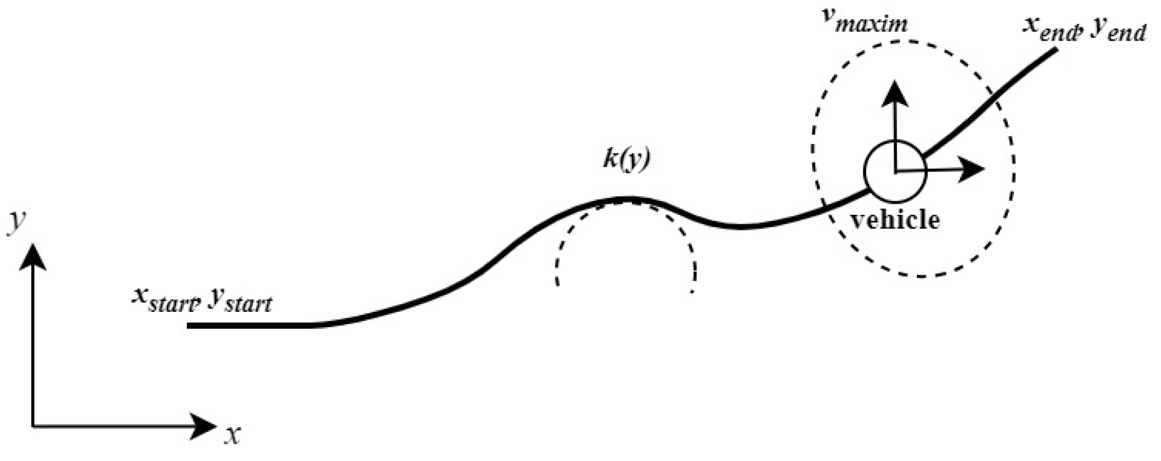
The presented concept (see Figure 2) involves the vehicle moving along a predefined road, with known maximum velocity limits, acceleration and deceleration parameters, and trajectory given in Cartesian coordinates. The path is described by its curvature , which indicates how sharply a curve bends at a particular point. The objective is to determine the optimal velocity profile that enables the vehicle to safely adhere to the specified trajectory with a minimum total travel time [47].
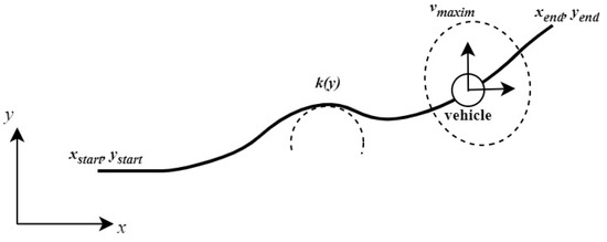
Figure 2.
Vehicle traveling along a given road with maximum velocity limit.
To describe the curvature of the trajectory, the following equation is used as follows:
The first step in obtaining the velocity profile for a vehicle along its trajectory is to compute the maximum velocity allowed for the vehicle at each point along its path [48]:
The forward integration step provides the integration of the acceleration parameter, i.e., , thereby enabling the vehicle to incrementally increase its velocity. The value obtained from Equation (22) is compared with that derived from Equation (21), and the minimum of the two values is selected [48] as follows:
The final step in the algorithm involves backward integration, during which the vehicle systematically reduces its velocity. This adjustment is made in response to the specific shape of the trajectory and is governed by the application of the deceleration parameter, i.e., , ensuring that the vehicle’s speed aligns accurately with the given path [48]:
In the final step of obtaining the velocity profile, the value calculated using Equation (23) is compared with the value from Equation (22). The minimum of these two values is selected to ensure the most appropriate velocity adjustment according to the system’s constraints and requirements.
To provide a comprehensive overview of the proposed algorithm, a logical diagram is illustrated in Figure 3. In this diagram, represents the velocity computed using (21), is derived from (22), and is calculated using (23). This visual representation aids in understanding the sequential application of these equations in the algorithm’s process flow.
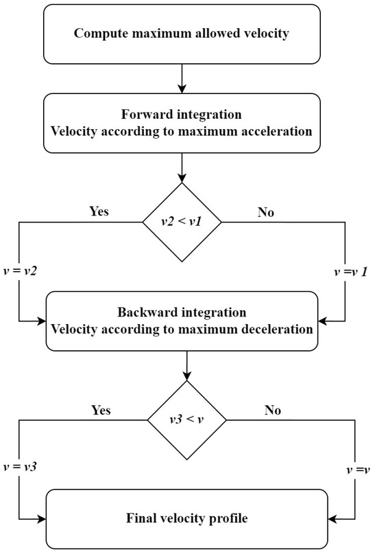
Figure 3.
Logical diagram for the velocity profile algorithm.
Furthermore, based on a fundamental assumption, it is considered that the velocity values are always greater than or equal to zero [47], thereby prohibiting any movement in the reverse direction. This constraint ensures that the velocity parameters adhere strictly to forward motion scenarios within the algorithm’s operational framework.
5. Nonlinear MPC Design
The foundation of model predictive control (MPC) lies in its ability to use a prediction model of the dynamic system. This model implies the computation of the future states of the system over a predetermined finite time horizon. By iteratively solving an optimization problem at each time step, MPC determines the optimal control actions while respecting system constraints. The optimization problem incorporates the system’s dynamics, predicted future states, control inputs, and constraints on states and inputs, ensuring that the control actions are both feasible and optimal over the specified prediction horizon.
The dynamic system can be described as a state-space model [45]:
where is the state-space representation of the vehicle model, u is the control input, is the sample time, and is the state-space vector.
The state-space vector and the control input are defined as follows:
The cost function to be minimized is formulated as follows:
with the following components:
where h and represent the predicted and the reference outputs, is the weighting matrix associated with the tracking error, and is the weighting matrix associated with the control input. These parameters determine the performance of the MPC feedback control [45]. The goal of this cost function is to minimize the sum of the squared differences between the predicted outputs and the reference outputs over the prediction horizon , as well as to minimize the control input effort.
The position of the vehicle is given by the global coordinates and the heading angle . These parameters, together with the longitudinal velocity , define the reference signal: .
Thus, the NMPC problem is formulated as follows [45]:
where is the discrete state-space representation of , U is the optimization vector, and and are the lower and upper limits of the control input u, respectively.
The state variable must range from zero to the maximum velocity determined by the velocity profile algorithm. To ensure this condition is met, the following constraints are imposed:
Following the implementation of the nonlinear model predictive control algorithm, we address the trajectory tracking problem by minimizing the difference between the reference trajectory and the obtained trajectory. Simultaneously, one can employ the velocity profile algorithm to ensure the vehicle moves safely along the path. This dual approach enables precise trajectory tracking and enhances the safety and stability of the vehicle’s motion.
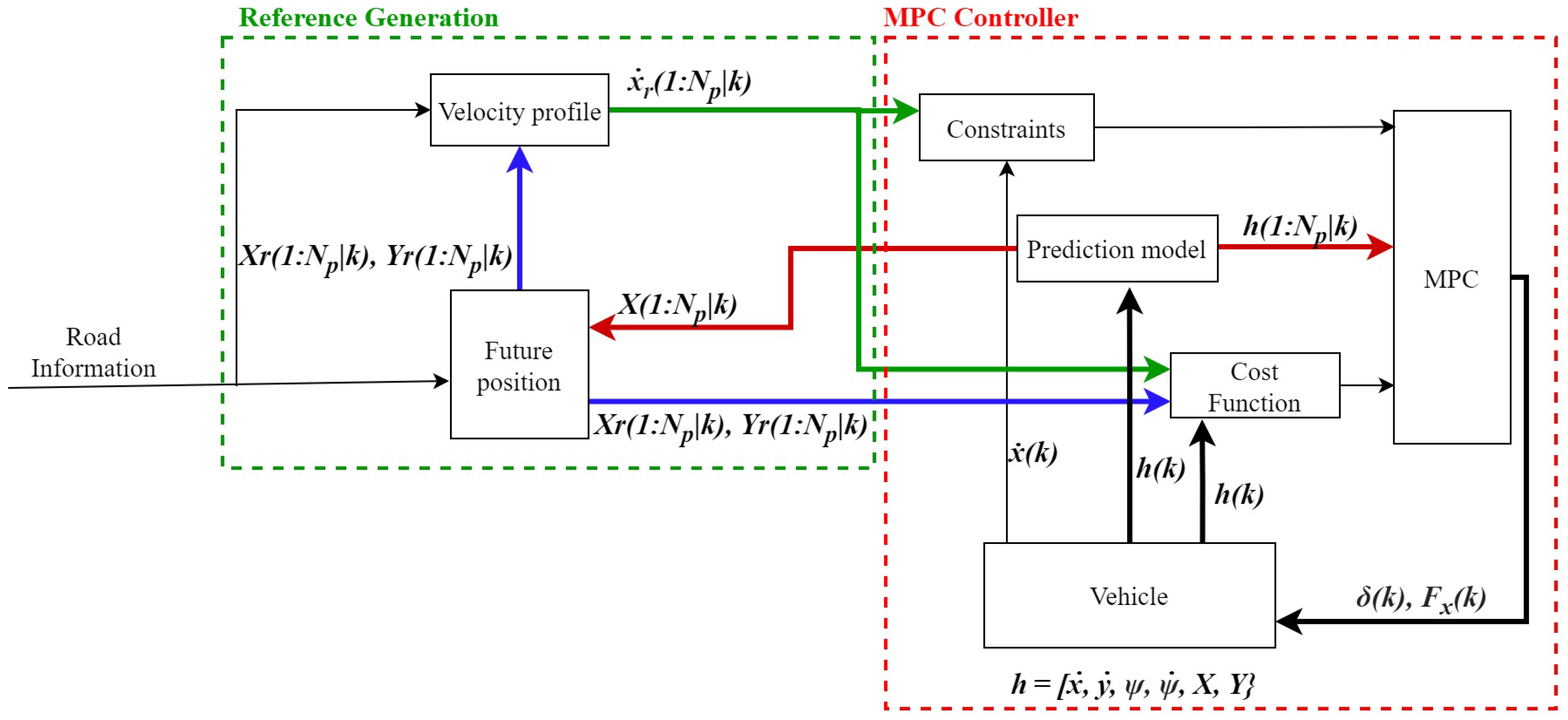
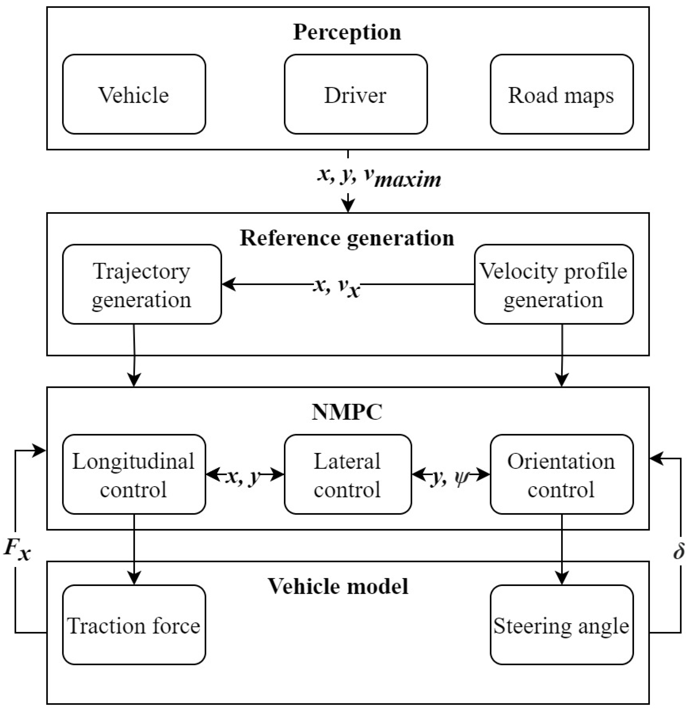
The diagram shown in Figure 4 illustrates the advanced control framework for vehicle dynamics described in this paper, utilizing model predictive control. The process initiates with the collection of road data, which are used to generate future reference positions for the vehicle over the prediction horizon, represented as and for each current time step k. Additionally, a velocity profile is created to outline the desired speeds over the prediction horizon. With these reference trajectories and velocities established, the MPC controller calculates the optimal control actions. The embedded prediction model within the MPC uses the vehicle’s current state to forecast the future states over the prediction horizon. Concurrently, the controller evaluates a cost function that quantifies how closely the predicted states match the reference trajectories and velocities. This cost function also accounts for the required control efforts by penalizing deviations from the reference trajectories. Additionally, it considers the values of reference inputs related to lateral velocity and yaw rate , assuming them to be zero to ensure smooth and efficient driving behavior. The motivation for including these terms is to maintain stability and improve the overall driving experience. Constraints are enforced to ensure that the predicted velocity stays within safe and feasible limits. The MPC algorithm then optimizes the control inputs, specifically the steering angle and the longitudinal force . These optimized control inputs are applied to the vehicle, which updates its state accordingly. The updated vehicle state is then fed back into the system, facilitating continuous real-time adjustments.
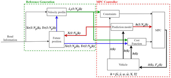
Figure 4.
Control architecture for vehicle dynamics.
This feedback loop ensures that the vehicle consistently follows the reference trajectory while adhering to dynamic constraints and minimizing control efforts. By continuously predicting future states, evaluating costs, and optimizing control actions in real time, the MPC framework effectively governs the vehicle’s path, thereby enhancing both safety and performance on the road.
6. Road Extraction
The road used to obtain the simulation results is extracted from online mapping platforms. The conventional method for defining a roadway in applications that utilize the Global Positioning System (GPS) is through the use of geographical coordinates, specifically latitude and longitude.
The dynamic model for the vehicle, along with the algorithms for control and velocity profiling, utilize Cartesian coordinates. Consequently, it is necessary to convert the latitude and longitude coordinates to Cartesian coordinates, as described in (34) and (35):
where R is the radius of the Earth in meters, defines the selected value for longitude, and represents the selected value for latitude. The component defines the functions which are used to convert the latitude to a corresponding value for the lateral coordinate y in the Cartesian system:
This transformation is commonly used in cartography and map projections to handle the distortion that occurs at higher latitudes.
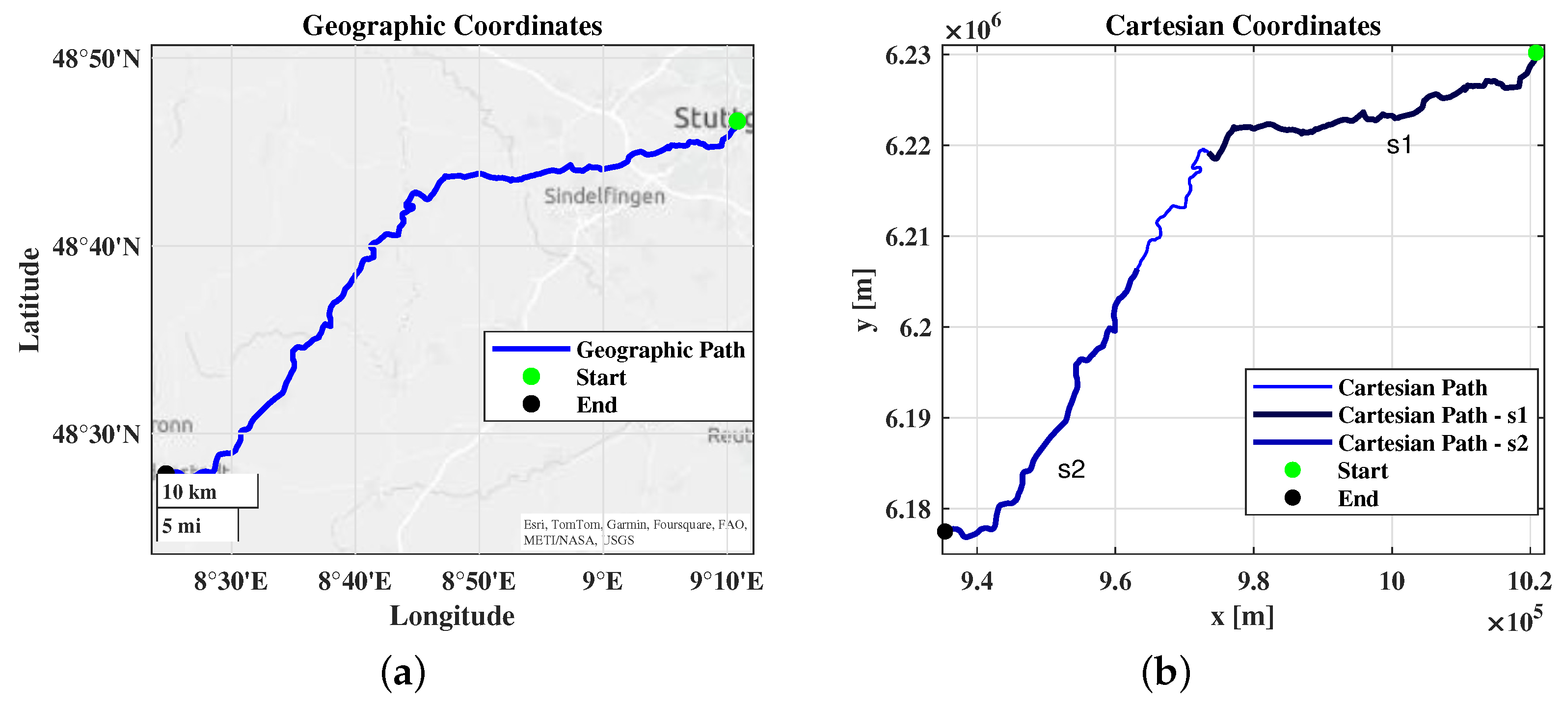
In Figure 5a, the selected route (70,173 Stuttgart to 72,250 Freudenstadt, Germany) from the online mapping platform is depicted using geographical coordinates. The starting point is indicated at (48.7773° N, 9.1803° E) and the ending point is at (48.4640° N, 8.4119° E). Additionally, the corresponding Cartesian coordinates (see Figure 5b) resulting from the conversion algorithm confirm the desired approach, which can be effectively utilized in the proposed implementation.
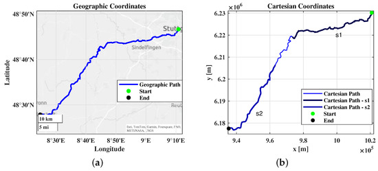
Figure 5.
Conversion from geographical coordinates to Cartesian coordinates: (a) trajectory described in geographical coordinates, (b) trajectory described in Cartesian coordinates.
The road in Figure 5a is divided into two segments: and . This segmentation will result in shorter trajectories, simplifying the analysis of the obtained trajectory data. To ensure a realistic implementation, it is necessary to determine the maximum legal speed for each road segment within the entire obtained trajectory. This will allow the results to be compared accurately with real-world data and the information from various mapping platforms.
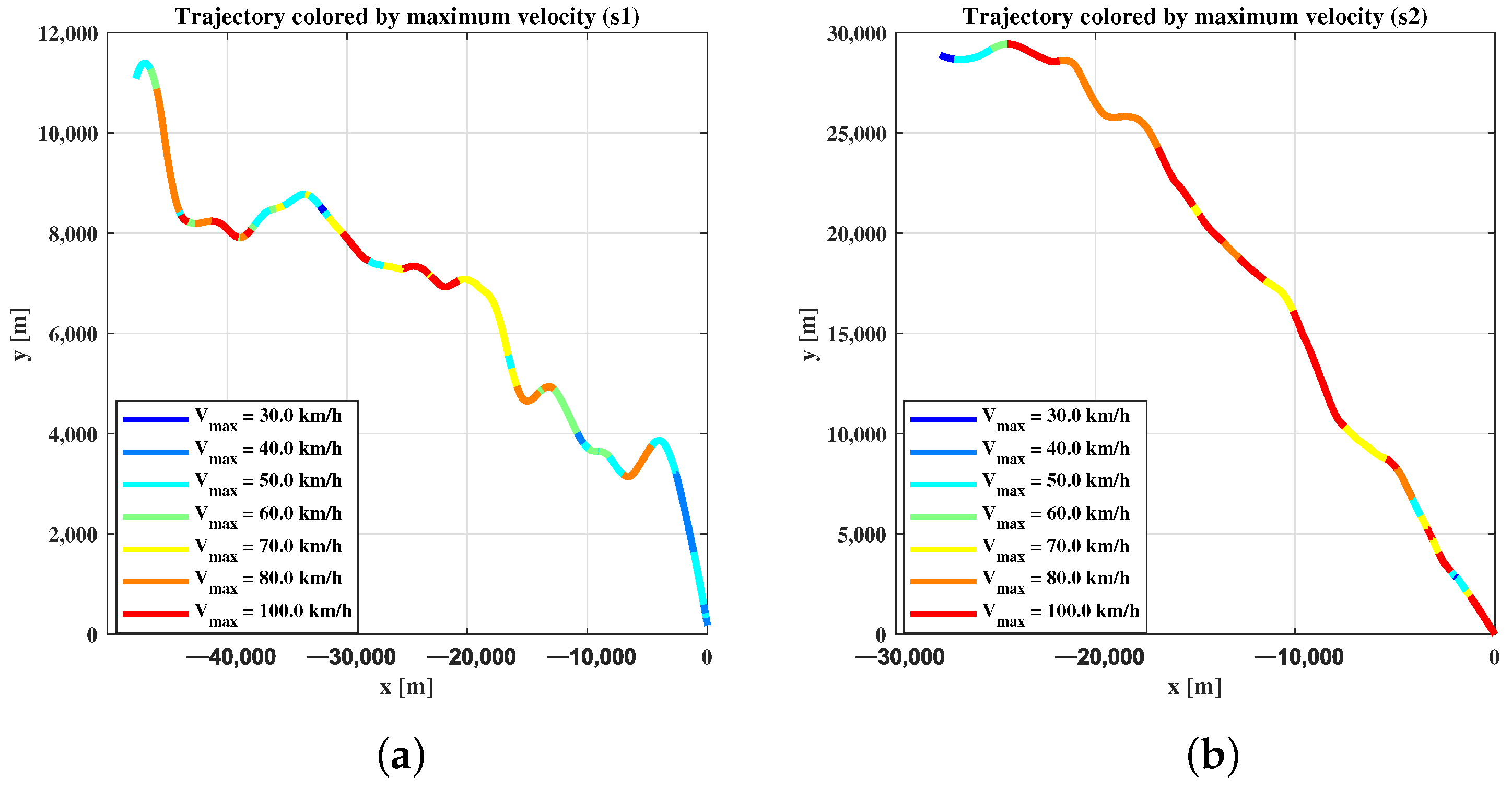
Moreover, the first road segment, , features a path where the maximum velocity limits are lower compared to the second segment, , which predominantly has higher speed limits (see Figure 6 as an illustration).
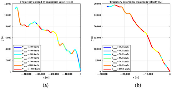
Figure 6.
Colored trajectory according to legal maximum velocity limits: (a) first road segment s1, (b) second road segment s2.
In Figure 6, the trajectory is presented, color-coded according to the maximum velocity limits for each segment. The trajectory has been translated to zero to facilitate clarity and enhance computational efficiency.
The motivation for selecting this road is supported by the numerous velocity segments and the curves that constitute the road. These aspects increase the difficulty of following the road and will demonstrate the efficiency of the proposed approach for the velocity profile and trajectory tracking algorithm.
The selected trajectory is composed of a series of points with a distance of approximately one meter between each of them. For this reason, it cannot be passed through each point precisely due to the vehicle’s higher velocity. To navigate the entire route at the maximum allowed velocity, the following logic, as described in Algorithm 1, is implemented.
| Algorithm 1 Trajectory Following and Velocity Profile Algorithm |
|
The reference states are initialized with the first elements, where represents the prediction horizon. The reference velocity is computed using the algorithm specified by Equations (20)–(23). Subsequently, applying the control method to the dynamic system allows for the prediction of future states of the process, including the future position described by coordinates (). Given the predicted future position, determined based on the vehicle’s velocity, the estimated point on the trajectory that the vehicle will achieve can be computed. Finally, the future reference is updated according to this prediction, and the entire process is iteratively repeated until the vehicle reaches the end point of the trajectory.
7. Illustrative Results
This section presents the results obtained by applying the proposed control method to the dynamic system. Additionally, it includes the implementation details and performance outcomes of the velocity profile algorithm. Note that a preliminary processing of the trajectory data was performed to enhance its suitability for further analysis.
For the NMPC simulation, MATLAB software was utilized, and the optimization problem was solved using the fmincon solver due to its capability to handle nonlinear objective functions and constraints. It offers flexible constraint management, accommodating both equality and inequality constraints, which are essential for maintaining system safety and performance limits. The solver employs gradient-based optimization methods, enhancing efficiency, particularly when gradients are provided or computed.
Figure 7 illustrates the structured implementation within the proposed application, providing a clearer understanding of the connectivity between the algorithms discussed in the previous sections. The description of each step of the implementation is provided as follows:
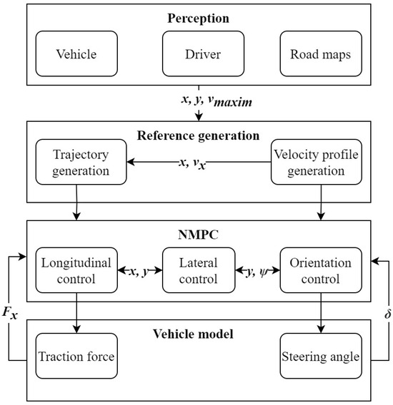
Figure 7.
Implementation Architecture of the Application Framework.
- Perception: This provides information describing the trajectory coordinates () and maximum allowed velocity values for each road segment.
- NMPC: In this module, the reference for the vehicle states is received. By applying the nonlinear model predictive control (NMPC) algorithm, the control signals, including traction force and steering angle, are computed.
- Vehicle model: Iteratively, at each time step, the future states of the dynamic process are estimated and computed based on the results obtained from the controller.
The vehicle model used in this study is described by Equations (1)–(19), where the vehicle state variables are shown in Table 1 and the constant parameters are shown in Table 2.

Table 1.
Vehicle State Variables.
Table 2.
Vehicle Constant Parameters.
To accord the controller, we use the sample time seconds and the following tuning parameters:
The selection of NMPC parameters is essential for achieving optimal performance. For the proposed application, parameters are chosen based on a combination of theoretical guidelines and empirical tuning.
The velocity constraints for each time step are defined such that the velocity must lie within the range , where represents the reference velocity, as is expressed in (33). In this manner, we ensure that the velocity does not exceed the reference value calculated by the planner. In our case, the maximum allowable speed is 100 km/h.
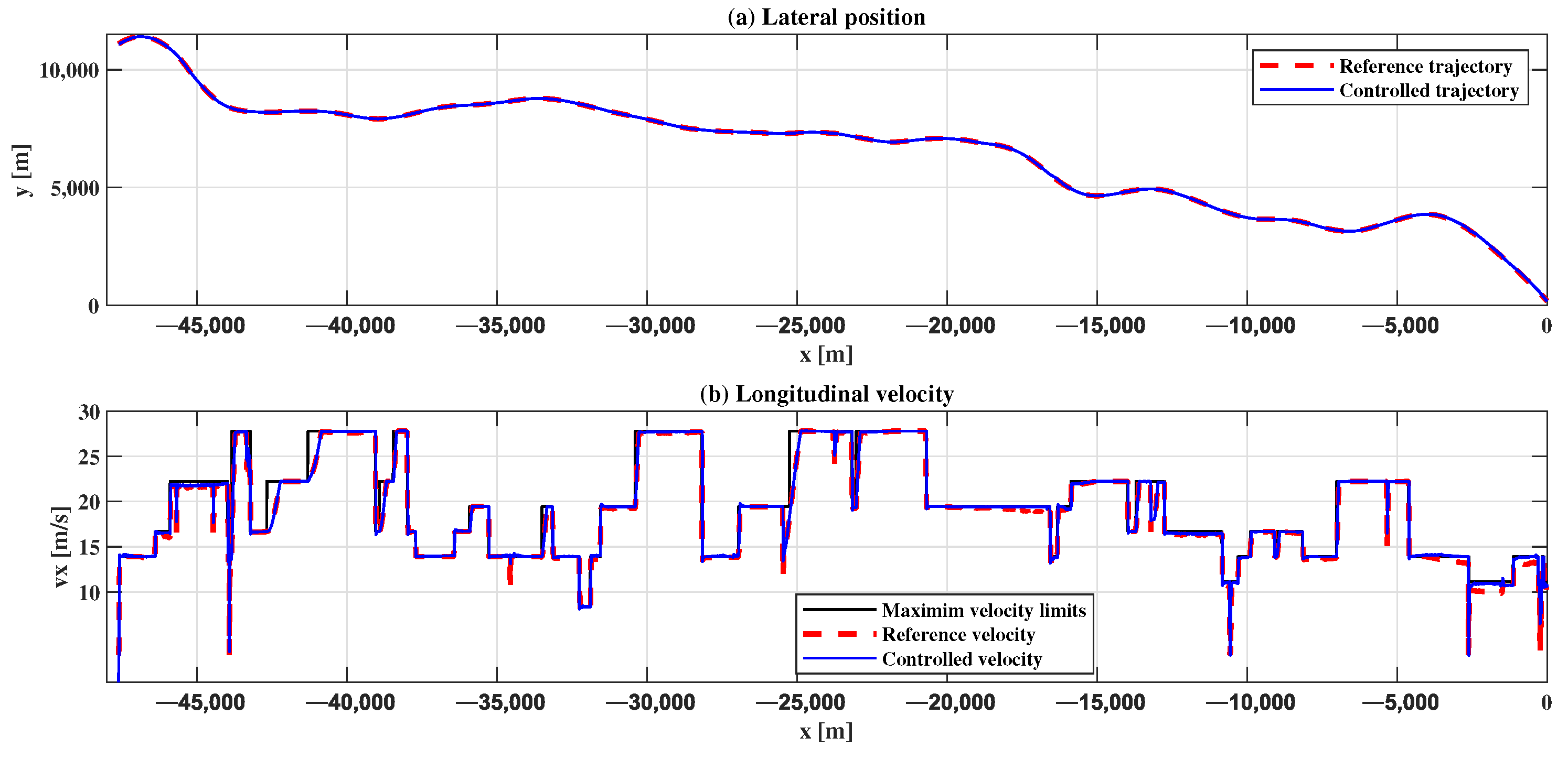
7.1. First Road Segment—s1
For the first proposed scenario represented by the road segment , Figure 8 illustrates the results obtained with the proposed control method used for both the lateral and longitudinal dynamics.
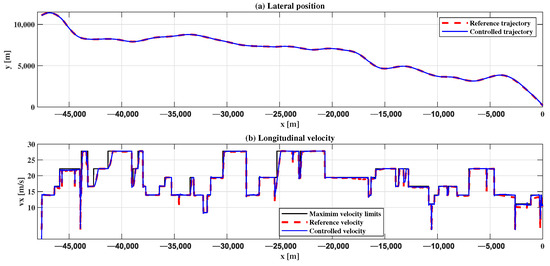
Figure 8.
First road segment—s1: (a) trajectory tracking, (b) velocity profile.
The longitudinal dynamic is represented by the longitudinal velocity, which is obtained using the velocity profile algorithm described by Equations (20)–(23).
As illustrated, the key points of the proposed algorithm are achieved; the maximum velocity computed does not exceed the legally imposed speed limit. Moreover, the transition between a lower limit to a higher one is not instantaneous, but instead follows a ramp response, which is physically accurate and represents a natural behavior for velocity. Additionally, when a curved trajectory is followed, the algorithm decreases the velocity to ensure safe movement along the road.
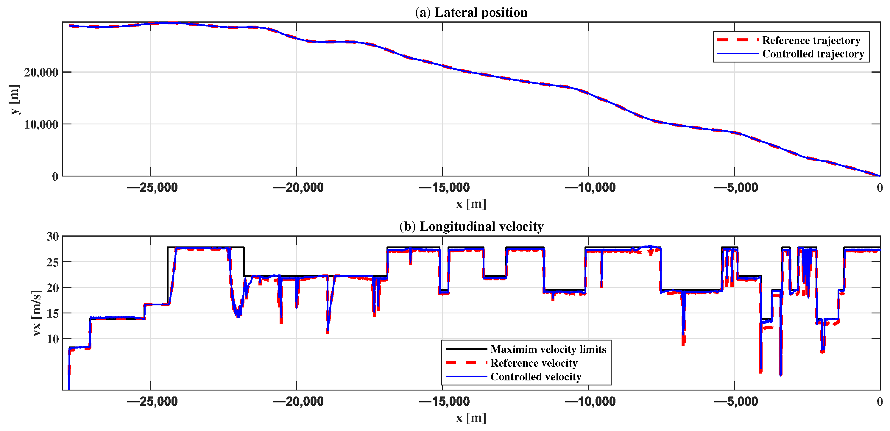
7.2. Second Road Segment—s2
In the second proposed scenario illustrated in Figure 9, the difference is characterized by the higher maximum velocity limits imposed. This aspect increases the complexity and difficulty of the velocity adaptation algorithm, especially during tight maneuvers where the vehicle needs to decrease its velocity to ensure good trajectory following.
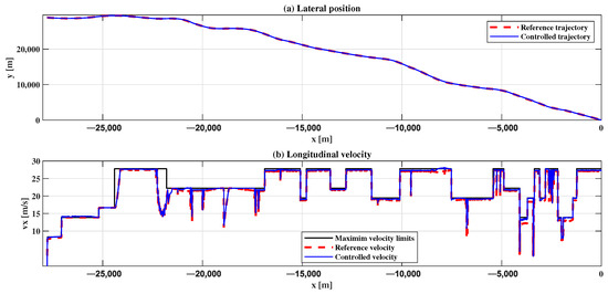
Figure 9.
Second road segment—s2: (a) trajectory tracking, (b) velocity profile.
The top graph in Figure 9 shows the lateral position, in which one can observe the close alignment between the reference and the controlled trajectory that demonstrates the effectiveness of the controller in maintaining the correct position with minimal deviation. The velocity is illustrated in the bottom graph, and the obtained results indicate the effectiveness of the velocity profile algorithm. Similarly to the first scenario, the maximum legal velocity is respected, and the speed is correctly adapted to account for road curvature, ensuring accurate trajectory following. The controller effectively reduces the velocity where necessary to maintain safe and smooth navigation along the trajectory.
8. Performance Analysis and Discussion
For a comprehensive analysis, in addition to the graphical representation, performance values for both road segments, and , were computed. This numerical analysis will allow us to better observe the influence of higher velocity values on the performance metrics.
8.1. Performance Metrics
The performance metrics represent an efficient method to evaluate obtained results, each offering unique insights into model accuracy and error characteristics. These metrics provide an interpretation of the average prediction error and a comprehensive measure of overall error magnitude, facilitating optimization.
8.1.1. Mean Squared Error (MSE)
The mean squared error (MSE) is calculated as the average of the squares of the differences between the predicted and actual values [49]:
8.1.2. Root Mean Squared Error (RMSE)
The root mean squared error (RMSE) provides an error measure in the same unit as the target variable [49]:
8.1.3. Mean Absolute Error (MAE)
The mean absolute error (MAE) is calculated as the average of the absolute differences between the reference and controlled velocities [50]:
8.1.4. Correlation Coefficient
The Correlation Coefficient (often denoted as r) measures the linear relationship between the reference and controlled velocities [49]:
where is the reference velocity, is the controlled velocity, is the mean of the reference velocities, is the mean of the controlled velocities, and n is the number of observations.
8.1.5. Distribution and Cumulative Distribution Function
To interpret the obtained results, the usage of the distribution and cumulative distribution function (CDF) analysis provides a deep understanding of the system’s dynamics, enabling the design of effective and resilient control solutions. These also represent essential tools in the following:
- Understanding and characterizing system behavior;
- Evaluating and improving control performance;
- Supporting predictive control strategies.
8.2. Numerical Results for the Longitudinal Dynamics
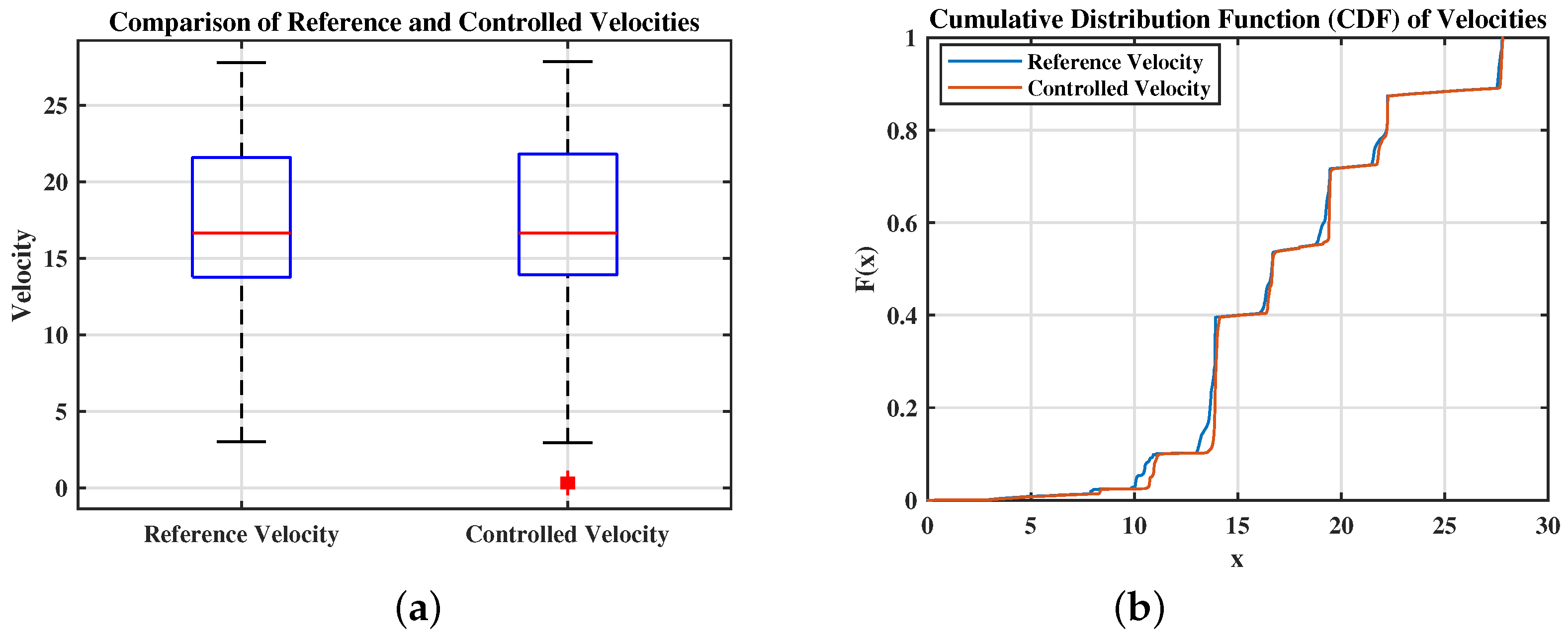
The distribution and CDF analysis for the first road segment, , are illustrated in Figure 10. In the case of the distribution results, one can observe that the medians and interquartile ranges (IQRs) of the reference and controlled velocities are very similar, indicating that the controlled velocities closely follow the reference velocities in terms of central tendency and variability. The cumulative distribution function (CDF) results indicate that the distribution of the controlled velocities closely matches that of the reference velocities across all three categories of values: low, mid, and high. There are some very minor deviations, but these have a minimal impact on the overall system performance.
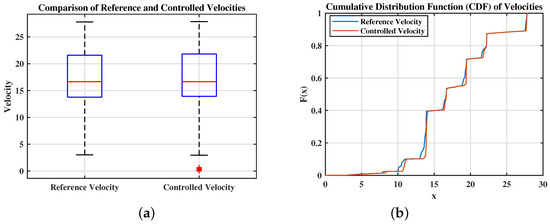
Figure 10.
Performance analysis for s1: (a) distribution of velocity, (b) cumulative distribution function of velocity.
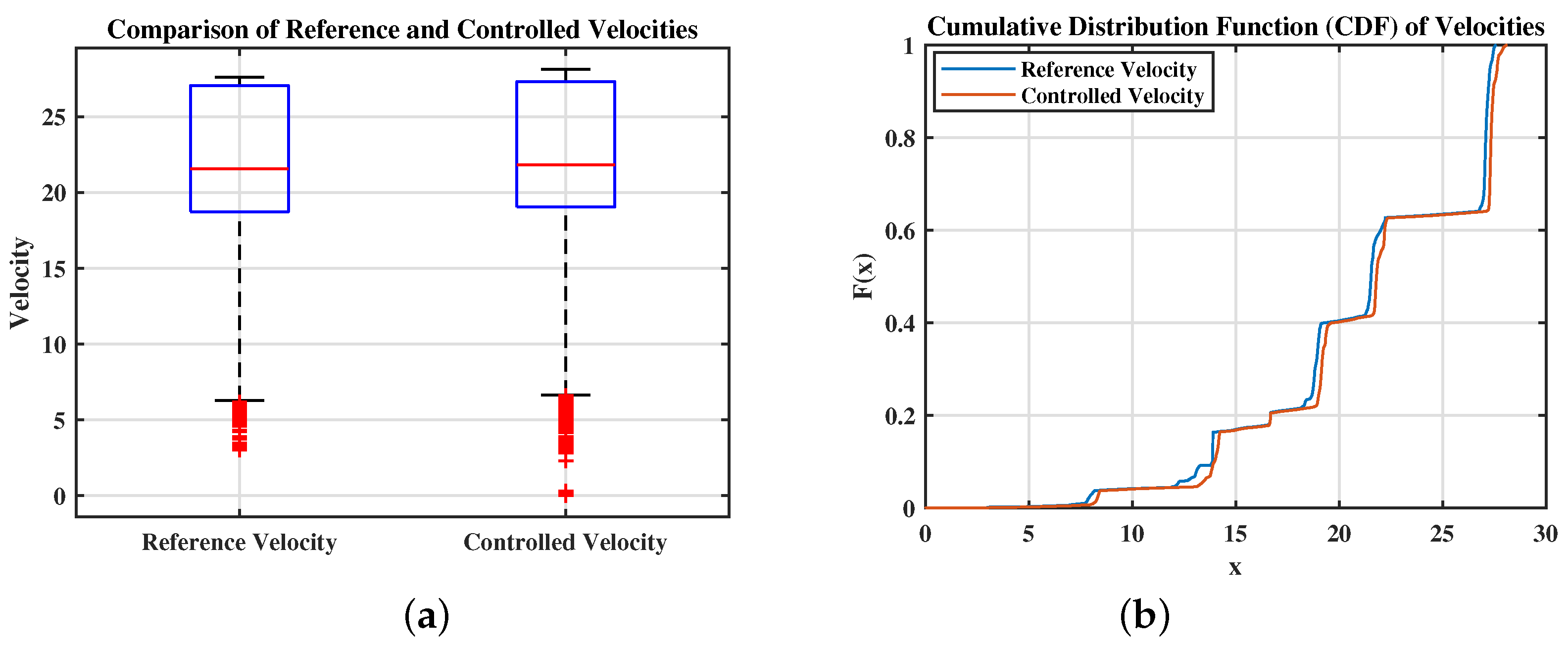
For the second proposed scenario, , the results obtained regarding the distribution show many outliers below the lower whisker, as can be seen in Figure 11. This behavior is expected, considering the difficulty the vehicle faces when it needs to decrease its velocity rapidly from a high value to a low one in order to stay on the road during tight curves. Here, the influence of high velocity values on the vehicle can be better observed, demonstrating how they increase the difficulty in maintaining control and trajectory following. However, the similar overall ranges admit that the controlled velocity follows the reference one. In the case of the CDF curves for both datasets, they are very close, indicating a matched distribution.
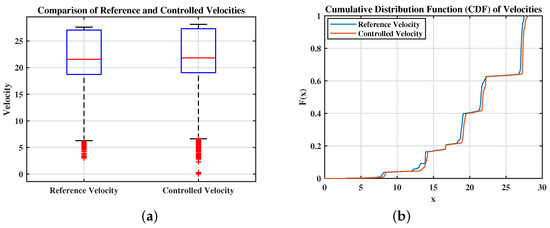
Figure 11.
Performance analysis for s2: (a) distribution of velocity, (b) cumulative distribution function of velocity.
In Table 3, the numerical results of the error-based performance metrics and the correlation coefficient calculated using Equations (37)–(40) are presented. The low values for the performance metrics indicate good control performance, and the value obtained for the correlation coefficient, which is almost equal to 1, represents an almost perfect linear relationship for both proposed scenarios.
Table 3.
Velocity Performance Metrics.
8.3. Numerical Results for the Lateral Dynamics
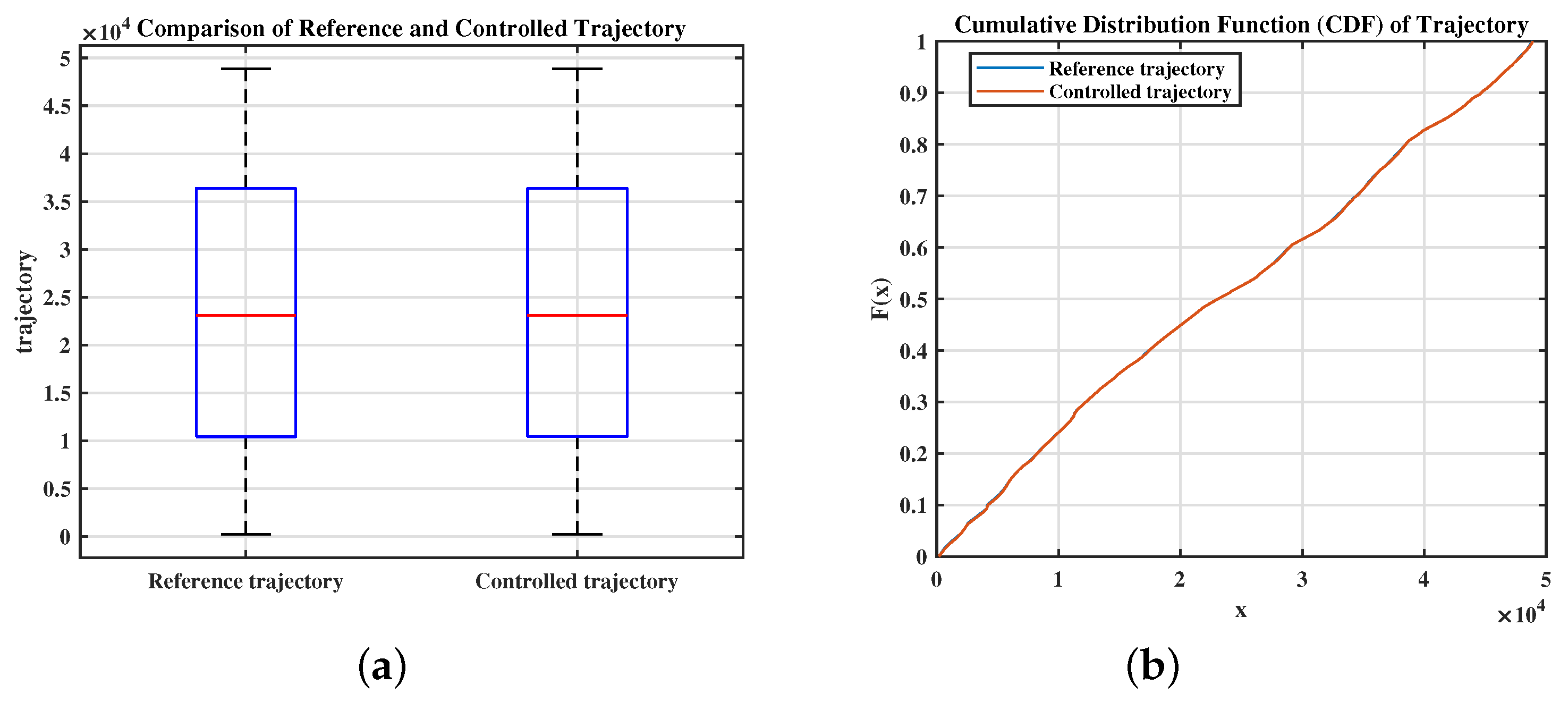
Regarding the analysis of the performance metrics for the trajectory in the first case, i.e., , the results of the distribution and the cumulative distribution function are illustrated in Figure 12. Analyzing the figures on the left and the right, one can observe that the controlled trajectory follows the reference trajectory, highlighting the similarities between the median and the spread. Additionally, it shows an alignment of the distributions.
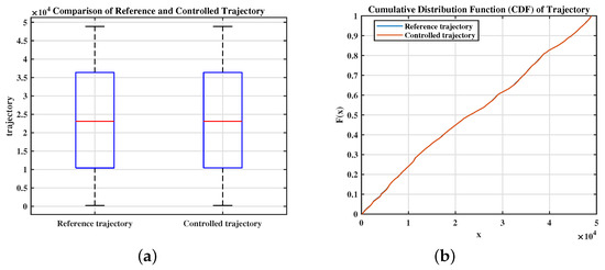
Figure 12.
Performance analysis for s1: (a) distribution of trajectory, (b) cumulative distribution function of trajectory.
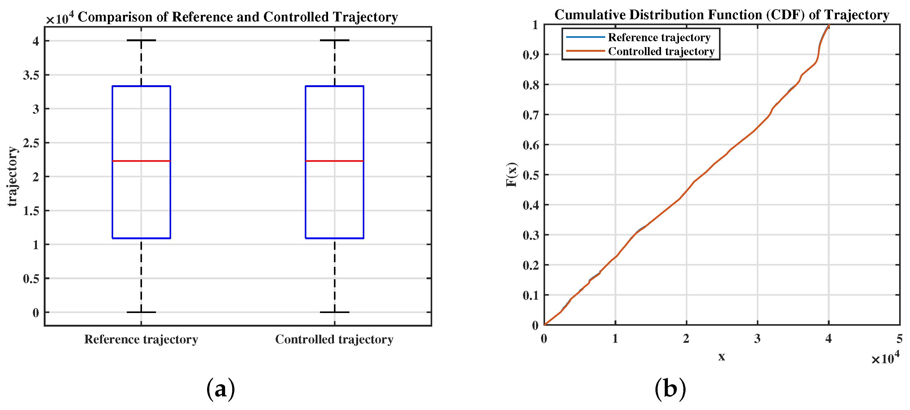
For the second case, i.e., , the results illustrated in Figure 13 confirm the efficiency of the controller once again, with the controlled trajectory closely following the reference trajectory.
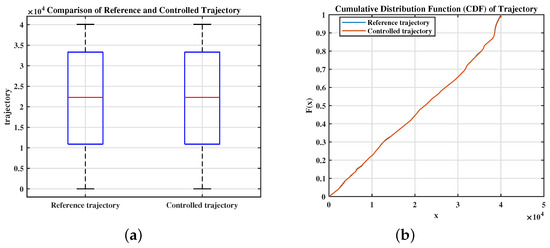
Figure 13.
Performance analysis for s2: (a) distribution of trajectory, (b) cumulative distribution function of trajectory.
Table 4 shows the values of the performance metrics for the two cases. The small values of the errors demonstrate the controller’s good accuracy with a minimum magnitude of the errors, and the correlation coefficient, in both cases, indicates a perfect linear relationship between the two trajectories.
Table 4.
Trajectory Performance Metrics.
Considering all the results presented for the proposed scenarios, both graphical and numerical, we can conclude that the controlled velocities closely follow the reference velocities. This indicates good control performance, allowing the vehicle to move smoothly and safely along the given trajectory.
8.4. Discussion
The proposed application, as demonstrated by the results, achieves satisfactory performance in guiding a vehicle along a specified route. It ensures safety while allowing the vehicle to reach its maximum speed, all within the legal limits imposed.
The main contribution of this paper is the development of a framework that uses a nonlinear model to describe vehicle dynamics. This type of model brings the framework closer to the real behavior specific to a vehicle. To handle the nonlinearities, an NMPC (nonlinear model predictive control) controller is used, with constraints imposed on the velocity. Furthermore, this paper introduces a new perspective by using a real road as a reference trajectory, obtained from online mapping platforms. Most existing studies typically address trajectory issues through simpler scenarios, such as lane changes [51] or trajectories generated using methods like quartic function [52] or spline interpolation [53].
A realistic approach to road dynamics can be found in studies examining the behavior of racing cars on renowned circuits such as Silverstone [54] or Thunderhill Raceway [55]. The findings from these studies validate the effectiveness of various control methods; however, they primarily focus on vehicles operating in high-speed, aggressive driving conditions. In the method proposed in this paper, we analyze a standard route that reflects typical driving scenarios. Furthermore, we adopt a more realistic perspective on vehicle speed. To achieve this, we impose legal speed limits based on the selected routes, ensuring that the vehicle adheres to these constraints. Additionally, the integrated velocity algorithm effectively captures a range of driving behaviors, allowing for speed adaptations that correspond to the road’s geometric characteristics. Due to the variability in speed values, it was essential to implement a strategy for generating trajectory points. This ensures that the proposed algorithm considers the vehicle’s velocity when estimating its future position. Based on this estimation, the algorithm selects a position point that is closer to the predicted trajectory.
The obtained research results can be applied to various automated vehicle applications. For instance, they can be used to estimate a more realistic driving time for a vehicle on a specific road. This estimation has advantages over existing online applications because it considers the time required for a vehicle to reach a new maximum velocity when transitioning from a road segment with a lower speed limit to one with a higher limit. Additionally, it accounts for situations where the trajectory includes tight curves that necessitate deceleration below the maximum legal speed, which also increases travel time. We propose future work to cover and develop more applications starting with the proposed framework.
Another key point to address is the portability of the proposed automated control system to different vehicles. The control algorithm can be tuned for different vehicle dynamics by adjusting the parameters within the NMPC. However, successful implementation on different vehicles would require thorough validation and calibration for each specific vehicle type to ensure optimal performance and safety.
Future research will focus on developing a more sophisticated vehicle model and integrating communication protocols to enable vehicle-to-vehicle (V2V) and vehicle-to-infrastructure (V2I) interactions. This will facilitate the creation of vehicle platoons that share environmental information, such as sensor data and road surface characteristics, leading to more realistic simulations. Additionally, we aim to implement an adaptive nonlinear model predictive control (NMPC) system capable of adjusting parameters in real time based on the vehicle’s current state and environment. Furthermore, the trajectory planning component will be enhanced to effectively manage unexpected obstacles and changes on the road.
9. Conclusions
In this paper, a framework is proposed that consists of a nonlinear model for vehicle dynamics controlled using a NMPC algorithm. This framework enables the implementation of a method for the maximum velocity profile and a trajectory tracking method. The vehicle dynamics are described by a nonlinear model that captures the longitudinal and lateral dynamics, as well as the orientation. The motivation for choosing this model lies in its ability to realistically simulate real-world behavior due to its complexity. It is important to note that the chosen trajectory plays a significant role in this context. To apply and test the algorithm, a road was extracted using online mapping platforms, and the maximum allowed velocities for each sector were identified. This approach enabled us to observe velocity behavior and highlight variations as the vehicle transitions between road segments with different speed limits. For the control part, a nonlinear model predictive control algorithm was implemented, an advanced method capable of handling nonlinearities effectively. Overall, the key points of this paper were achieved as follows: the results indicate good controller performance and the efficiency of the vehicle profile algorithm as the vehicle successfully manages to follow the imposed trajectory.
Author Contributions
Conceptualization, G.-S.P. and C.-F.C.; methodology, G.-S.P. and C.-F.C.; software, G.-S.P.; validation, G.-S.P. and C.-F.C.; formal analysis, G.-S.P. and C.-F.C.; investigation, G.-S.P. and C.-F.C.; resources, G.-S.P. and C.-F.C.; data curation, G.-S.P.; writing—original draft preparation, G.-S.P.; writing—review and editing, G.-S.P. and C.-F.C.; visualization, G.-S.P.; supervision, C.-F.C. All authors have read and agreed to the published version of the manuscript.
Funding
This research received no external funding.
Data Availability Statement
Data is contained within the article.
Conflicts of Interest
The authors declare no conflicts of interest.
Abbreviations
The following abbreviations are used in this manuscript:
| MPC | Model Predictive Control |
| NMPC | Nonlinear Model Predictive Control |
| ACC | Adaptive Cruise Control |
| MSE | Mean Squared Error |
| RMSE | Root Mean Squared Error |
| MAE | Mean Absolute Error |
| CDF | Cumulative Distribution Function |
| V2V | Vehicle-to-Vehicle Communication |
| V2I | Vehicle-to-Infrastructure Communication |
References
- Claussmann, L.; Revilloud, M.; Gruyer, D.; Glaser, S. A Review of Motion Planning for Highway Autonomous Driving. IEEE Trans. Intell. Transp. Syst. 2019, 21, 1826–1848. [Google Scholar] [CrossRef]
- Song, X.; Gao, H.; Ding, T.; Gu, Y.; Liu, J.; Tian, K. A Review of the Motion Planning and Control Methods for Automated Vehicles. Sensors 2023, 23, 6140. [Google Scholar] [CrossRef] [PubMed]
- Selby, M. Intelligent Vehicle Motion Control. Ph.D. Thesis, University of Leeds, Leeds, UK, 2003. [Google Scholar]
- Meng, Y.; Ming, W.; Gu, Q.; Liu, L. A Decoupled Trajectory Planning Framework Based on the Integration of Lattice Searching and Convex Optimization. IEEE Access 2019, 7, 130530–130551. [Google Scholar] [CrossRef]
- Reda, M.; Onsy, A.; Haikal, A.Y.; Ghanbari, A. Path planning algorithms in the autonomous driving system: A comprehensive review. Robot. Auton. Syst. 2024, 174, 104630. [Google Scholar] [CrossRef]
- Subosits, J.; Gerdes, J. From the Racetrack to the Road: Real-Time Trajectory Replanning for Autonomous Driving. IEEE Trans. Intell. Veh. 2019, 4, 309–320. [Google Scholar] [CrossRef]
- Svensson, L.; Bujarbaruah, M.; Kapania, N.; Törngren, M. Adaptive Trajectory Planning and Optimization at Limits of Handling. In Proceedings of the IEEE/RSJ International Conference on Intelligent Robots and Systems (IROS), Macau, China, 3–8 November 2019. [Google Scholar]
- Carvalho, A.; Gao, Y.; Gray, A.; Tseng, E.; Borrelli, F. Predictive control of an autonomous ground vehicle using an iterative linearization approach. In Proceedings of the 16th International IEEE Conference on Intelligent Transportation Systems (ITSC 2013), The Hague, The Netherlands, 6–9 October 2013; pp. 2335–2340. [Google Scholar]
- Betz, J.; Wischnewski, A.; Heilmeier, A.; Nobis, F.; Stahl, T.; Hermansdorfer, L.; Lohmann, B.; Lienkamp, M. What can we learn from autonomous level-5 motorsport? In 9th International Munich Chassis Symposium; Springer: Berlin/Heidelberg, Germany, 2019; pp. 123–146. [Google Scholar]
- Rajamani, R. Vehicle Dynamics and Control; Springer Science & Business Media: Berlin/Heidelberg, Germany, 2006. [Google Scholar]
- Gray, A.; Ali, M.; Gao, Y.; Hedrick, J.; Borrelli, F. Integrated threat assessment and control design for roadway departure avoidance. In Proceedings of the 2012 15th International IEEE Conference on Intelligent Transportation Systems, Anchorage, AK, USA, 16–19 September 2012; pp. 1714–1719. [Google Scholar]
- Camacho, E.F.; Bordons, C. Model Predictive Control; Springer: Berlin/Heidelberg, Germany, 2004. [Google Scholar]
- Falcone, P.; Borrelli, F.; Asgari, J.; Tseng, H.E.; Hrovat, D. Predictive Active Steering Control for Autonomous Vehicle Systems. IEEE Trans. Control Syst. Technol. 2007, 15, 566–580. [Google Scholar] [CrossRef]
- Anderson, S.; Peters, S.; Pilutti, T.; Iagnemma, K. An Optimal-Control-Based Framework for Trajectory Planning, Threat Assessment, and Semi-Autonomous Control of Passenger Vehicles in Hazard Avoidance Scenarios. Int. J. Veh. Auton. Syst. 2010, 8, 190–216. [Google Scholar] [CrossRef]
- Gray, A.; Gao, Y.; Lin, T.; Hedrick, J.; Tseng, E.; Borrelli, F. Predictive control for agile semi-autonomous ground vehicles using motion primitives. In Proceedings of the 2012 American Control Conference (ACC), Montreal, QC, Canada, 27–29 June 2012; pp. 4239–4244. [Google Scholar]
- Liniger, A.; Domahidi, A.; Morari, M. Optimization-Based Autonomous Racing of 1:43 Scale RC Cars. Optim. Control Appl. Methods 2015, 36, 628–647. [Google Scholar] [CrossRef]
- Alrifaee, B.; Maczijewski, J. Real-time Trajectory optimization for Autonomous Vehicle Racing using Sequential Linearization. In Proceedings of the 2018 IEEE Intelligent Vehicles Symposium (IV), Changshu, China, 26–30 June 2018; pp. 476–483. [Google Scholar]
- Pauca, G.S.; Caruntu, C.F. Automated Computing and Tracking of the Maximum Velocity on a Certain Road Sector. In Proceedings of the 26th International Conference on System Theory, Control and Computing, Sinaia, Romania, 19–21 October 2022; pp. 588–593. [Google Scholar]
- Pauca, G.S.; Caruntu, C.F. Velocity Computation for Vehicle Trajectory Tracking: A Comparative Analysis of Performance and Efficiency. In Proceedings of the 2023 24th International Conference on Control Systems and Computer Science, Bucharest, Romania, 24–26 May 2023; pp. 41–47. [Google Scholar]
- Pauca, G.S.; Caruntu, C.F. Trajectory Extraction from Online Mapping Platforms: Empowering Vehicle Dynamics and Intelligent Functionalities. In Proceedings of the 2023 27th International Conference on System Theory, Control and Computing, Timisoara, Romania, 11–13 October 2023; pp. 386–391. [Google Scholar]
- Martino, R. Modelling and Simulation of the Dynamic Behaviour of the Automobile; Universite de Haute Alsace-Mulhouse: Mulhouse, France, 2005. [Google Scholar]
- Ulsoy, A.; Peng, H.; Cakmaci, M. Automotive Control Systems; Cambridge University Press: Cambridge, UK, 2012. [Google Scholar]
- Ahmad, F.; Mazlan, S.; Zamzuri, H.; Jamaluddin, H.; Hudha, K.; Short, M. Modelling and validation of the vehicle longitudinal model. Int. J. Automot. Mech. Eng. 2014, 10, 2042–2056. [Google Scholar] [CrossRef]
- Miloradović, D.; Glisovic, J.; Stojanovic, N.; Grujic, I. Simulation of vehicle’s lateral dynamics using nonlinear model with real inputs. Iop Conf. Ser. Mater. Sci. Eng. 2019, 659, 012060. [Google Scholar] [CrossRef]
- Hernandez-Alcantara, D.; Amezquita-Brooks, L.; Morales-Menendez, R.; Sename, O.; Dugard, L. The cross-coupling of lateral-longitudinal vehicle dynamics: Towards decentralized Fault-Tolerant Control Schemes. Mechatronics 2018, 50, 377–393. [Google Scholar] [CrossRef]
- Blundell, M.; Harty, D. The Multibody Systems Approach to Vehicle Dynamics; Butterworth-Heinemann: Oxford, UK, 2014; pp. 1–741. [Google Scholar]
- Rill, G. Road Vehicle Dynamics—Fundamentals and Modeling; CRC Press: Boca Raton, FL, USA, 2011. [Google Scholar]
- James, S.; Anderson, S.R. Linear System Identification of Longitudinal Vehicle Dynamics Versus Nonlinear Physical Modelling. In Proceedings of the 2018 UKACC 12th International Conference on Control (CONTROL), Sheffield, UK, 5–7 September 2018; pp. 146–151. [Google Scholar]
- Mondek, M.; Hromcik, M. Linear analysis of lateral vehicle dynamics. In Proceedings of the 2017 21st International Conference on Process Control (PC), Strbske Pleso, Slovakia, 6–9 June 2017; pp. 240–246. [Google Scholar]
- Qi, L.; Ishak, M.; Heerwan, M. Investigation on linear and nonlinear dynamic equation for vehicle model in numerical simulation. IOP Conf. Ser. Mater. Sci. Eng. 2021, 1078, 012010. [Google Scholar]
- Chowdhri, N.; Ferranti, L.; Iribarren, F.; Shyrokau, B. Integrated nonlinear model predictive control for automated driving. Control Eng. Pract. 2021, 106, 104654. [Google Scholar] [CrossRef]
- Nguyen, V.; Tian, M. Control performance of suspension system of cars with PID control based on 3D dynamic model. J. Mech. Eng. Autom. Control Syst. 2020, 1, 1–10. [Google Scholar]
- Jung, H.; Jung, D.; Choi, S.B. LQR Control of an All-Wheel Drive Vehicle Considering Variable Input Constraint. IEEE Trans. Control Syst. Technol. 2022, 30, 85–96. [Google Scholar] [CrossRef]
- Oh, K.; Seo, J. Development of a Sliding-Mode-Control-Based Path-Tracking Algorithm with Model-Free Adaptive Feedback Action for Autonomous Vehicles. Sensors 2022, 23, 405. [Google Scholar] [CrossRef] [PubMed]
- Stano, P.; Montanaro, U.; Tavernini, D.; Tufo, M.; Fiengo, G.; Novella, L.; Sorniotti, A. Model predictive path tracking control for automated road vehicles: A review. Annu. Rev. Control 2023, 55, 194–236. [Google Scholar] [CrossRef]
- Funke, J.; Brown, M.; Erlien, S.; Gerdes, J. Collision Avoidance and Stabilization for Autonomous Vehicles in Emergency Scenarios. IEEE Trans. Control Syst. Technol. 2016, 25, 1204–1216. [Google Scholar] [CrossRef]
- Falcone, P.; Tseng, E.; Borrelli, F.; Asgari, J.; Hrovat, D. MPC-based yaw and lateral stabilisation via active front steering and braking. Veh. Syst. Dyn. 2008, 46, 611–628. [Google Scholar] [CrossRef]
- Choi, M.; Choi, S. MPC for vehicle lateral stability via differential braking and active front steering considering practical aspects. Proc. Inst. Mech. Eng. Part D J. Automob. Eng. 2015, 230, 459–469. [Google Scholar] [CrossRef]
- Kebbati, Y.; Ait-Oufroukh, N.; Ichalal, D.; Vigneron, V. Lateral control for autonomous wheeled vehicles: A technical review. Asian J. Control 2022, 25, 2539–2563. [Google Scholar] [CrossRef]
- Rokonuzzaman, M.; Mohajer, N.; Nahavandi, S.; Mohamed, S. Learning-based Model Predictive Control for Path Tracking Control of Autonomous Vehicle. In Proceedings of the 2020 IEEE International Conference on Systems, Man, and Cybernetics (SMC), Toronto, ON, Canada, 11–14 October 2020; pp. 2913–2918. [Google Scholar]
- Ren, Y.; Zheng, L.; Khajepour, A. Integrated model predictive and torque vectoring control for path tracking of 4-wheel-driven autonomous vehicles. IET Intell. Transp. Syst. 2018, 13, 98–107. [Google Scholar] [CrossRef]
- Dominguez, S.; Ali, A.; Garcia, G.; Martinet, P. Comparison of lateral controllers for autonomous vehicle: Experimental results. In Proceedings of the 2016 IEEE 19th International Conference on Intelligent Transportation Systems (ITSC), Rio de Janeiro, Brazil, 1–4 November 2016; pp. 1418–1423. [Google Scholar]
- Corona, D.; Lazar, M.; De Schutter, B.; Heemels, W.M. A hybrid MPC approach to the design of a Smart adaptive cruise controller. In Proceedings of the 2006 IEEE Conference on Computer Aided Control System Design, 2006 IEEE International Conference on Control Applications, 2006 IEEE International Symposium on Intelligent Control, Munich, Germany, 4–6 October 2006; pp. 231–236. [Google Scholar]
- Murayama, A.; Yamakita, M. Control of Variable Valve Lift Engine by Nonlinear MPC. IEEJ Trans. Electron. Inf. Syst. 2010, 130, 828–833. [Google Scholar] [CrossRef]
- Attia, R.; Orjuela, R.; Basset, M. Combined longitudinal and lateral control for automated vehicle guidance. Veh. Syst. Dyn. Int. J. Veh. Mech. Mobil. 2014, 52, 261–279. [Google Scholar] [CrossRef]
- Gao, Y. Model Predictive Control for Autonomous and Semiautonomous Vehicles; University of California: Berkeley, CA, USA, 2014. [Google Scholar]
- Tsiotras, P. On-Line Path Generation and Tracking for High-Speed Wheeled Autonomous Vehicles; Georgia Institute of Technology Atlanta: Atlanta, GA, USA, 2006; p. 59. [Google Scholar]
- Kapania, N.R. Trajectory Planning and Control for an Autonomous Race Vehicle. Ph.D. Thesis, Standford University, Stanford, CA, USA, 2016. [Google Scholar]
- Plevris, V.; Solorzano, G.; Bakas, N.; Ben Seghier, M. Investigation of Performance Metrics in Regression Analysis and Machine Learning-Based Prediction Models; European Community on Computational Methods in Applied Sciences: Barcelona, Spain, 2022. [Google Scholar]
- Jierula, A.; Wang, S.; Oh, T.M.; Wang, P. Study on Accuracy Metrics for Evaluating the Predictions of Damage Locations in Deep Piles Using Artificial Neural Networks with Acoustic Emission Data. Appl. Sci. 2021, 11, 2314. [Google Scholar] [CrossRef]
- Ma, B.; Pei, W.; Zhang, Q. Trajectory Tracking Control of Autonomous Vehicles Based on an Improved Sliding Mode Control Scheme. Electronics 2023, 12, 2748. [Google Scholar] [CrossRef]
- Vu, T.M.; Moezzi, R.; Cyrus, J.; Hlava, J.; Petru, M. Feasible Trajectories Generation for Autonomous Driving Vehicles. Appl. Sci. 2021, 11, 11143. [Google Scholar] [CrossRef]
- Walambe, R.; Agarwal, N.; Kale, S.; Joshi, V. Optimal Trajectory Generation for Car-type Mobile Robot using Spline Interpolation. IFAC-Pap. 2016, 49, 601–606. [Google Scholar]
- Velenis, E.; Tsiotras, P. Optimal velocity profile generation for given acceleration limits: Receding horizon implementation. In Proceedings of the 2005 American Control Conference, Portland, OR, USA, 8–10 June 2005; Volume 3, pp. 2147–2152. [Google Scholar]
- Kapania, N.; Subosits, J.; Gerdes, J. A Sequential Two-Step Algorithm for Fast Generation of Vehicle Racing Trajectories. J. Dyn. Syst. Meas. Control 2016, 138, 091005. [Google Scholar] [CrossRef]

Disclaimer/Publisher’s Note: The statements, opinions and data contained in all publications are solely those of the individual author(s) and contributor(s) and not of MDPI and/or the editor(s). MDPI and/or the editor(s) disclaim responsibility for any injury to people or property resulting from any ideas, methods, instructions or products referred to in the content. |
© 2024 by the authors. Licensee MDPI, Basel, Switzerland. This article is an open access article distributed under the terms and conditions of the Creative Commons Attribution (CC BY) license (https://creativecommons.org/licenses/by/4.0/).