Abstract
Machine learning algorithms have become common in everyday decision making, and decision-assistance systems are ubiquitous in our everyday lives. Hence, research on the prevention and mitigation of potential bias and unfairness of the predictions made by these algorithms has been increasing in recent years. Most research on fairness and bias mitigation in machine learning often treats each protected variable separately, but in reality, it is possible for one person to belong to multiple protected categories. Hence, in this work, combining a set of protected variables and generating new columns that separate these protected variables into many subcategories was examined. These new subcategories tend to be extremely imbalanced, so bias mitigation was approached as an imbalanced classification problem. Specifically, four new custom sampling methods were developed and investigated to sample these new subcategories. These new sampling methods are referred to as protected-category oversampling, protected-category proportional sampling, protected-category Synthetic Minority Oversampling Technique (PC-SMOTE), and protected-category Adaptive Synthetic Sampling (PC-ADASYN). These sampling methods modify the existing sampling method by focusing their sampling on the new subcategories rather than the class label. The impact of these sampling strategies was then evaluated based on classical performance and fairness in classification settings. Classification performance was measured using accuracy and F1 based on training univariate decision trees, and fairness was measured using equalized odd differences and statistical parity. To evaluate the impact of fairness versus performance, these measures were evaluated against decision tree depth. The results show that the proposed methods were able to determine optimal points, whereby fairness was increased without decreasing performance, thus mitigating any potential performance–fairness tradeoff.
1. Introduction
As machine learning (ML) algorithms increasingly dominate decision-making and decision-assistance systems, their widespread deployment across various sectors raises pressing issues about the fairness and transparency of their predictions []. The potential for these algorithms to perpetuate or exacerbate existing societal biases has propelled a significant body of research to investigate and mitigate algorithmic unfairness. This is critical because the decisions influenced by these algorithms profoundly impact individuals, affecting outcomes in domains ranging from finance and employment to criminal justice and healthcare [].
The source of unfairness and bias in ML is multifaceted []. In particular, it is possible that unfairness arises directly from the ML algorithms themselves due to a possible misalignment of the underlying inductive bias of the algorithms vis-à-vis the target concept and data distribution. This is referred to as algorithmic bias. An alternative concern lies in potential bias resident in the data used to train the models where, as a direct result of the typical “independent and identically distributed” (IID) assumption employed in most ML methods, the result of learning is to propagate the bias in predictions such that they match the bias in the underlying data itself. It is this latter situation that constitutes the focus of our work here.
1.1. Bias and Unfairness in Machine Learning
Bias is the prejudicial, unfair, or unequal treatment of an individual or group based on specific features, often referred to as sensitive or protected features []. Examples of these protected features include age, race, disability, sex, and gender []. Bias in ML can be divided roughly into disparate treatment (direct unfairness) and impact treatment (indirect unfairness) []. Direct unfairness happens when protected features are used explicitly in making decisions. Indirect unfairness has become increasingly common today. This type of unfairness does not use protected attributes explicitly; instead, it occurs when reliance on variables associated with these attributes results in significantly different outcomes for the protected groups. These other variables are known as proxy features. Examples of real-world bias include the historical U.S. practice of “redlining”, where home mortgages were denied to residents of zip codes predominantly inhabited by minorities, Amazon hiring process gender bias, Google soap dispenser racial bias, etc. [].
Though these decision assistance tools help automate the decision-making process, these tools may result in unfair treatment of either individuals or groups, both directly or indirectly []. Unfairness can occur in several areas of modeling, such as in the training dataset. This can happen when the training dataset does not provide a fair representation of the protected categories, so the “ground truth” becomes difficult to determine. For example, consider a dataset from a company where a specific group has historically faced discrimination. Specifically, suppose female employees in this company have not been promoted as their male counterparts, who, in contrast, have seen career advancement, despite both groups performing at the same level. In this situation, the true value of female employee contributions—the ground truth—is not visible. As a result, an ML algorithm trained on this data is likely to detect and incorporate this bias, thereby perpetuating existing prejudices. This could lead to the algorithm making discriminatory decisions, such as recommending male candidates for hire or promotion more frequently than equally or more qualified female candidates.
Another area where unfairness can occur is in the ML algorithm itself []. ML algorithms can still produce discriminatory decisions, even when trained on an unbiased dataset where the “ground truth” is represented accurately. This situation arises when the system’s errors disproportionately impact individuals from a specific group or minority. For example, consider a breast cancer detection algorithm that exhibits significantly higher false negative rates for Black individuals compared with White individuals, meaning it fails to identify breast cancer more frequently in Black patients than in White patients. If this algorithm is used to inform treatment recommendations, it would erroneously advise against treatment for a greater number of Black individuals than White, leading to racial disparities in healthcare outcomes. This underscores the critical need to ensure that algorithms perform equitably across all groups in terms of their training data and how their errors affect different populations. Results from previous literature have reported several cases of algorithms resulting in unfair treatment, e.g., redlining and racial profiling [], mortgage discrimination [], employment and personnel selection [].
While considerable efforts have been geared toward addressing bias in ML predictions [,], much of the existing research has focused on mitigating bias for single protected attributes in isolation []. For example, on a dataset with two protected attributes, race, and sex, most existing approaches can learn either a fair model involving race or a fair model involving sex but not a fair model involving both race and sex []. However, real-world identities are not singular; they are complex and multifaceted, with individuals often belonging to multiple protected groups simultaneously []. For example, an individual can be discriminated against across several protected attributes such as age, race, and sex simultaneously. This intersectionality can lead to compounded forms of bias and discrimination, which are not adequately addressed by single-variable fairness interventions. Therefore, it is critical to develop methodologies that holistically address personal identities’ multidimensional nature. This project seeks to bridge this gap by considering combinations of protected categories, thereby synthesizing these protected categories into comprehensive multicategory groups, and aims to tackle the layered complexities of bias more effectively using novel protected-category sampling methods, thus acknowledging and addressing the multifaceted nature of personal identities and potential biases.
The work presented in this paper is motivated by the problem of using ML algorithms for decision making in socially sensitive areas such as loan assessment, hiring, or mortgage assessment, working with this situation where an individual can belong to several protected categories. Given a labeled training dataset containing two or more protected features, the method proposed combines these protected attributes and then splits them into new multicategories. These new categories are likely to be extremely imbalanced and need to be balanced to improve the fairness of the prediction of our ML algorithms. Popular sampling methods such as over-sampling [], Synthetic Minority Oversampling Technique (SMOTE) [], Adaptive Synthetic Sampling (ADASYN) [], etc., sample data across class labels, which does not align with the goal of our research of sampling across the new multicategories. Hence, a new class of modifications of these sampling methods is proposed that can sample across the new category rather than class labels. This new class of modified sampling is called protected-category sampling. The resulting proposed protected-category sampling methods are used to sample and balance the new categories before performing classification. The novelty of this work is two-fold. First, the proposed approach combines the protected categories to form new multicategories that mimic what the identity human being looks like in the real world. The second is the modification of existing sampling methods to conform with the sampling of these new categories in order to make sure that all the new categories have the same number of instances.
For demonstration purposes only, a univariate decision tree was chosen as the classification algorithm. The intent is to demonstrate the effects of the different sampling methods on performance, expecting that similar trends will be exhibited regardless of the underlying learning method. The proposed sampling method was compared with the baseline (unsampled data) using accuracy and F1 as the classification performance metrics, as well as equalized odds differences and statistical parity as the fairness metrics. Also, several analyses were performed to show how maximum depth in the decision tree affects both accuracy and fairness.
1.2. Research Question
Proceeding from empirical observation that a trade-off sometimes exists between fairness and ML performance [], this research tries to answer several questions, such as how this trade-off might be mitigated. In particular, we seek to answer whether the protected-category sampling method of tackling fairness can mitigate this trade-off. In addition, can we develop a methodological framework that effectively mitigates biases across these combined protected variables without compromising the predictive accuracy of ML models? Finally, we plan to answer the question of how the depth of a decision tree affects both accuracy and fairness metrics, thus exploring the relationship between the level of fit (underfitting through overfitting) and fairness.
1.3. Hypothesis
We hypothesize that, by employing sophisticated protected-category sampling techniques designed for these newly formulated multicategory groups, we can significantly increase model fairness in terms of equalized odds differences without decreasing classification performance in terms of accuracy and F1. Furthermore, we explore the delicate balance between fairness and accuracy, hypothesizing that it is possible to identify strategic points where fairness can be maximized without detrimental impacts on performance. This research challenges existing claims of the existence of trade-offs in fairness and ML prediction. It sets the stage for future explorations into the multidimensional nature of identity and discrimination in automated decision systems.
1.4. Contributions
The broad problem of fairness in machine learning is significant in that the prevalence of AI and ML systems today is having a major impact on people’s lives and livelihoods. While attention to fair ML has increased substantially, there continues to be a need for methods to advance fair ML without negatively impacting ML performance. Based on an in-depth review of the literature and the above need for this type of work, the methods reported here make the following contributions:
- 1.
- The commonly-held assumption that there exists an inherent tradeoff between fairness and performance (i.e., accuracy) in machine learning is challenged with evidence provided to support this challenge. In particular, the results in this paper indicate that such a tradeoff can be mitigated, suggesting that any tradeoff is most likely tied to how the data is being managed.
- 2.
- Four novel preprocessing methods for sampling data are presented based on applying a multicategory sampling strategy using data captured in protected categories. The methods proceed from the assumption and corresponding hypothesis that balancing the data based on these multicategory properties can increase fairness without adversely affecting machine learning model performance.
- 3.
- Experimental results are presented using three datasets studied extensively within the fair ML community. The experiments include comparisons with traditional methods of training with no resampling to demonstrate the relative effects of the proposed methods. The results demonstrate that two of the proposed methods, Protected-Category Synthetic Minority Oversampling Technique (PC-SMOTE) and Protected-Category Adaptive Synthetic sampling (PC-ADASYN), are particularly effective in improving both fairness and performance.
- 4.
- A detailed analysis relating the potential effects of underfitting and overfitting on fairness is presented by examining different levels in a decision tree model, with and without using the proposed sampling methods. The results demonstrate the ability of the proposed methods to identify an ideal level of the tree where both fairness and accuracy are maximized.
As a result of the above contributions, this work represents a significant step forward in addressing concerns of fairness in machine learning. A key takeaway from the methods and results reported here is that fairness can be addressed without compromising model performance.
1.5. Organization
This paper is organized as follows. In Section 2, a detailed explanation of fairness and a discussion of several technical fairness metrics are presented. Then, in Section 3, previous literature related to bias mitigation strategies is described. In Section 4, we describe our proposed sampling techniques, dataset, and approach to hyperparameter tuning. In Section 5, we present the results of several experiments along with statistical hypothesis tests as a means of validating these results. In Section 6, the experimental results are discussed, and how each algorithm performs on each dataset and each metric is analyzed. Further results on the impact of tree depth on fairness and accuracy are presented as well. In Section 7, the limitations of this work and corresponding directions for future work are presented, and Section 8 presents a number of conclusions.
2. Background
This study considers fairness when predicting an outcome from a set of features and some additional protected attributes , such as race, gender, and sex. For example, in loan prediction, represents an applicant’s financial history, is their self-reported race and gender, and y is whether their loan is approved or denied. A prediction model is considered fair if its errors are evenly distributed across protected groups like different races or genders. The class predictions from training data are denoted as for some from a class . The protected attributes in our study are assumed to be binary with a special value n denoting the unprivileged group. For example, could be race and n “non-White”; therefore, the binary nature of is where w represents White applicants, who are the privileged group, and n represents non-White applicants, who are the unprivileged group. The definition can be further generalized to nonbinary cases.
Discrimination in labeled datasets can be defined as given a dataset , feature set , and protected attribute set with domain value . The discrimination in with respect to the group denoted as is defined as
The above definition can be translated to the difference in the probability of an applicant being in the positive class for each protected attributes domain . Our study extends the above definition by considering dataset , which contains two or more protected attributes.
Two popular fairness metrics are used. The first is equalized odd difference (EOD), which measures how discriminative or fair our prediction is. EOD states that a binary classifier is fair if its False Positive Rate (FPR) and True Positive Rate (TPR) are equal across the domain of []. FPR and TPR with respect to protected attribute with value n can be defined as
EOD is then defined mathematically as the difference between TPR and FPR across different groups in a protected attribute. That is,
A fair classifier has an EOD of 0, while an unfair classifier has an EOD of 1. Although achieving a fully fair classifier in practice is almost impossible, this research is geared toward improving EOD without decreasing accuracy. Then, for ,
and
To extend the above EOD definition to our multicategory, the EOD is calculated for each column, then the macroaverage of the EOD is presented as the final EOD. The second metric used to measure fairness in ML prediction is statistical parity (SP). SP defines fairness as an equal probability of being classified as positive []. This can be interpreted as each group in a protected attribute having the same probability of being classified with a positive outcome.
Similar to EOD, this can be extended to multiple classes such that
From this, SP can be calculated similarly to EOD by considering the pairwise differences across the protected categories.
3. Literature Review
ML algorithms, increasingly utilized for decision making in critical applications such as recidivism, credit scoring, loan decisions, etc., might initially be assumed to be fair and free of inherent bias. However, in reality, they may inherit any bias or discrimination present in the data on which they are trained, as noted by Burt []. Moreover, merely removing protected variables from the dataset is insufficient to tackle indirect discrimination and might, in fact, conceal it. This recognition has heightened the need for more advanced tools, making discovering and preventing discrimination a significant area of research, as highlighted by [,,,].
Bias in ML is a fast-growing topic in the machine learning research community. Bias in an ML model can lead to an unfair treatment of people belonging to certain protected groups. Lately, industrial leaders have started putting more and more emphasis on bias in ML models and software. The Institute for Electrical and Electronics Engineers (IEEE) [], Microsoft [], and the European Union [] have recently published principles for guiding fair AI conduct. These organizations have stated that ML models must be fair in real-world applications. Bias mitigation strategies involve modifying one or more of the following to ensure the predictions made by the ML algorithm are less biased: (a) the training data, (b) the ML algorithm, and (c) the ensuing predictions themselves. These are, respectively, categorized as preprocessing [], inprocessing [], and postprocessing approaches [].
First, the training data can be preprocessed to lower unfairness or bias before training the model. Kamiran and Calders [] suggest sampling or reweighting the data to neutralize discrimination. This approach can adjust the representation or importance of certain data points to favor (or reduce favor) one class over another. Another method involves changing individual data records directly to reduce discrimination, as explored by []. For example, this approach involves altering values in a dataset to decrease identifiable biases against certain groups. Additionally, the concept of t-closeness, introduced by Sondeck et al. [], is applied to discrimination control in the work of []. Using t-closeness ensures that the distribution of sensitive attributes in any given group is close to the distribution of the attribute in the entire dataset, thereby preserving privacy and preventing discrimination based on sensitive attributes. A common thread among these approaches is balancing discrimination control with the processed data’s utility, that is minimizing bias without significantly compromising the data’s accuracy, representativeness, and overall usefulness for predictive modeling or analysis. This balance is essential for ensuring that efforts to promote fairness do not inadvertently reduce the quality or applicability of the data.
Overall, the pre-processing method can further be divided into three categories: (1) data modification, (2) data removal, and (3) data resampling. Methods in the first category aim to modify the values of the training data points (including protected attribute values, class values, and feature values) to lower the bias in the dataset. An example of this method is data massaging proposed by []. Their approach ranks the training data, and data close to the decision boundary in both privileged and unprivileged groups are flipped. Alternatively, an optimized pre-processing method that learns a probabilistic transformation that edits the classes and features with individual distortion and group fairness was proposed by Fahse et al. []. In [], the original attribute values are replaced with values chosen independently from the class label to train a model roughly achieving equalized odds. Similarly, Peng et al. [] replace the protected attribute values with values predicted based on other attributes, similar to data imputation.
Methods in the second category aim to train a fair model by removing certain features from the training set. An example of this method is data suppression proposed by Dhar et al. []. In their paper, the protected attributes and features that are highly correlated with protected attributes, otherwise known as proxy attributes, are removed from the dataset to train a fair model.
Methods in the third category aim to train a fair model either by adjusting the sample weights or by oversampling the dataset. For example, Krasanakis et al. [] proposed a reweighting method that iteratively adapts training sample weights with a theoretically grounded model to mitigate the bias–accuracy tradeoff. In [], Chakraborty et al. proposed FairSMOTE as a method to over-sample training points from minority groups with artificial data points based on Synthetic Minority Oversampling Technique (SMOTE) [], to achieve balanced class distributions. Also, Yan et al. [] proposed oversampling the training data from the minority groups with artificial data points to achieve balanced class distributions. Unlike FairSMOTE, the authors focused on scenarios where protected attributes are unknown and applied a clustering method to identify different demographic groups.
Inprocessing involves methods that modify the way an ML model is trained as a means to reduce bias. In [], an adversarial debiasing approach was proposed. This approach learns a classifier to increase accuracy and fairness in prediction by including a variable for the group interested by simultaneously learning a predictor and an adversary. This leads to the generation of an unbiased classifier because the predictions do not contain any group discrimination information that the adversary could utilize. Alternatively, an algorithm that takes a fairness metric as part of the loss function and returns a model trained for that fairness metric was proposed in []. Kamishima et al. [] proposed a regularization method, which included a penalty term in the loss function of a classifier to produce an unbiased prediction. Zafar et al. [] developed a new weighting method whereby they tune the sample weight for each training datum to achieve a specific fairness objective, such as equalized odds on the validation data. Recently, bias mitigation has been approached as a constrained optimization problem by adding a fairness constraint and optimizing the loss to be consistent with that constraint [,]. Also, some works modify neural networks by using dropout to drop neurons that belong to protected attributes [].
Postprocessing methods mitigate bias after fitting an ML model and include approaches such as calibration, constraint optimization, and transformation thresholding []. Such methods propose an algorithm that gives favorable outcomes to unprivileged groups and unfavorable outcomes to favorable groups within a given confidence interval around the decision boundary with the highest uncertainty. For example, one approach modifies the peak thresholds of the classifier to yield a specified equal opportunity or equalized odds target. Yet another approach involves randomly mutating the classes of certain predictions into different classes [].
Several new studies [,] combined either preprocessing, inprocessing, or postprocessing to form an ensemble method. For example, Bhaskaruni et al. [] combine oversampling the imbalance protected class with a decision boundary shifting a postprocessing method to tackle the unfairness problem.
Researchers have delved into various concepts of discrimination and fairness within algorithmic decision making. Disparate impact (referred to previously as indirect fairness), for example, is measured through statistical parity and group fairness, as discussed by Bhaskaruni et al. []. On the other hand, the concept of individual fairness, also introduced by Bhaskaruni et al., emphasizes that similar individuals should be treated similarly, regardless of their group affiliation. This approach focuses on fairness at the individual level, ensuring that decisions are made based on relevant attributes rather than group-based stereotypes or biases.
In classifiers and other predictive models, achieving equal error rates across different groups is a key goal, as highlighted by Zhang and Neill []. Similarly, ensuring calibration or the absence of predictive bias in the predictions, as discussed by Hardt et al. [], is crucial. However, the tension between these notions—calibration and equal error rates—is explored by Dwork et al. [] and Pleiss et al. [], indicating that simultaneously satisfying both can be challenging. Karimi-Haghighi and Castillo [] present related work exploring the complexities inherent in achieving algorithmic fairness. Friedler et al. [] further examines the trade-offs in meeting various algorithmic fairness definitions, especially from a public safety perspective. Given that our work focuses on preprocessing rather than modeling, considerations such as balanced error rates and predictive bias become less directly applicable.
Based on our review of various preprocessing methods, it appears that no work has been conducted attempting to model fairness for two or more protected attributes simultaneously. Also, the sampling method used in prior work focused only on sampling based on class labels rather than the protected categories. Hence, in this paper, preprocessing is emphasized as it represents the most adaptable aspect of the data science pipeline []. Preprocessing is distinct in that it does not depend on the choice of modeling algorithm and can be seamlessly incorporated with data release and publishing mechanisms. This independence and flexibility make preprocessing critical for ensuring data quality and fairness before any analytical or predictive modeling occurs. Finally, we focus on new custom sampling methods that sample the protected category in the data training to build a fair model.
4. Methodology
The focus of our work is to explore sampling methods to enhance fairness in ML without the corresponding prediction performance suffering, thus mitigating the fairness–performance tradeoff. As a result, Four novel sampling methods focused on achieving this goal are proposed. These sampling methods address the imbalanced class problem posed by the new multicategory generated due to the combination of the protected categories. Custom sampling methods are needed because the existing methods sample data based on minority and majority classes, but to mitigate fairness, the new multicategories are sampled to be equal. This, in turn, calls for modifying the existing sampling methods to sample data based on these new categories. This leads to four new sampling methods: protected-category oversampling, protected-category proportional sampling, protected-category SMOTE (PC-SMOTE), and protected-category ADASYN (PC-ADASYN).
4.1. Protected-Category Oversampling
In protected-category oversampling, the first step is to combine the protected categories in the dataset and encode the combination to produce our new multicategory. For example, in the Adult Income dataset, age (young and adult), race (White and others), and sex (male and female) are combined to generate eight new categories, which become AdultWhiteMale, AdultOthersMale, YoungWhiteMale, YoungOthersMail, AdultWhiteFemale, AdultOthersFemale, YoungWhiteFemale, and YoungOthersFemale, respectively. These new categories have varying sample sizes, and the goal of our protected-category oversampling is to balance this new category such that the sample size of each of the new categories matches the size of the category with the highest sample size. To avoid data leakage, the dataset is separated into train and test, applying oversampling only on the training data and then testing on an unsampled test set.
The pseudocode in Algorithm 1 shows our protected category oversampling method in detail. In the algorithm, the largest category was used as the baseline because it is the category with the highest sample size. The sampling process results in new training data with a balanced sample size across the new category. The algorithm works by sampling the rest of the protected categories to match the sample size of the baseline. This sampling is performed by repeating the categories multiple times along with their class labels.
4.2. Protected-Category Proportional Sampling
The Protected-Category Proportional Sampling method is a generalization of protected-category oversampling because the process begins by setting a target sample size (which is a hyperparameter to be tuned, rather than just the size of the largest multicategory), denoted as . This corresponds to the desired number of instances needed for each category. This target ensures uniformity across all categories, mitigating the risk of model bias towards more frequent categories. The typical result of applying this method is that some categories that have more samples than the will be under-sampled while others will be oversampled to yield an equal proportion of them in the training dataset. The pseudocode in Algorithm 2 shows the step-by-step of the protected-category proportional sampling method.
| Algorithm 1 Protected-Category Oversampling |
|
| Algorithm 2 Protected-Category Proportional Sampling |
|
4.3. Protected-Category SMOTE
The Protected-Category Synthetic Minority Oversampling Technique (PC-SMOTE) sampling method is a more complex process aimed at mimicking SMOTE but modified for sampling our new categories, rather than class labels. In this approach, the first step was to modify SMOTE to use a fixed number of neighbors and to randomly select one neighbor for the interpolation rather than averaging all of them. The pseudocode in Algorithm 3 shows the procedure for the PC-SMOTE. Since the intent for the method is to use it for the new category sampling, it does not address the generation of class labels directly. Hence, a new function that can generate a new class label for the synthetic data is needed. For this, a new function is defined that generates class labels based on the number of new synthetic data generated and a preselected balance ratio between the two classes. Algorithm 4 shows how our new function generates labels for our synthetic samples. The algorithm first determines the number of samples for each class based on the balance ratio and generates the sample needed for each class. The class labels are the shuffle to prevent algorithmic bias in the classes generated.
These two algorithms are combined together to form PC-SMOTE, as shown in Algorithm 5. In the approach to achieve multicategory balance, each distinct category is iterated over such that the subset of data associated with that category is identified. The number of synthetic samples needed to reach a predefined maximum size per category is then calculated. If additional samples are required, the data is generated using PC-SMOTE, which interpolates between existing data points and their nearest neighbors. Concurrently, a balanced distribution of synthetic class labels is created with a specified balance ratio by employing Algorithm 4. These synthetic features and labels are then incorporated into the training subset for each category. The process is repeated for all categories, resulting in a balanced dataset. The hyperparameters in this Algorithm 5 are the number of neighbors and balance ratio.
| Algorithm 3 Custom Synthetic Minority Oversampling Technique (SMOTE) |
|
| Algorithm 4 Generate Balanced Synthetic Labels |
|
| Algorithm 5 Protected-category SMOTE |
|
4.4. Protected-Category ADASYN
The protected-category ADASYN method mimics adaptive synthetic minority (ADASYN) sampling but is modified slightly to fulfill our goal of protected-category sampling. Our PC-ADASYN algorithm is shown in Algorithm 6. It extends ADASYN by focusing on category density rather than class imbalance. Specifically, this function operates by finding the nearest neighbors to the data and then calculating the density of each data point’s category within its immediate neighborhood. It weights these densities inversely to prioritize minority categories, making it more likely to generate synthetic samples from underrepresented categories. The synthetic samples are created by interpolating between selected data points and their neighbors, similar to SMOTE but using a random weight to vary the interpolation, thus ensuring a diverse synthetic dataset. This approach helps address the imbalance at the category level and enriches the dataset’s variance, potentially improving the robustness and fairness of ML models trained on this data. Since this sampling method also generates new samples by interpolating, Algorithm 4 is used to generate class labels for the new synthetic samples.
| Algorithm 6 PC-ADASYN for Category-Based Balancing |
|
Algorithms 4 and 6 are combined to form our protected-category ADASYN sampling, as shown in Algorithm 7. For each category, the data corresponding to that category is isolated and the size deficit relative to the largest category is computed. If additional samples are needed, the PC-ADASYN method is applied, generating synthetic features that respect the category’s distribution characteristics. These features are then complemented with synthetically generated labels, maintaining a predefined class balance ratio. The process not only corrects category imbalances but also enriches the dataset, potentially enhancing the predictive accuracy and fairness of models trained on this data.
4.5. Dataset and Hyperparameter Tuning
To test the four sampling methods, a classifier was needed to assess the effects on fairness and performance. Ultimately, the type of classifier is not directly relevant since the goal is to mitigate the fairness–performance tradeoff, rather than to find the best classifier. Therefore, we chose to use univariate decision trees based on CART [] due to their robustness against noise and missing data. The specific implementation we chose was taken from the sklearn library (version 1.5.1) []. In addition, decision trees allow us to control the strength of fit by setting the tree depth of the learned tree. This allows us to compare fairness and performance across different levels of fitting.
The process begins by combining protected categories within each dataset, applying one-hot encoding to create new multicategory features, and then performing label encoding. The datasets were then divided using a stratified 10-fold cross-validation to ensure a representative distribution of classes in each fold. For each fold, training was conducted on sampled data using the previously described methods, while classification was tested on the corresponding unsampled test sets. Consistency in model training was maintained by applying identical tree depth across all sampling methods, and the results provided are averages of the 10-fold runs with their corresponding confidence intervals.
| Algorithm 7 Protected-category ADASYN |
|
Three datasets were selected from the UCI repository [] for our analysis: the Adult Income dataset [], the German Credit [] dataset, and the Correctional Offender Management Profiling for Alternative Sanctions (COMPAS) dataset. The Adult Income dataset aims to predict whether an individual earns above USD 50,000, featuring eight categorical and four numerical attributes, with protected variables corresponding to age (young or adult), sex (male or female), and race (White or others). The adult income dataset was donated to UCI in 1996. The German Credit dataset, used to predict creditworthiness, comprises 20 categorical and two numerical attributes, with protected variables of age and sex. German credit dataset was donated to UCI in 1994. The COMPAS dataset [], which assesses recidivism rates in the United States, includes six categorical and six numerical features, with protected variables of age, race, and sex. The dataset was published in 2018. These datasets were selected because they represent the state-of-the-art datasets for measuring bias and discrimination and are widely used in other studies on algorithmic bias and fairness (see Section 3). Also, the datasets have various sizes, ranging from small to large, which makes them suitable for testing our sampling methods.
Hyperparameter tuning was conducted using grid search [] to explore a broad range of parameters, complemented by visual assessments to identify optimal settings that balance Equalized Odds Difference (EOD) and accuracy. For the Adult Income dataset, the optimal hyperparameters included a maximum tree depth of 3 and, for PC-SMOTE and PC-ADASYN, a nearest neighbor setting of 5 with a balanced ratio of 0.34. These parameters were similarly effective for the German Credit dataset. For the COMPAS dataset, a maximum tree depth of 2 was optimal for all sampling methods. PC-SMOTE and PC-ADASYN were adjusted to the nearest neighbor setting of 3 and a balanced ratio of 0.60.
5. Results
The four sampling strategies were applied to the three datasets described above and evaluated their impact using a simple univariate decision tree classifier. The results in Table 1, Table 2 and Table 3 show notable differences in model performance across five sampling strategies: no sampling, oversampling, proportional sampling, PC-SMOTE, and PC-ADASYN on our three datasets. Each method was assessed based on accuracy, macro F1, Equalized Odds Difference (EOD), and Statistical Parity (SP). The results were measured in accuracy and macro F1 because these two metrics are the most popular classification metrics. Also, limiting the metric to two makes the results comparable for statistical analysis.

Table 1.
Results of the sampling methods on the Adult Income dataset with 95% confidence intervals.
Table 2.
Results of the sampling methods on the German Credit dataset with 95% confidence intervals.
Table 3.
Results of the sampling methods on the COMPAS dataset with 95% confidence intervals.
To ascertain the statistical significance of each method’s results, we used the Friedman test, a nonparametric alternative to the one-way ANOVA with repeated measures. Upon finding significant results from the Friedman test, we proceeded with the Nemenyi post hoc test. This test is used to evaluate pairwise comparisons between the methods to ascertain which methods statistically differ from each other. The Nemenyi test is advantageous in this setting because it accounts for multiple comparisons without assuming normal distributions, thereby providing a robust way to understand specific pairwise differences.
For the Adult Income dataset (Table 1), the no-sampling method yielded an accuracy of 0.82, setting a high baseline for comparison. However, it demonstrated a slightly biased prediction with an EOD of 0.36 and minimal disparity in prediction rates (SP = 0.02). In contrast, oversampling maintained the same accuracy but lowered the macro F1 slightly to 0.65, indicating potential overfitting issues while worsening fairness (EOD = 0.66) and increasing disparity in prediction rates (SP = 0.09). Proportional sampling decreased accuracy to 0.79 but improved the macro F1 to 0.79, suggesting a better balance between precision and recall. However, it significantly increased SP to 0.71, indicating a substantial disparity in positive prediction rates, which raises concerns about the model’s fairness. The two custom approaches for SMOTE and ADASYN were designed specifically to improve upon these metrics. PC-SMOTE showed a moderate performance with an accuracy of 0.81 and an improved EOD of 0.25, suggesting enhanced fairness over basic oversampling and the no-sampling method. However, it still recorded lower macro F1 (0.63), indicating misrepresentation issues in synthetic data generation. PC-ADASYN proved to be the most balanced approach, maintaining high accuracy (0.82) and better handling of class imbalances, with a moderate improvement in fairness (EOD = 0.28) and a controlled increase in prediction rate disparity (SP = 0.09). Overall, the baseline accuracy is statistically significantly better than the proportional sampling while it is not statistically significant as compared with the other sampling methods. For the macro F1 proportional sampling is statistically significantly better than other sampling methods. For the EOD, PC-ADASYN is statistically better than other sampling methods while the no-sampling method SP is statistically significantly better than other sampling methods.
The results of the experiments on the German Credit dataset also show varying impacts of each sampling strategy, particularly regarding fairness and accuracy, as shown in Table 2. Without sampling, the baseline model achieved an accuracy of 0.72 but exhibited significant bias in its prediction, with an EOD of 0.88, indicating a substantial disparity in error rates between groups in the protected attributes. Implementing oversampling maintained accuracy while improving the macro F1 to 0.68 and notably reducing EOD to 0.37, albeit at the cost of increased SP to 0.35, highlighting a potential trade-off between different fairness measures. Proportional sampling reduced accuracy slightly to 0.68 but achieved the best F1-score of 0.69. It also lowered EOD to 0.32, suggesting it effectively balances prediction quality with fairness. PC-SMOTE shows an improvement in accuracy with 0.73 but a lower macro F1 of 0.55; the model’s fairness shows a huge improvement over the baseline with an EOD of 0.15 and a moderate SP of 0.1. PC-ADASYN shows a similar accuracy to the baseline at 0.72, albeit with the lowest macro F1 of 0.48, suggesting a potential trade-off in precision and recall. However, the model exhibits the best in fairness prediction with an EOD of 0.13 and SP of 0.06. Overall, the result shows that the accuracy of no sampling is not statistically significant to other sampling methods except proportional samplings while for the EOD the results of all the sampling methods are statistically significant in comparison with the no-sampling method.
Table 3 shows the results of our experience with the COMPAS dataset. These results reveal significant variations in model performance across the different sampling strategies. The baseline approach, without sampling, achieved accuracy and a macro F1-score of 0.89 but showed higher disparities in fairness metrics, with an Equalized Odds Difference (EOD) of 0.39 and a Statistical Parity (SP) of 0.29. This underscores potential biases that unadjusted models may exhibit towards protected groups. The application of oversampling slightly improved accuracy to 0.90 but also improved fairness notably, decreasing EOD to 0.26. This suggests effectiveness in reducing outcome disparities without compromising SP. Conversely, proportional sampling, while boosting accuracy and macro F1 to 0.90 and 0.91, respectively, also achieved an EOD of 0.26, improving it over the baseline while also recording a higher SP of 0.36, indicating a potential increase in disparity of positive outcomes across groups. PC-SMOTE and PC-ADASYN, with identical scores in accuracy, macro F1, and SP, managed to maintain fairness improvements with an EOD of 0.30, though these methods also increased SP to 0.47. Overall, the results show that both the accuracy and the EOD of our sampling methods are statistically significantly better than the no-sampling method.
6. Discussion
Results of the experiments on the three datasets substantiate that protected-category sampling can markedly enhance model fairness, often without significantly compromising prediction accuracy. In some cases, improvement in accuracy and macro F1 were also demonstrated. Focusing on the Adult Income dataset results, PC-SMOTE and PC-ADASYN demonstrated notable improvements in EOD and maintained moderate levels of SP. The efficacy of these methods can largely be attributed to their sophisticated interpolation techniques. For example, a visual examination of the decision trees generated with no sampling and PC-ADASYN provides insightful contrasts. Examples from a single representative fold are shown in Figure 1 and Figure 2, respectively. The decision tree learned without sampling selected its root with a feature closely associated with protected attributes, thus acting as a proxy attribute. This led to pronounced prediction bias as reflected in the EOD. Conversely, the decision tree trained on data generated using PC-ADASYN began with a feature that generalized predictions very well and mitigated bias, as evidenced by a notable enhancement in model fairness and a higher Gini impurity, indicating a purer initial split.
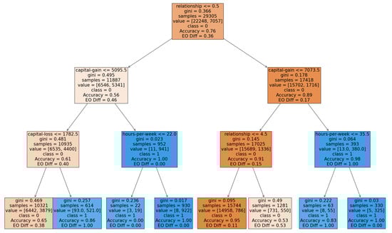
Figure 1.
Example decision tree trained on Adult Income with no sampling.
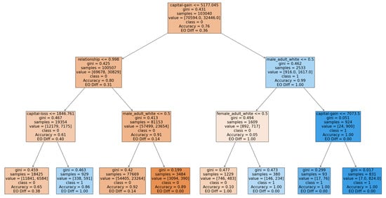
Figure 2.
Decision tree of PC-ADASYN on adult income.
6.1. Comparing Fairness vs. Performance
Comparing oversampling and proportional sampling, the methods’ approaches to augmenting sample size by duplicating existing data rows were straightforward and did not yield substantial improvements in EOD. This outcome makes sense since these methods tend to replicate existing biases, which can potentially exacerbate fairness issues rather than alleviate them. This is evident, in particular, when considering the Adult Income dataset, where the classes are extremely imbalanced. These naïve replication strategies lack the interpolation capacity of PC-SMOTE and PC-ADASYN to adjust samples near decision boundaries, which is crucial for mitigating the bias in the dataset. In contrast, the interpolation strategies used by SMOTE and ADASYN expand the dataset and enhance its diversity. This is particularly effective for samples near decision boundaries, where slight shifts in the features can affect the fairness of predictions significantly. By interpolating between samples, SMOTE and ADASYN effectively move these boundary samples towards more equitable regions of the feature space, thus directly confronting and reducing bias more effectively than methods that increase sample volume without altering data structure. The class generation function (Algorithm 4) also helps increase the overall class distribution. The results of our PC-SMOTE and PC-ADASYN on Adult income also show superiority over the results obtained in [], where the accuracy of 0.59 and SP of 0.17 was obtained. Also, the results of PC-SMOTE and PC-ADASYN show superiority over the results obtained in [], where an EOD of 0.89 and a slightly better accuracy of 0.84.
In examining the results on the German Credit dataset, we observed a trend similar to what was noted in the Adult Income dataset: the no-sampling method has a very high bias regarding EOD. The low SP of 0.07 indicates minimal disparity in the positive prediction rates between the groups, but this in itself is not a good way of measuring fairness since the favored group has more samples than the unfavored one. This has the effect of skewing the calculation of SP since it only counts positive decisions in each group, which are influenced by sample size. One takeaway is the importance of employing multiple fairness metrics to view a model’s impact on all stakeholders comprehensively. For oversampling, we saw an improvement in EOD with a similar SP; this shows that increasing the number of samples for each of the multicategory’s protected attributes improves the fairness with respect to EOD. In addition, the updated SP reflects what it will look like to have a more equal number of samples for each multicategory, unlike in the baseline where the favored group has five times more samples than the unfavored group. The accuracy of proportional sampling drops because the baseline number of samples selected after hyperparameter tuning was insufficient for the model to generalize the unsampled test set, leading to overfitting. The overfitting was confirmed by considering the training accuracy. Interestingly, the model is not trading accuracy for recall like other models, and this gives proportional sampling the highest macro F1.
Regarding fairness, we found an increase in EOD compared with baseline and oversampling. This arises because each multicategory is represented on the same baseline counts. This can improve the model fairness because the model now has a bigger picture of categories and makes better predictions and ultimately fairer decisions. PC-SMOTE and PC-ADASYN play pivotal roles in significantly reducing bias in model predictions. This consistency confirmed the robustness of these methods across different datasets. Notably, neither method compromises accuracy while both enhance fairness, illustrating their effectiveness in handling the trade-offs typically associated with predictive modeling. These results demonstrate the strong interpolation capabilities inherent in PC-SMOTE and PC-ADASYN. These methods effectively reallocate samples within the feature space, especially moving those in underprivileged regions from negative to more positive decision boundaries. Such adjustments are crucial in mitigating biased outcomes and promoting equity in automated decision-making processes. The macro F1 in both models drops compared with the baseline because a higher number of samples is required for the model to perform better on generalization, which this dataset does not support. Specifically, the dataset has 700 samples for class 0 and 300 samples for class 1, which means the test set only has 30 samples for class 1. This small number of samples made both models trade recall for precision in class 1. Notably, we saw a low recall for class 1 which ultimately leads to a low f1-score for class 1 and since macro F1 averages the two f1-scores and treats them equally, this affects the performance of both models in macro F1. Overall, the two models yield a fairer model with good accuracy compared with the baseline and other two sampling methods.
The COMPAS dataset’s evaluation further validates our sampling methods’ effectiveness. The distinct patterns that emerge align with those observed in the Adult Income and German Credit datasets, underscoring the robustness of our findings. Notably, oversampling and proportional sampling techniques have demonstrated substantial improvements in Equalized Odds Difference (EOD) and accuracy, while oversampling also notably improves in SP. This improvement is likely due to the unique composition and balance within the COMPAS dataset, unlike the other datasets in which the classes are imbalanced. The success of oversampling and proportional sampling in this context can be attributed to the balanced nature of the dataset, which allows repeated duplication of existing rows (sampling techniques employed by these methods) to enhance the dataset without introducing a significant skew towards any particular class. This method effectively augments the representation of all classes and the protected attributes in a balanced form, making these techniques particularly effective for datasets where the feature domains contribute equally to predictions and where initial class distributions do not suffer from severe imbalance. This can further be verified from their macro F1 as none of the models is trading precision for recall. The improvement of SP in oversampling can be attributed to the higher number of samples in oversampling in comparison with proportional sampling. Regarding PC-SMOTE and PC-ADASYN, these algorithms show an improvement over baseline in both accuracy and EOD. These trends follow those in the previous results. One notable thing in this results in the large drop in SP which can be attributed to our new label that was generated to make the dataset to be skewed towards the negative class. These results show the difficulty in optimizing for two or more fairness metrics at a time and how this optimization can affect each other.
6.2. Impact of Tree Depth on Fairness and Accuracy
In this study, the impact of decision tree depth on model performance was also investigated, specifically examining how variations in tree depth influence accuracy and EOD. Understanding the depth’s effect is crucial as it provides insight into the effects ranging from underfitting to overfitting and helps identify the optimal complexity level at which both accuracy and fairness are maximized. Initially, the decision tree was allowed to grow without constraints to its full depth which on average was about 30 branches. The tree was then examined visually to deduce the maximum depth excluding the nonsplitting branches. To analyze the effects of tree depth systematically, the maximum depth of the trees was allowed to vary from 1 to 30. Each depth limit was evaluated using ten-fold cross-validation to ensure the robustness and generalizability of the findings.
For each configuration of tree depth, the accuracy and EOD were measured on the test set. Additionally, 95% confidence intervals were calculated for the metrics across the ten folds. This statistical analysis highlighted the depth at which the decision tree balanced the trade-off between accuracy and fairness while also considering the underlying statistical bias–variance tradeoff. By doing so, it was possible to pinpoint the “sweet spot”—a delicate point where the decision tree maintains high predictive accuracy without compromising on fairness, effectively countering the often-cited trade-off presented in previous literature. Figure 3, Figure 4, Figure 5, Figure 6 and Figure 7 show the plots of accuracy and EOD against maximum depth for each of the five sampling methods on the Adult Income dataset.
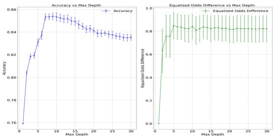
Figure 3.
Plots of Adult Income using no sampling, showing accuracy and EOD with 95% confidence intervals against the maximum tree depth ranging from 1 to 30.
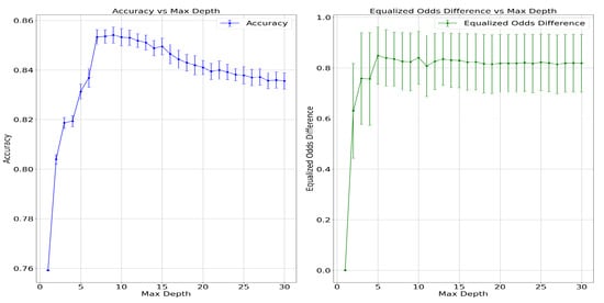
Figure 4.
Plots of Adult Income using oversampling, showing accuracy and EOD with 95% confidence intervals against the maximum tree depth ranging from 1 to 30.
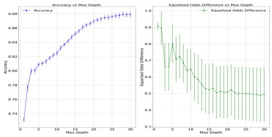
Figure 5.
Plots of Adult Income using proportional sampling, showing accuracy and EOD with 95% confidence intervals against the maximum tree depth ranging from 1 to 30.
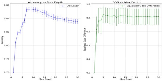
Figure 6.
Plots of Adult Income using PC-SMOTE, showing accuracy and EOD with 95% confidence intervals against the maximum tree depth ranging from 1 to 30.
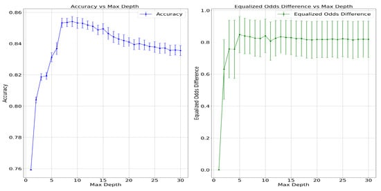
Figure 7.
Plots of Adult Income using PC-ADASYN, showing accuracy and EOD with 95% confidence intervals against the maximum tree depth ranging from 1 to 30.
Based on results such as those shown in Figure 3 and Figure 4, there is a notable initial increase in accuracy as maximum depth increases for both the no-sampling and the oversampling methods. However, both methods exhibit a decline in accuracy from a depth of 10 onwards, suggesting the onset of overfitting. Correspondingly, the EOD decreases sharply with increasing depth up to about depth 10, beyond which it stabilizes. This pattern indicates that while deeper trees initially improve fairness, they eventually reach a threshold beyond which no further gains are observed. Recalling that the fairness goal was to minimize EOD, a key observation is that setting the maximum depth between three and five strikes an optimal balance between achieving high accuracy and maintaining low EOD.
When considering the results shown in Figure 5, the proportional sampling method continually increases accuracy with tree depth, peaking at a depth of about 26. Conversely, the EOD initially increases before decreasing and stabilizing at a depth of around 15. The wide confidence intervals observed in the EOD metric suggest significant variability in fairness outcomes. This finding underscores the importance of selecting a depth that minimizes variability in fairness while maximizing accuracy.
Figure 6 and Figure 7, representing the results using PC-SMOTE and PC-ADASYN, respectively, exhibit slight downward trends in accuracy, which improve briefly before descending again—a pattern indicative of overfitting at greater depths. EOD metrics for these methods show initial stability at lower depths, surge at mid-level depths, and decline, suggesting complex interactions between synthetic sample generation and decision boundary delineation. Given these observations, a maximum depth of 3 was chosen for our experiments, as it represents a “sweet spot” where both accuracy and EOD are optimized.
Given these results, one conclusion is to challenge the often presumed trade-off between accuracy and fairness by demonstrating that our PC-ADASYN method consistently outperforms baselines across all three datasets in terms of both accuracy and fairness. This finding is significant, as it suggests enhancing model fairness without sacrificing accuracy with appropriate sampling methods and model tuning is possible. However, our analysis also reveals scenarios where adjustments to model complexity, specifically the maximum depth of decision trees, can enhance accuracy at the expense of fairness, as indicated by increases in Equalized Odds Difference (EOD). It is expected, however, that coupling sampling methods with inprocessing methods such as fairness-based regularization may offset these effects. These decisions highlight researchers’ discretionary power in balancing model performance metrics depending on their study’s specific objectives and constraints. The quantity of sample and time complexity is like every other sampling method. As the sample quantity increase, the time complexity increases but overall, the sampling methods have the same time complexity as their underlying algorithms because they have the same functionality.
Moreover, our results underscore the complexities of simultaneously optimizing multiple fairness metrics. For instance, efforts to improve Statistical Parity (SP) by favoring more positive predictions for each protected group in the COMPAS dataset led to an inadvertent reduction in negative predictions. This shift adversely impacted the False Positive Rate (FPR), a component of EOD, thereby worsening the EOD metric as SP improved. This phenomenon illustrates the inherent mathematical tensions between fairness metrics, where optimizing one can detrimentally affect another. The COMPAS dataset, with its nearly balanced class distribution, provides a concrete example of how dataset characteristics can influence the behavior of fairness metrics. Optimizing SP in this context implies a skewed measurement of fairness, particularly where inherent differences exist between groups in protected attributes. This is supported by literature indicating that SP may not adequately account for group differences, potentially leading to misleading conclusions about a model’s fairness [].
7. Limitations and Future Work
The very nature of this study is such that it is not possible to address all of the issues surrounding fairness and the so-called fairness–performance tradeoff. As such, there exist limitations in the work reported here. Even so, it is our hope and intent for the work reported here to suggest additional avenues of exploration in this important area.
One limitation of this study is that our sampling method was not specifically designed to optimize for arbitrary fairness metrics. Stated another way, since often inherent tradeoffs exist between the available set of fairness metrics, the decision was made to focus on an approach that was metric agnostic, recognizing that the results could have differed for other metrics. This is also part of the reason why we saw different behaviors between EOD and SP.
In addition, it is acknowledged that, while the underlying ML method should not be relevant to the method proposed, this has not actually been tested. Therefore, in the future, this research will be extended by considering the impacts of other ML algorithms such as logistic regression, fuzzy ID3, K-nearest neighbor, and ensemble methods such as random forests or gradient-boosted trees to assess the generalizability of our new sampling methods. The purpose of such a study would be to verify that our methods are independent of the ML algorithm employed. Furthermore, this would help validate whether the observed improvements in fairness and accuracy are model-specific or can be universally applied.
Additionally, it is acknowledged that only three distinct datasets were considered—datasets that have been studied extensively in the field. This raises a concern that methods are being tailored to these data rather than addressing the broader issue of fairness in ML. To address this, experiments with larger and more diverse datasets are planned to provide deeper insights into the scalability and robustness of our techniques. Another area for future work is to refine our multicategory sampling approach by incorporating more granular subdivisions of protected categories, potentially revealing subtler biases and providing a more nuanced understanding of fairness.
Finally, it is recognized that alternative methods have been proposed for bias mitigation, and these methods have not been studied in this work at all. Future work would entail comparisons with more sampling strategies. A more direct comparison of the proposed methods with inprocessing and postprocessing methods will be conducted. For example, incorporating inprocessing methods, such as regularization [], or a postprocessing method, such as the Randomized Threshold Optimizer [], will be explored as possible means to obtain further improvements in both fairness and performance.
8. Conclusions
In this study, the issue of bias in ML predictions was investigated, and a method was developed based on combining protected variables into a new multicategory. In particular, the focus was on the question that has been suggested in the literature of a bias–performance tradeoff and seeking a method to mitigate this tradeoff. The proposed new multicategory approach reflects the multifaceted identity of individuals, acknowledging the complex interplay of attributes that define real-world scenarios. Given the inherent imbalance in this multicategory, four sampling methods tailored to these complex categorizations, rather than traditional class labels, were developed. For purposes of applying a baseline classifier, decision trees were trained, and the effectiveness of these methods was evaluated using three datasets that are often employed in fairness studies. The performance of the methods was compared against baseline methods of no sampling, using accuracy, macro F1, Equalized Odds Difference (EOD), and Statistical Parity (SP) as the evaluation metrics.
The results of the experiments indicate that two of the newly developed sampling techniques—PC-SMOTE and PC-ADASYN—successfully enhance fairness without compromising accuracy. Remarkably, in some cases, these methods also improved accuracy, thus providing evidence counter to the popular claims of a fairness–performance tradeoff. Further analysis of the impact of maximum tree depth on model performance revealed that, while increasing depth initially boosts accuracy, it eventually leads to a decline. Conversely, increasing depth adversely affects fairness, highlighting the challenge of balancing complexity with equity. However, optimal tree depths were identified that simultaneously enhance accuracy and EOD, underscoring the possibility of achieving equity without sacrificing performance.
Ultimately, these findings challenge prevailing notions of an implicit performance–fairness tradeoff within bias mitigation research, suggesting that carefully designed bias mitigation strategies have the ability to sidestep this trade-off. Our approach sets a new precedent for developing more equitable predictive algorithms by redefining how protected attributes are utilized in model training.
Author Contributions
Conceptualization, G.P. and J.S.; formal analysis, G.P. and J.S.; investigation, G.P.; methodology, G.P.; software, G.P.; supervision, J.S.; validation, G.P. and J.S.; visualization, G.P.; writing—original draft, G.P.; writing—review and editing, J.S. All authors have read and agreed to the published version of the manuscript.
Funding
This research received no external funding.
Data Availability Statement
The datasets and code implemented in this research work have been uploaded to https://github.com/horlahsunbo/New-folder (accessed on 10 June 2024).
Conflicts of Interest
The authors declare no conflicts of interest.
References
- Maina, I.W.; Belton, T.D.; Ginzberg, S.; Singh, A.; Johnson, T.J. A decade of studying implicit racial/ethnic bias in healthcare providers using the implicit association test. Soc. Sci. Med. 2018, 199, 219–229. [Google Scholar] [CrossRef]
- Salimi, B.; Rodriguez, L.; Howe, B.; Suciu, D. Causal database repair for algorithmic fairness. In Proceedings of the 2019 International Conference on Management of Data, Amsterdam, The Netherlands, 30 June–5 July 2019; pp. 793–810. [Google Scholar]
- Kordzadeh, N.; Ghasemaghaei, M. Algorithmic Bias: Review, Synthesis, and Future Research Directions. Eur. J. Inf. Syst. 2022, 31, 388–409. [Google Scholar] [CrossRef]
- Pessach, D.; Shmueli, E. A review on fairness in machine learning. ACM Comput. Surv. 2022, 55, 1–44. [Google Scholar] [CrossRef]
- Aghaei, S.; Azizi, M.J.; Vayanos, P. Learning optimal and fair decision trees for non-discriminative decision-making. Proc. AAAI Conf. Artif. Intell. 2019, 33, 1418–1426. [Google Scholar] [CrossRef]
- Kamiran, F.; Calders, T. Data preprocessing techniques for classification without discrimination. Knowl. Inf. Syst. 2012, 33, 1–33. [Google Scholar] [CrossRef]
- Calmon, F.; Wei, D.; Vinzamuri, B.; Ramamurthy, K.N.; Varshney, K.R. Optimized pre-processing for discrimination prevention. In Proceedings of the Advances in Neural Information Processing Systems, Long Beach, CA, USA, 4–9 December 2017. [Google Scholar]
- Shahbazi, N.; Lin, Y.; Asudeh, A.; Jagadish, H.V. Representation bias in data: A survey on identification and resolution techniques. ACM Comput. Surv. 2023, 55, 1–39. [Google Scholar] [CrossRef]
- Chen, Z.; Zhang, J.M.; Sarro, F.; Harman, M. A comprehensive empirical study of bias mitigation methods for machine learning classifiers. ACM Trans. Softw. Eng. Methodol. 2023, 32, 1–30. [Google Scholar] [CrossRef]
- Perzynski, A.; Berg, K.A.; Thomas, C.; Cemballi, A.; Smith, T.; Shick, S.; Gunzler, D.; Sehgal, A.R. Racial discrimination and economic factors in redlining of Ohio neighborhoods. Bois Rev. Soc. Sci. Res. Race 2023, 20, 293–309. [Google Scholar] [CrossRef]
- Steil, J.P.; Albright, L.; Rugh, J.S.; Massey, D.S. The social structure of mortgage discrimination. Hous. Stud. 2018, 33, 759–776. [Google Scholar] [CrossRef]
- Salgado, J.F.; Moscoso, S.; García-Izquierdo, A.L.; Anderson, N.R. Shaping Inclusive Workplaces through Social Dialogue; Springer: Berlin/Heidelberg, Germany, 2017. [Google Scholar]
- Leavy, S.; Meaney, G.; Wade, K.; Greene, D. Mitigating gender bias in machine learning data sets. In Proceedings of the Bias and Social Aspects in Search and Recommendation: First International Workshop, BIAS 2020, Lisbon, Portugal, 14 April 2020; pp. 12–26. [Google Scholar]
- Hort, M.; Chen, Z.; Zhang, J.M.; Harman, M.; Sarro, F. Bias mitigation for machine learning classifiers: A comprehensive survey. ACM J. Responsible Comput. 2023, 1, 1–52. [Google Scholar] [CrossRef]
- Fahse, T.; Huber, V.; van Giffen, B. Managing bias in machine learning projects. In Innovation Through Information Systems: Volume II: A Collection of Latest Research on Technology Issues; Springer: Berlin/Heidelberg, Germany, 2021; pp. 94–109. [Google Scholar]
- Zhang, Z.; Neill, D.B. Identifying Significant Predictive Bias in Classifiers. arXiv 2017, arXiv:1611.08292. [Google Scholar] [CrossRef]
- Zheng, Z.; Cai, Y.; Li, Y. Oversampling method for imbalanced classification. Comput. Inform. 2015, 34, 1017–1037. [Google Scholar]
- Chawla, N.V.; Bowyer, K.W.; Hall, L.O.; Kegelmeyer, W.P. SMOTE: Synthetic minority over-sampling technique. J. Artif. Intell. Res. 2002, 16, 321–357. [Google Scholar] [CrossRef]
- He, H.; Bai, Y.; Garcia, E.A.; Li, S. ADASYN: Adaptive synthetic sampling approach for imbalanced learning. In Proceedings of the 2008 IEEE International Joint Conference on Neural Networks (IEEE World Congress on Computational Intelligence), Hong Kong, China, 1–8 June 2008; pp. 1322–1328. [Google Scholar]
- Janssen, P.; Sadowski, B.M. Bias in Algorithms: On the trade-off between accuracy and fairness. In Proceedings of the 23rd Biennial Conference of the International Telecommunications Society, Gothenburg, Sweden, 21–23 June 2021. [Google Scholar]
- Hardt, M.; Price, E.; Srebro, N. Equality of opportunity in supervised learning. In Proceedings of the Advances in Neural Information Processing Systems, Barcelona, Spain, 5–10 December 2016. [Google Scholar]
- Kamishima, T.; Akaho, S.; Asoh, H.; Sakuma, J. Fairness-aware classifier with prejudice remover regularizer. In Proceedings of the Machine Learning and Knowledge Discovery in Databases: European Conference, ECML PKDD 2012, Bristol, UK, 24–28 September 2012; pp. 35–50. [Google Scholar]
- Calders, T.; Žliobaitè, I. Why unbiased computational processes can lead to discriminative decision procedures. In Discrimination and Privacy in the Information Society: Data Mining and Profiling in Large Databases; Springer: Berlin/Heidelberg, Germany, 2013; pp. 23–33. [Google Scholar]
- Burt, A. How to Fight Discrimination in AI. Harvard Business Review. 2020. Available online: https://hbr.org/2020/08/how-to-fight-discrimination-in-ai (accessed on 12 July 2024).
- Siegler, A.; Admussen, W. Discovering Racial Discrimination by the Police. Northwestern Univ. Law Rev. 2021, 115, 987–1054. [Google Scholar]
- Grabowicz, P.; Perello, N.; Mishra, A. How to Train Models that Do Not Propagate Discrimination? Equate and Machine Learning Blog, University of Massachusets, Amherst. 2022. Available online: https://groups.cs.umass.edu/equate-ml/2022/04/07/how-to-train-models-that-do-not-propagate-discrimination/ (accessed on 12 July 2024).
- Khani, F.; Liang, P. From Discrimination in Machine Learning to Discrimination in Law, Part 1: Disparate Treatment. Stanford AI Lab Blog. 2022. Available online: https://ai.stanford.edu/blog/discrimination_in_ML_and_law/ (accessed on 12 July 2024).
- Shahriari, K.; Shahriari, M. IEEE standard review—Ethically aligned design: A vision for prioritizing human wellbeing with artificial intelligence and autonomous systems. In Proceedings of the IEEE Canada International Humanitarian Technology Conference (IHTC), Toronto, ON, Canada, 21–22 July 2017; pp. 197–201. [Google Scholar]
- European Commission; Directorate-General for Communications Networks, Content and Technology. Ethics Guidelines for Trustworthy AI. Publications Office. 2019. Available online: https://op.europa.eu/en/publication-detail/-/publication/d3988569-0434-11ea-8c1f-01aa75ed71a1/language-en/format-PDF/source-337437547 (accessed on 10 June 2024).
- Ebers, M.; Hoch, V.R.S.; Rosenkranz, F.; Ruschemeier, H.; Steinrötter, B. The European Commission’s Proposal for an Artificial Intelligence Act–A Critical Assessment by Members of the Robotics and AI Law Society (RAILS). J 2021, 4, 589–603. [Google Scholar] [CrossRef]
- Hajian, S.; Domingo-Ferrer, J. A methodology for direct and indirect discrimination prevention in data mining. IEEE Trans. Knowl. Data Eng. 2012, 25, 1445–1459. [Google Scholar] [CrossRef]
- Fish, B.; Kun, J.; Lelkes, Á.D. A confidence-based approach for balancing fairness and accuracy. In Proceedings of the 2016 SIAM International Conference on Data Mining, Miami, FL, USA, 5–7 May 2016; pp. 144–152. [Google Scholar]
- Hajian, S. Simultaneous Discrimination Prevention and Privacy Protection in Data Publishing and Mining. arXiv 2013, arXiv:1306.6805. [Google Scholar] [CrossRef]
- Sondeck, L.P.; Laurent, M.; Frey, V. The Semantic Discrimination Rate Metric for Privacy Measurements which Questions the Benefit of t-closeness over l-diversity. In Proceedings of the 14th International Conference on Security and Cryptography, Madrid, Spain, 24–26 July 2017; Volume 6, pp. 285–294. [Google Scholar]
- Ruggieri, S. Using t-closeness anonymity to control for non-discrimination. Trans. Data Priv. 2014, 2, 99–129. [Google Scholar]
- Romano, Y.; Bates, S.; Candes, E. Achieving equalized odds by resampling sensitive attributes. In Proceedings of the Advances in Neural Information Processing Systems, Online, 6–12 December 2020; pp. 361–371. [Google Scholar]
- Peng, K.; Chakraborty, J.; Menzies, T. Fairmask: Better fairness via model-based rebalancing of protected attributes. IEEE Trans. Softw. Eng. 2022, 49, 2426–2439. [Google Scholar] [CrossRef]
- Dhar, P.; Gleason, J.; Roy, A.; Castillo, C.D.; Chellappa, R. PASS: Protected attribute suppression system for mitigating bias in face recognition. In Proceedings of the IEEE/CVF International Conference on Computer Vision, Montreal, QC, Canada, 10–17 October 2021; pp. 15087–15096. [Google Scholar]
- Krasanakis, E.; Spyromitros-Xioufis, E.; Papadopoulos, S.; Kompatsiaris, Y. Adaptive sensitive reweighting to mitigate bias in fairness-aware classification. In Proceedings of the World Wide Web Conference, Lyon, France, 23–27 April 2018; pp. 853–862. [Google Scholar]
- Rančić, S.; Radovanović, S.; Delibašić, B. Investigating oversampling techniques for fair machine learning models. In Proceedings of the Decision Support Systems XI: Decision Support Systems, Analytics and Technologies in Response to Global Crisis Management: 7th International Conference on Decision Support System Technology, ICDSST 2021, Loughborough, UK, 26–28 May 2021; Springer: Berlin/Heidelberg, Germany, 2021; pp. 110–123. [Google Scholar]
- Yan, S.; te Kao, H.; Ferrara, E. Fair class balancing: Enhancing model fairness without observing sensitive attributes. In Proceedings of the 29th ACM International Conference on Information & Knowledge Management, Virtual Event, Ireland, 19–23 October 2010; pp. 1715–1724. [Google Scholar]
- HuZhang, B.; Lemoine, B.; Mitchell, M. Mitigating unwanted biases with adversarial learning. In Proceedings of the AAAI/ACM Conference on AI, Ethics, and Society, New Orleans, LA, USA, 2–3 February 2018; pp. 335–340. [Google Scholar]
- Celis, L.E.; Huang, L.; Keswani, V.; Vishno, N.K. Classification with fairness constraints: A meta-algorithm with provable guarantees. In Proceedings of the Conference on Fairness, Accountability, and Transparency, Atlanta, GA, USA, 29–31 January 2019; pp. 319–328. [Google Scholar]
- Zafar, M.B.; Valera, I.; Rodriguez, M.G.; Gummadi, K.P. Fairness beyond disparate treatment & disparate impact: Learning classification without disparate mistreatment. In Proceedings of the 26th International Conference on World Wide Web, Perth, Australia, 3–7 April 2017; pp. 1171–1180. [Google Scholar]
- Agarwal, A.; Beygelzimer, A.; Dudík, M.; Langford, J.; Wallach, H. A reductions approach to fair classification. In Proceedings of the International Conference on Machine Learning, Stockholm, Sweden, 10–15 July 2018; pp. 60–69. [Google Scholar]
- Lowy, A.; Baharlouei, S.; Pavan, R.; Razaviyayn, M.; Beirami, A. A Stochastic Optimization Framework for Fair Risk Minimization. Trans. Mach. Learn. Res. 2022. [Google Scholar] [CrossRef]
- Spinelli, I.; Scardapane, S.; Hussain, A.; Uncini, A. Fairdrop: Biased edge dropout for enhancing fairness in graph representation learning. IEEE Trans. Artif. Intell. 2021, 3, 344–354. [Google Scholar] [CrossRef]
- Hort, M.; Zhang, J.M.; Sarro, F.; Harman, M. Fairea: A model behaviour mutation approach to benchmarking bias mitigation methods. In Proceedings of the 29th ACM Joint Meeting on European Software Engineering Conference and Symposium on the Foundations of Software Engineering, Athens, Greece, 23–28 August 2012; pp. 994–1006. [Google Scholar]
- Bhaskaruni, D.; Hu, H.; Lan, C. Improving Prediction Fairness via Model Ensemble. In Proceedings of the IEEE 31st International Conference on Tools with Artificial Intelligence (ICTAI), Portland, OR, USA, 4–6 November 2019; pp. 1810–1814. [Google Scholar]
- Iosifidis, V.; Fetahu, B.; Ntoutsi, E. Fae: A fairness-aware ensemble framework. In Proceedings of the IEEE International Conference on Big Data (Big Data), Los Angeles, CA, USA, 9–12 December 2019; pp. 1375–1380. [Google Scholar]
- Dwork, C.; Hardt, M.; Pitassi, T.; Reingold, O.; Zemel, R. Fairness through awareness. In Proceedings of the 3rd Innovations in Theoretical Computer Science Conference, Cambridge, MA, USA, 8–10 January 2012; pp. 214–226. [Google Scholar]
- Pleiss, G.; Raghavan, M.; Wu, F.; Kleinberg, J.; Weinberger, K.Q. On fairness and calibration. In Proceedings of the Advances in Neural Information Processing Systems, Long Beach, CA, USA, 4–8 December 2017. [Google Scholar]
- Karimi-Haghighi, M.; Castillo, C. Enhancing a recidivism prediction tool with machine learning: Effectiveness and algorithmic fairness. In Proceedings of the Eighteenth International Conference on Artificial Intelligence and Law, São Paulo, Brazil, 21–25 June 2017; pp. 210–214. [Google Scholar]
- Friedler, S.A.; Scheidegger, C.; Venkatasubramanian, S. The (im)possibility of fairness: Different value systems require different mechanisms for fair decision making. Commun. ACM 2021, 64, 136–143. [Google Scholar] [CrossRef]
- García, V.; Sánchez, J.S.; Mollineda, R.A. On the effectiveness of preprocessing methods when dealing with different levels of class imbalance. Knowl.-Based Syst. 2012, 25, 13–21. [Google Scholar] [CrossRef]
- Breiman, L. Classification and Regression Trees; Routledge: London, UK, 2017. [Google Scholar]
- Pedregosa, F.; Varoquaux, G.; Gramfort, A.; Michel, V.; Thirion, B.; Grisel, O.; Blondel, M.; Prettenhofer, P.; Weiss, R.; Dubourg, V.; et al. Scikit-learn: Machine Learning in Python. J. Mach. Learn. Res. 2011, 12, 2825–2830. [Google Scholar]
- Kelly, M.; Longjohn, R.; Nottingham, K. The UCI Machine Learning Repository. 2024. Available online: https://archive.ics.uci.edu (accessed on 10 June 2024).
- Becker, B.; Kohavi, R. Adult. UCI Machine Learning Repository. 1996. Available online: https://archive.ics.uci.edu/dataset/2/adult (accessed on 10 June 2024). [CrossRef]
- Hofmann, H.; Statlog (German Credit Data). UCI Machine Learning Repository. 1994. Available online: https://archive.ics.uci.edu/dataset/144/statlog+german+credit+data (accessed on 10 June 2024). [CrossRef]
- Dressel, J.; Farid, H. The accuracy, fairness, and limits of predicting recidivism. Sci. Adv. 2018, 4, eaao5580. [Google Scholar] [CrossRef]
- Huang, Q.; Mao, J.; Liu, Y. An improved grid search algorithm of SVR parameters optimization. In Proceedings of the 2012 IEEE 14th International Conference on Communication Technology, Chengdu, China, 9–11 November 2012; pp. 1022–1026. [Google Scholar]
- Caton, S.; Haas, C. Fairness in machine learning: A survey. ACM Comput. Surv. 2023, 56, 1–38. [Google Scholar] [CrossRef]
- Alabdulmohsin, I.; Lucic, M. A Near-Optimal Algorithm for Debiasing Trained Machine Learning Models. In Proceedings of the 35th Conference on Neural Information Processing Systems, Online, 6–14 December 2021. [Google Scholar]
Disclaimer/Publisher’s Note: The statements, opinions and data contained in all publications are solely those of the individual author(s) and contributor(s) and not of MDPI and/or the editor(s). MDPI and/or the editor(s) disclaim responsibility for any injury to people or property resulting from any ideas, methods, instructions or products referred to in the content. |
© 2024 by the authors. Licensee MDPI, Basel, Switzerland. This article is an open access article distributed under the terms and conditions of the Creative Commons Attribution (CC BY) license (https://creativecommons.org/licenses/by/4.0/).