
FPGA Implementation of Pillar-Based Object Classification for Autonomous Mobile Robot


Abstract
:1. Introduction
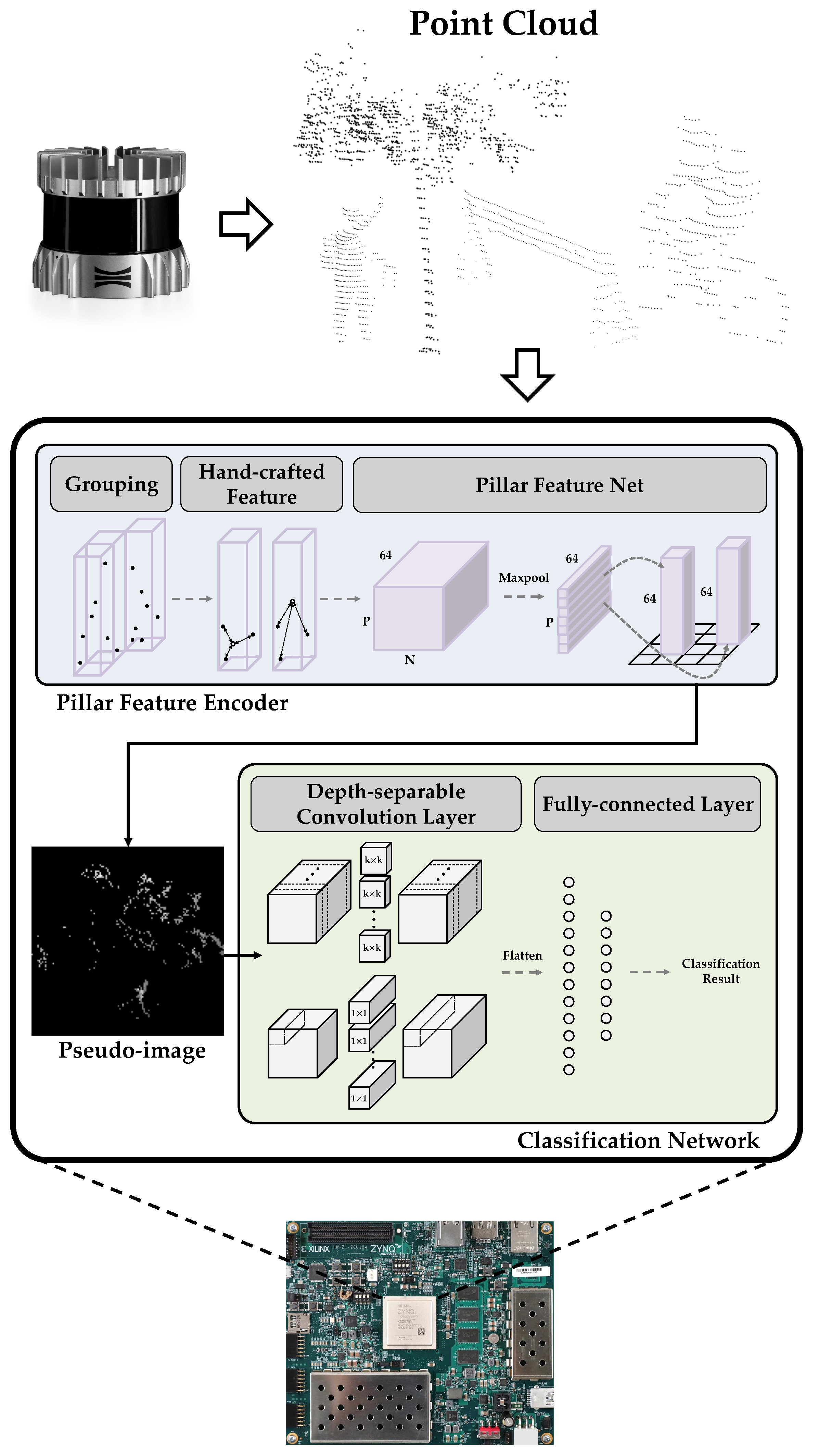
2. Proposed System
2.1. PFE
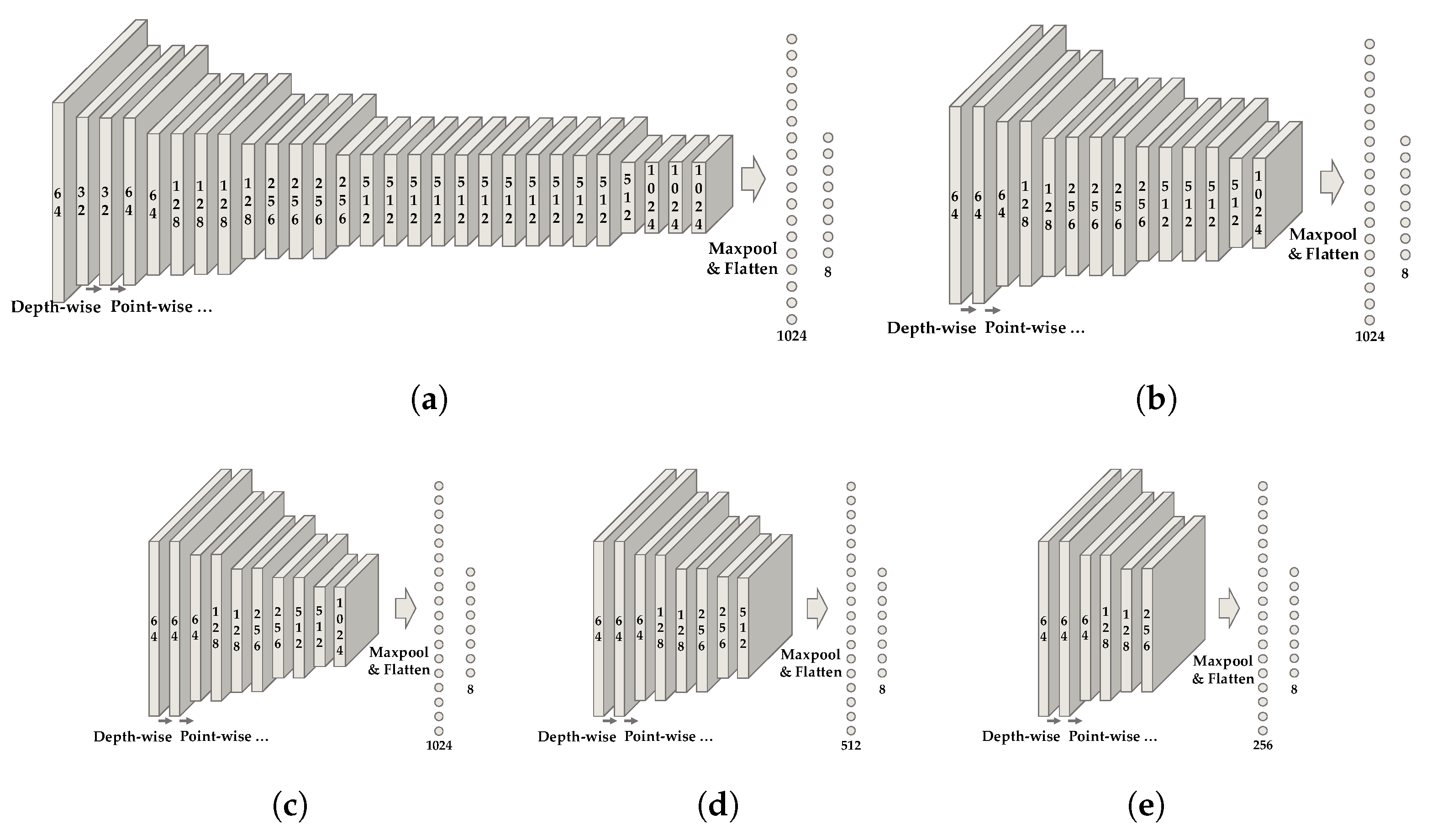
2.2. Classification Network
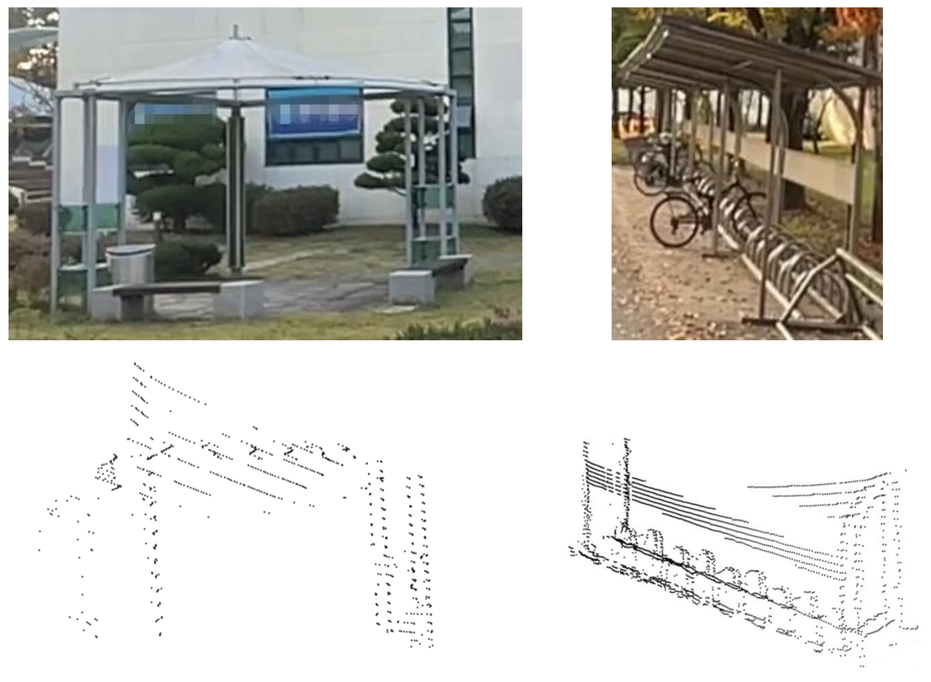
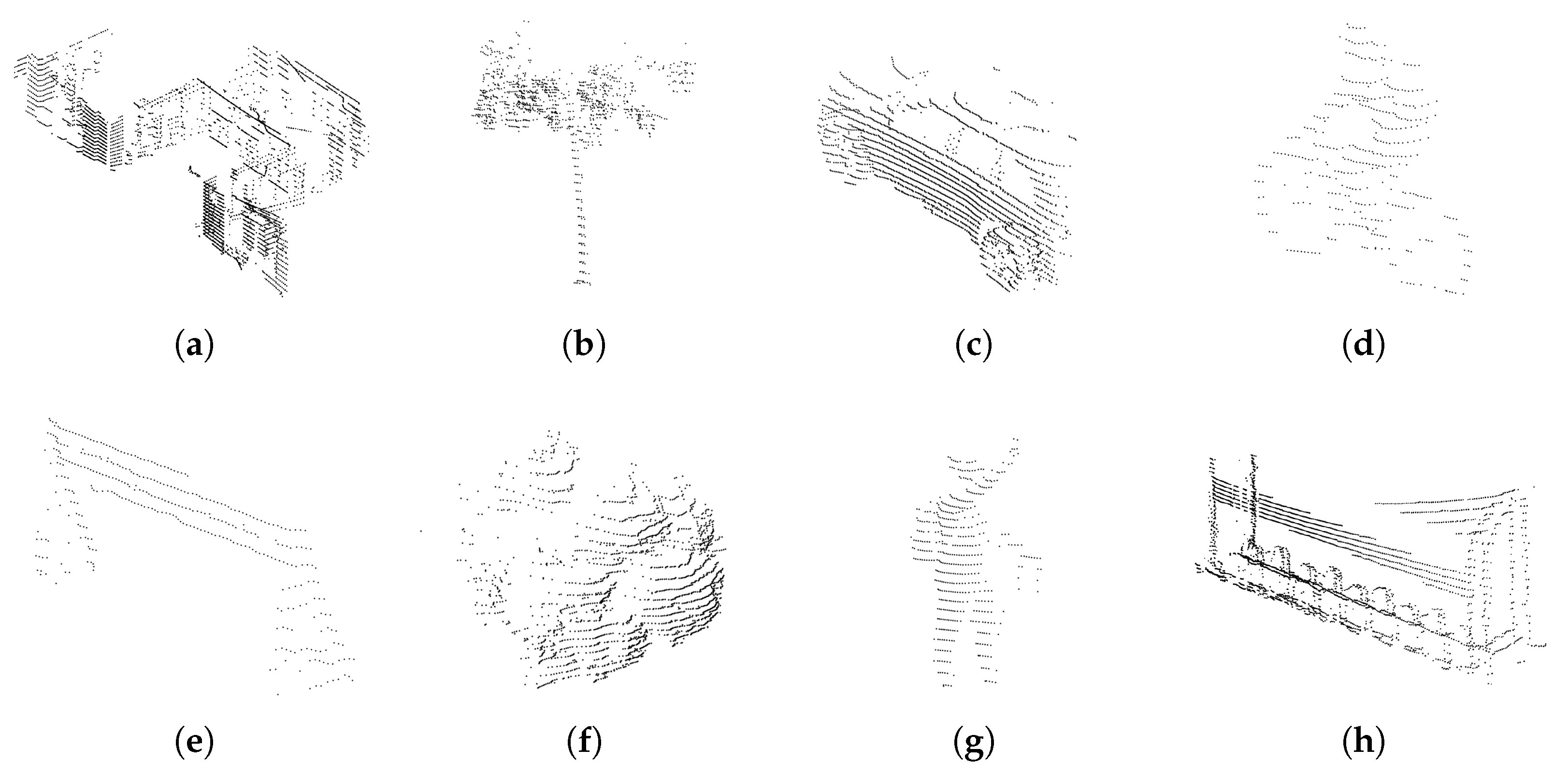
2.3. Dataset
2.4. Performance Evaluation
3. Implementation of Acceleration System
3.1. Quantization
3.2. System Architecture
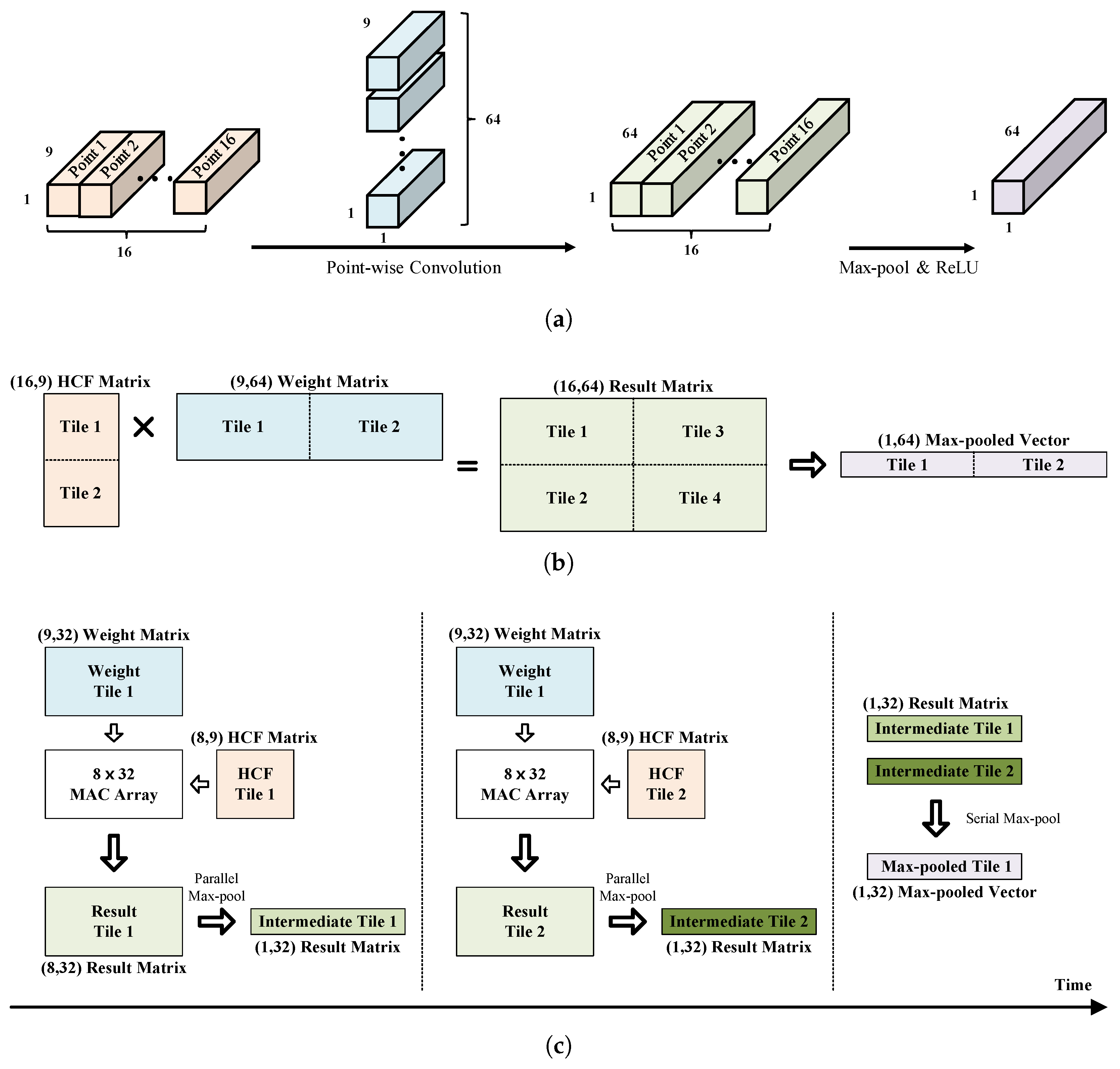
3.3. PFE Hardware Architecture
3.4. Classification Network Accelerator Using FINN
4. Implementation Results
5. Conclusions
Author Contributions
Funding
Institutional Review Board Statement
Informed Consent Statement
Data Availability Statement
Conflicts of Interest
References
- Varlamov, O. “Brains” for Robots: Application of the Mivar Expert Systems for Implementation of Autonomous Intelligent Robots. Big Data Res. 2021, 25, 100241. [Google Scholar] [CrossRef]
- Liu, Y.; Li, Z.; Liu, H.; Kan, Z. Skill Transfer Learning for Autonomous Robots and Human–robot Cooperation: A Survey. Robot. Auton. Syst. 2020, 128, 103515. [Google Scholar] [CrossRef]
- Yoshioka, M.; Suganuma, N.; Yoneda, K.; Aldibaja, M. Real-time Object Classification for Autonomous Vehicle using LIDAR. In Proceedings of the 2017 International Conference on Intelligent Informatics and Biomedical Sciences (ICIIBMS), Okinawa, Japan, 24–26 November 2017; pp. 210–211. [Google Scholar]
- Gao, H.; Cheng, B.; Wang, J.; Li, K.; Zhao, J.; Li, D. Object Classification using CNN-based Fusion of Vision and LIDAR in Autonomous Vehicle Environment. IEEE Trans. Ind. Inform. 2018, 14, 4224–4231. [Google Scholar] [CrossRef]
- Zhou, Y.; Liu, L.; Zhao, H.; López-Benítez, M.; Yu, L.; Yue, Y. Towards Deep Radar Perception for Autonomous Driving: Datasets, Methods, and Challenges. Sensors 2022, 22, 4208. [Google Scholar] [CrossRef] [PubMed]
- Su, H.; Maji, S.; Kalogerakis, E.; Learned-Miller, E. Multi-view Convolutional Neural Networks for 3D Shape Recognition. In Proceedings of the IEEE International Conference on Computer Vision, Santiago, Chile, 7–13 December 2015; pp. 945–953. [Google Scholar]
- Hoang, L.; Lee, S.H.; Lee, E.J.; Kwon, K.R. GSV-NET: A Multi-modal Deep Learning Network for 3D Point Cloud Classification. Appl. Sci. 2022, 12, 483. [Google Scholar] [CrossRef]
- Qi, C.R.; Su, H.; Mo, K.; Guibas, L.J. Pointnet: Deep Learning on Point Sets for 3D Classification and Segmentation. In Proceedings of the IEEE Conference on Computer Vision and Pattern Recognition, Honolulu, HI, USA, 21–26 July 2017; pp. 652–660. [Google Scholar]
- Zhou, Y.; Tuzel, O. Voxelnet: End-to-end Learning for Point Cloud based 3D Object Detection. In Proceedings of the IEEE Conference on Computer Vision and Pattern Recognition, Salt Lake City, UT, USA, 18–22 June 2018; pp. 4490–4499. [Google Scholar]
- Bhanushali, D.; Relyea, R.; Manghi, K.; Vashist, A.; Hochgraf, C.; Ganguly, A.; Kwasinski, A.; Kuhl, M.E.; Ptucha, R. LiDAR-camera Fusion for 3D Object Detection. Electron. Imaging 2020, 32, 1–9. [Google Scholar] [CrossRef]
- Yan, Y.; Mao, Y.; Li, B. Second: Sparsely Embedded Convolutional Detection. Sensors 2018, 18, 3337. [Google Scholar] [CrossRef] [PubMed]
- Lang, A.H.; Vora, S.; Caesar, H.; Zhou, L.; Yang, J.; Beijbom, O. Pointpillars: Fast encoders for Object Detection from Point Clouds. In Proceedings of the IEEE/CVF Conference on Computer Vision and Pattern Recognition, Long Beach, CA, USA, 15–20 June 2019; pp. 12697–12705. [Google Scholar]
- Lis, K.; Kryjak, T. PointPillars Backbone Type Selection for Fast and Accurate LiDAR Object Detection. In Proceedings of the International Conference on Computer Vision and Graphics, Warsaw, Poland, 19–21 September 2022; Springer: Berlin/Heidelberg, Germany, 2022; pp. 99–119. [Google Scholar]
- Shu, X.; Zhang, L. Research on PointPillars Algorithm based on Feature-Enhanced Backbone Network. Electronics 2024, 13, 1233. [Google Scholar] [CrossRef]
- Wang, Y.; Han, X.; Wei, X.; Luo, J. Instance Segmentation Frustum–PointPillars: A Lightweight Fusion Algorithm for Camera–LiDAR Perception in Autonomous Driving. Mathematics 2024, 12, 153. [Google Scholar] [CrossRef]
- Agashe, P.; Lavanya, R. Object Detection using PointPillars with Modified DarkNet53 as Backbone. In Proceedings of the 2023 IEEE 20th India Council International Conference (INDICON), Hyderabad, India, 14–17 December 2023; pp. 114–119. [Google Scholar]
- Choi, Y.; Kim, B.; Kim, S.W. Performance Analysis of PointPillars on CPU and GPU Platforms. In Proceedings of the 2021 36th International Technical Conference on Circuits/Systems, Computers and Communications (ITC-CSCC), Jeju, Republic of Korea, 27–30 June 2021; pp. 1–4. [Google Scholar]
- Silva, A.; Fernandes, D.; Névoa, R.; Monteiro, J.; Novais, P.; Girão, P.; Afonso, T.; Melo-Pinto, P. Resource-constrained onboard Inference of 3D Object Detection and Localisation in Point Clouds Targeting Self-driving Applications. Sensors 2021, 21, 7933. [Google Scholar] [CrossRef] [PubMed]
- Stanisz, J.; Lis, K.; Gorgon, M. Implementation of the Pointpillars Network for 3D Object Detection in Reprogrammable Heterogeneous Devices using FINN. J. Signal Process. Syst. 2022, 94, 659–674. [Google Scholar] [CrossRef]
- Li, Y.; Zhang, Y.; Lai, R. TinyPillarNet: Tiny Pillar-based Network for 3D Point Cloud Object Detection at Edge. IEEE Trans. Circuits Syst. Video Technol. 2023, 34, 1772–1785. [Google Scholar] [CrossRef]
- Latotzke, C.; Kloeker, A.; Schoening, S.; Kemper, F.; Slimi, M.; Eckstein, L.; Gemmeke, T. FPGA-based Acceleration of Lidar Point Cloud Processing and Detection on the Edge. In Proceedings of the 2023 IEEE Intelligent Vehicles Symposium (IV), Anchorage, AK, USA, 4–7 June 2023; pp. 1–8. [Google Scholar]
- Tan, M.; Le, Q. Efficientnet: Rethinking Model Scaling for Convolutional Neural Networks. In Proceedings of the International Conference on Machine Learning. PMLR, Long Beach, CA, USA, 9–15 June 2019; pp. 6105–6114. [Google Scholar]
- Chollet, F. Xception: Deep Learning with Depthwise Separable Convolutions. In Proceedings of the IEEE Conference on Computer Vision and Pattern Recognition, Honolulu, HI, USA, 21–26 July 2017; pp. 1251–1258. [Google Scholar]
- Howard, A.G.; Zhu, M.; Chen, B.; Kalenichenko, D.; Wang, W.; Weyand, T.; Andreetto, M.; Adam, H. Mobilenets: Efficient Convolutional Neural Networks for Mobile Vision Applications. arXiv 2017, arXiv:1704.04861. [Google Scholar]
- Lu, G.; Zhang, W.; Wang, Z. Optimizing Depthwise Separable Convolution Operations on GPUs. IEEE Trans. Parallel Distrib. Syst. 2021, 33, 70–87. [Google Scholar] [CrossRef]
- Kaiser, L.; Gomez, A.N.; Chollet, F. Depthwise Separable Convolutions for Neural Machine Translation. arXiv 2017, arXiv:1706.03059. [Google Scholar]
- Ouster. Ouster OS1 Lidar Sensor. Available online: https://ouster.com/products/hardware/os1-lidar-sensor (accessed on 22 May 2024).
- Caesar, H.; Bankiti, V.; Lang, A.H.; Vora, S.; Liong, V.E.; Xu, Q.; Krishnan, A.; Pan, Y.; Baldan, G.; Beijbom, O. nuscenes: A multimodal Dataset for Autonomous Driving. In Proceedings of the IEEE/CVF Conference on Computer Vision and Pattern Recognition, Seattle, WA, USA, 14–19 June 2020; pp. 11621–11631. [Google Scholar]
- Xilinx Inc. Vitis™ AI Documentation Frequently Asked Questions. Available online: https://xilinx.github.io/Vitis-AI/3.0/html/docs/reference/faq.html#what-is-the-difference-between-the-vitis-ai-integrated-development-environment-and-the-finn-workflow (accessed on 22 May 2024).
- AMD. UltraSclae+ ZCU104. Available online: https://www.xilinx.com/products/boards-and-kits/zcu104.html. (accessed on 22 May 2024).


| Hyperparameter | Network | ||||||
|---|---|---|---|---|---|---|---|
| Image Size | Number of Pillars | Number of Points per Pillar | 1 | 2 | 3 | 4 | 5 |
| 256 × 256 | 2048 | 32 | 91.8% | 93.5% | 93.5% | 92.9% | 89.7% |
| 16 | 92.9% | 92.9% | 92.4% | 92.4% | 88.0% | ||
| 8 | 92.9% | 92.9% | 92.9% | 92.4% | 89.7% | ||
| 1024 | 32 | 92.4% | 92.4% | 91.8% | 92.9% | 89.1% | |
| 16 | 92.4% | 92.9% | 92.4% | 92.9% | 90.2% | ||
| 8 | 93.5% | 93.5% | 92.4% | 92.4% | 89.7% | ||
| 512 | 32 | 92.4% | 92.9% | 93.5% | 93.5% | 89.7% | |
| 16 | 92.9% | 94.0% | 92.4% | 93.5% | 89.7% | ||
| 8 | 94.6% | 92.9% | 92.4% | 91.8% | 90.8% | ||
| 128 × 128 | 1024 | 32 | 90.8% | 91.8% | 92.4% | 94.6% | 90.8% |
| 16 | 90.8% | 94.6% | 92.9% | 92.4% | 91.3% | ||
| 8 | 90.8% | 91.8% | 91.8% | 94.0% | 91.8% | ||
| 512 | 32 | 90.8% | 94.0% | 91.8% | 93.5% | 92.4% | |
| 16 | 91.3% | 92.9% | 93.5% | 94.6% | 92.9% | ||
| 8 | 90.8% | 93.5% | 91.8% | 92.9% | 92.4% | ||
| 256 | 32 | 91.8% | 93.5% | 92.9% | 91.8% | 90.8% | |
| 16 | 90.8% | 92.9% | 92.4% | 91.3% | 90.8% | ||
| 8 | 90.8% | 94.0% | 94.0% | 92.4% | 91.3% | ||
| 64 × 64 | 512 | 32 | 89.7% | 89.7% | 92.9% | 91.8% | 91.3% |
| 16 | 88.6% | 90.2% | 93.5% | 91.8% | 91.8% | ||
| 8 | 88.6% | 90.8% | 92.9% | 92.4% | 92.4% | ||
| 256 | 32 | 88.6% | 90.2% | 93.5% | 90.8% | 90.8% | |
| 16 | 87.5% | 89.7% | 93.5% | 91.8% | 91.8% | ||
| 8 | 87.5% | 90.8% | 93.5% | 91.8% | 90.8% | ||
| 128 | 32 | 88.6% | 89.1% | 89.7% | 90.8% | 89.7% | |
| 16 | 89.1% | 90.2% | 91.3% | 90.2% | 90.8% | ||
| 8 | 86.4% | 92.4% | 91.3% | 89.1% | 91.8% | ||
| Network | Accuracy | Number of MACs | Number of Parameters |
|---|---|---|---|
| LeNet | 92.2% | 787.6 M | 2.0 M |
| ResNet18 | 83.8% | 1.4 G | 11.4 M |
| ResNet34 | 82.3% | 2.0 G | 21.5 M |
| MobileNet | 85.7% | 128.3 M | 3.2 M |
| Ours | 94.6% | 37.0 M | 50.8 K |
| PFE | Classification Network | ||
|---|---|---|---|
| 2 | 4 | 8 | |
| 8 | 90.3% | 91.7% | 92.3% |
| 16 | 89.7% | 94.3% | 94.3% |
| 32 | 88.7% | 92.7% | 94.3% |
| Unit | CLB LUTs | CLB Registers | DSPs | Block RAM | Frequency (MHz) |
|---|---|---|---|---|---|
| PFE | 35,567 | 28,513 | 302 | 10.5 | |
| Classification Network | 34,788 | 21,625 | 72 | 54.5 | |
| AXI Interconnect | 5193 | 6793 | 0 | 0 | |
| Total | 75,548 | 56,931 | 374 | 65 | 187.5 |
| Operation | Baseline (Firmware) | Proposed (Hardware) |
|---|---|---|
| Grouping | 0.71 ms | 0.03 ms |
| HCF | 0.20 ms | |
| PFN | 8.32 ms | 0.20 ms |
| Total | 9.23 ms | 0.23 ms |
| [19] | [20] | [21] | Ours | |
|---|---|---|---|---|
| Platform | ZCU104 | ZC706 | U280 | ZCU104 |
|
Computation Device | MPU & FPGA (FINN) | MPU & FPGA (RTL) | MPU & FPGA (DPU) | FPGA (RTL & FINN) |
|
Execution Time (ms) | 377.1 | 43.26 | 64.1 | 6.41 |
| CLB LUTs | 189,074 | 128,721 | 48,006 | 75,548 |
| CLB Registers | 150,187 | 111,118 | 85,801 | 56,931 |
| DSPs | 88 | 883 | 525 | 374 |
| Block RAM | 159 | 382.5 | 131.5 | 65 |
| Ultra RAM | - | - | 64 | 1 |
| Frequency (MHz) | 150 | 150 | 300 | 187.5 |
| Power (W) | 6.5 | 3.6 | 73.8 | 4.4 |
Disclaimer/Publisher’s Note: The statements, opinions and data contained in all publications are solely those of the individual author(s) and contributor(s) and not of MDPI and/or the editor(s). MDPI and/or the editor(s) disclaim responsibility for any injury to people or property resulting from any ideas, methods, instructions or products referred to in the content. |
© 2024 by the authors. Licensee MDPI, Basel, Switzerland. This article is an open access article distributed under the terms and conditions of the Creative Commons Attribution (CC BY) license (https://creativecommons.org/licenses/by/4.0/).
Share and Cite
Park, C.; Lee, S.; Jung, Y. FPGA Implementation of Pillar-Based Object Classification for Autonomous Mobile Robot. Electronics 2024, 13, 3035. https://doi.org/10.3390/electronics13153035
Park C, Lee S, Jung Y. FPGA Implementation of Pillar-Based Object Classification for Autonomous Mobile Robot. Electronics. 2024; 13(15):3035. https://doi.org/10.3390/electronics13153035
Chicago/Turabian StylePark, Chaewoon, Seongjoo Lee, and Yunho Jung. 2024. "FPGA Implementation of Pillar-Based Object Classification for Autonomous Mobile Robot" Electronics 13, no. 15: 3035. https://doi.org/10.3390/electronics13153035