Evolution of Antenna Radiation Parameters for Air-to-Plasma Transition

Abstract

This paper presents the description of antenna parameters related to its radiation/reception capabilities influenced by the plasma parameters in the environment surrounding the antenna, complementing the existing works on the antenna parameters (e.g., the impedance or currents). The parameters considered are the radiation zones’ radiuses (inductive, Fresnel, Fraunhofer), scalloping and directivity; a method of transformation of the air/vacuum-measured radiation/reception pattern to the pattern expected for given plasmatic conditions is also considered. Three different simplified plasma conditions are taken into account (different electron densities: 1.4 × 10¹² m⁻³, 4 × 10¹¹ m⁻³ and 10⁸ m⁻³), with varying antenna length (1 m, 10 m, 100 m) and signal propagation mode (classic-ionospheric, whistler and Alfvén). The findings show that the presented antenna parameters and its radiation/reception pattern are heavily dependent on the plasma conditions. These findings can be used to form additional requirements and constraints for the mechanical design of new instrumentation for space weather measurements on board spacecraft (e.g., moving the antennas away from the spacecraft in order not to alter their radiation/reception patterns or not to measure the plasma around the spacecraft) or more accurate data processing from existing space weather satellites, allowing, for example, a more precise triangulation of the signal source or its spectral power regarding the actual performance of the antennas submerged in plasma.

1. Introduction; Electromagnetic Emissions and Antennas in Plasmas

Since the beginning of the space age and the exploration of the near-Earth environment, a high level of interest was put on investigating the properties of the ionized particle sheath that surrounds the planet—the plasmasphere, its variability depending on the solar conditions, its influence on the propagating radio signals and the effect it has or may have on spacecraft and manned space missions [1]. Since the 1960s, numerous naturally occurring radio phenomena have been identified as being produced by the interactions between the solar wind and the Earth’s magnetosphere (e.g., the Auroral Kilometric Radiation [2,3,4] and other types of emissions [5]), many of which are generated within the terrestrial waveguide (the space between the Earth’s surface and the lower layers of the ionosphere) and are able to propagate further through the ionosphere, either along the magnetic field lines or independently of them [6,7,8]. These emissions vary greatly with their propagation paths [9] and present a useful ability to be employed as a remote sensing tool for the ionosphere [10] and the plasmasphere [8], including the magnetopause and the plasmaspheric bow shock [11]. The propagation of these signals is highly dependent on the local plasmatic conditions, both in the ionosphere and the plasmasphere, which has been investigated, e.g., during the occurrence of the X-ray solar flares, significantly affecting both ionized environments [12,13,14,15]. It is worth noting that the complex changes in the ionized medium parameters (which do not only include the electron density, but proton density as well) are crucial also for the analysis of the near-planetary environments of the planets exposed to even more intense solar influences, e.g., Mercury [16].

As many of these natural emissions can be received fairly easily on ground [6] and on altitudes closer to the ionosphere [4,17], their propagation through the magnetospheric environment often requires in situ measurements (sometimes in situ only [8]), carried out by dedicated spacecraft and instruments—e.g., Interball-1 [18], POLRAD on board Interball-2 [2], DEMETER [7], SWARM [3], PROGNOZ-8 [19], MAGION-4 [20], ISEE 1 and 2 [5], CESAR [21], CORONAS [21], CLUSTER [22] or Arase [23]. To maximize effective antenna aperture for the reception and, in some cases, active experiments, the space-borne antennas are usually designed as large (up to dozens of meters of total length) dipoles, either trussed or wire-like, with optional supporting for other smaller sensors, e.g., the magnetometers [23,24] or Langmuir probes [25]. While convenient in calculation and testing in the air/vacuum environment, the dipoles however present significantly different parameters and performances when submerged in an ionized environment. Elaborate work has been carried out to determine the loading parameters of such antennas, with respect to the angle of the local magnetic field intensity [26,27,28] or the current pattern/modes in the antenna wires depending on the local plasma parameters [29,30]. For the active/transmitting antennas, a crucial element is to determine the size of the plasmatic sheath which surrounds the radiator and takes part in the formation of the radio wave [31], as well as to determine the formulas for the electric and magnetic field intensities in 3-dimensional (crucial for the maintenance of accuracy [32]) space around the antenna, both approximated for anisotropic plasma [33], including the spatial distribution of plasma parameters [34] and different types of radio emissions depending on the frequency and propagation mode [35].

These analyses clearly show the significant differences between the air/vacuum cases and the plasma cases for the antenna design and the antenna’s basic parameters, such as the input impedance and reactance or the radiation pattern—yet little information is devoted to the actual spatial radiation performance of the antenna, e.g., how does the radiation pattern form and evolve in different plasmatic conditions (this is crucial to determine, e.g., the direction of arrival of the registered signal). These differences are important on both the stage of the antenna design and the antenna operation, which aims to deliver scientifically useful data describing in the most accurate way possible the phenomena appearing inside the plasmasphere. While the more elaborate and accurate formulations for different types of plasmas can be included during the design stage of the antenna, the parameter (e.g., the radiation pattern) verification and testing can be practically carried out in the air conditions only, which demands a simple method of transformation of the in-air results to plasmatic results. What is more, as the actual plasma evolves around the space-borne antenna, the antenna constantly changes its radiation pattern and radiation characteristics (scalloping, directivity, radiation zones)—both in the plasma variables’ domain and in the operating frequency domain. The assessment of these changes, even in a simplified yet easily implementable form, is crucial for the analysis of the spectrograms received (e.g., to determine the angle of arrival of the recorded signals or the sensitivity of the antenna system in the given plasmatic conditions in the given frequency range), as well as the assessment of the potential influence of the external objects—booms, satellite structures, other antennas in proximity—on the plasma to which the antenna is subjected (especially including the plasmatic sheath [31]).

Taking all of the considerations above, this paper presents summarized simplified (for isotropic environment, wavenumber as a one-dimensional variable and magnetic field conditions given further) analytic methods for the determination of expected antenna parameters—radiation pattern, scalloping, directivity and spectral sensitivity—for the given plasmatic and geometrical conditions, allowing to better assess the case of antenna operation inside a plasma, facilitating the antenna evaluation during testing and offering an increase in accuracy in the analysis of the registered spectrograms (also spectrograms from the space missions mentioned above)—effectively bridging the gap between the existing antenna analyses (e.g., the impedance and current patterns) and their actual performance in surrounding space.

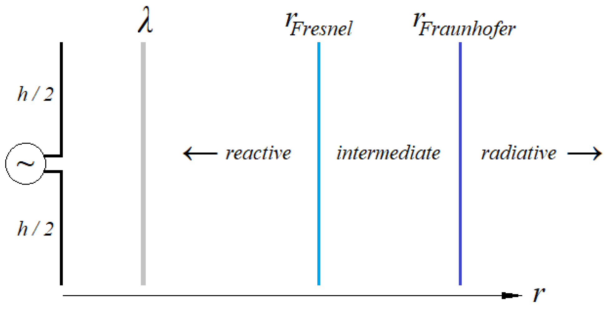
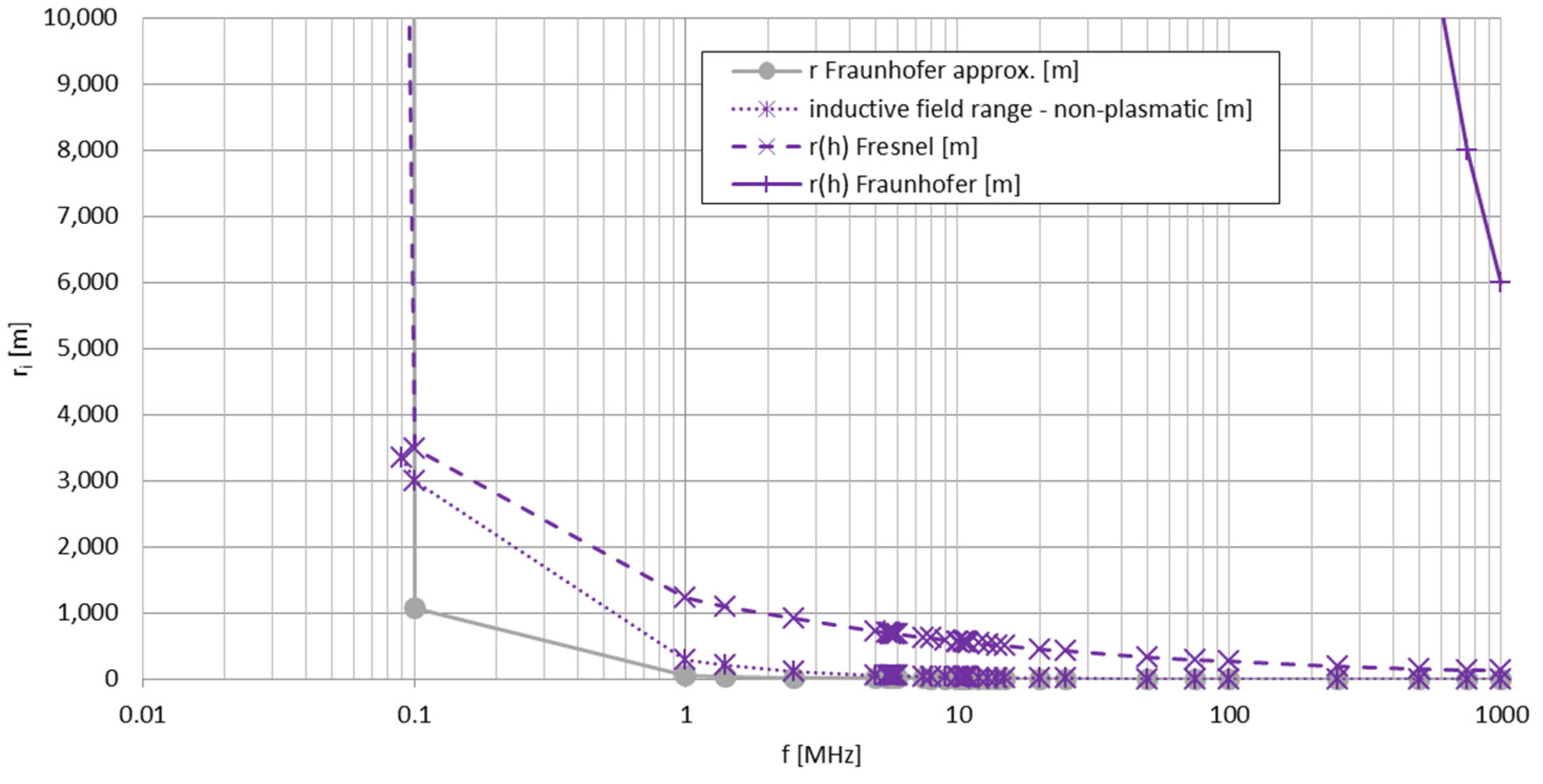
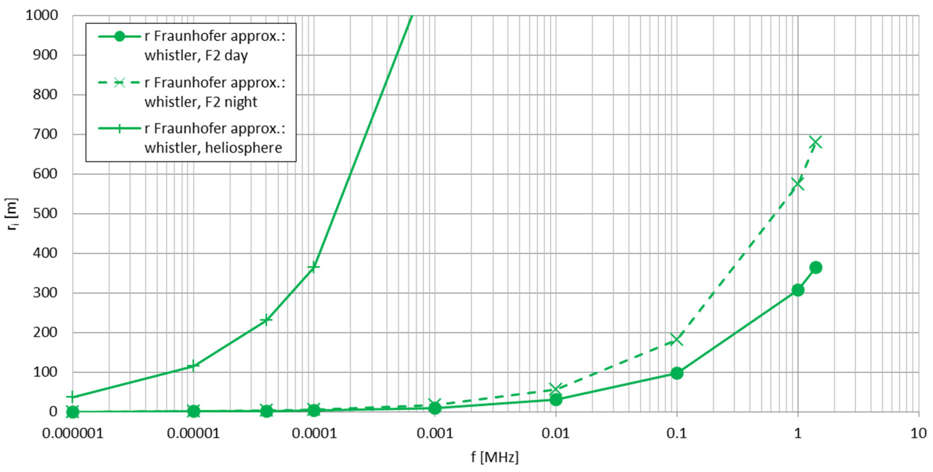
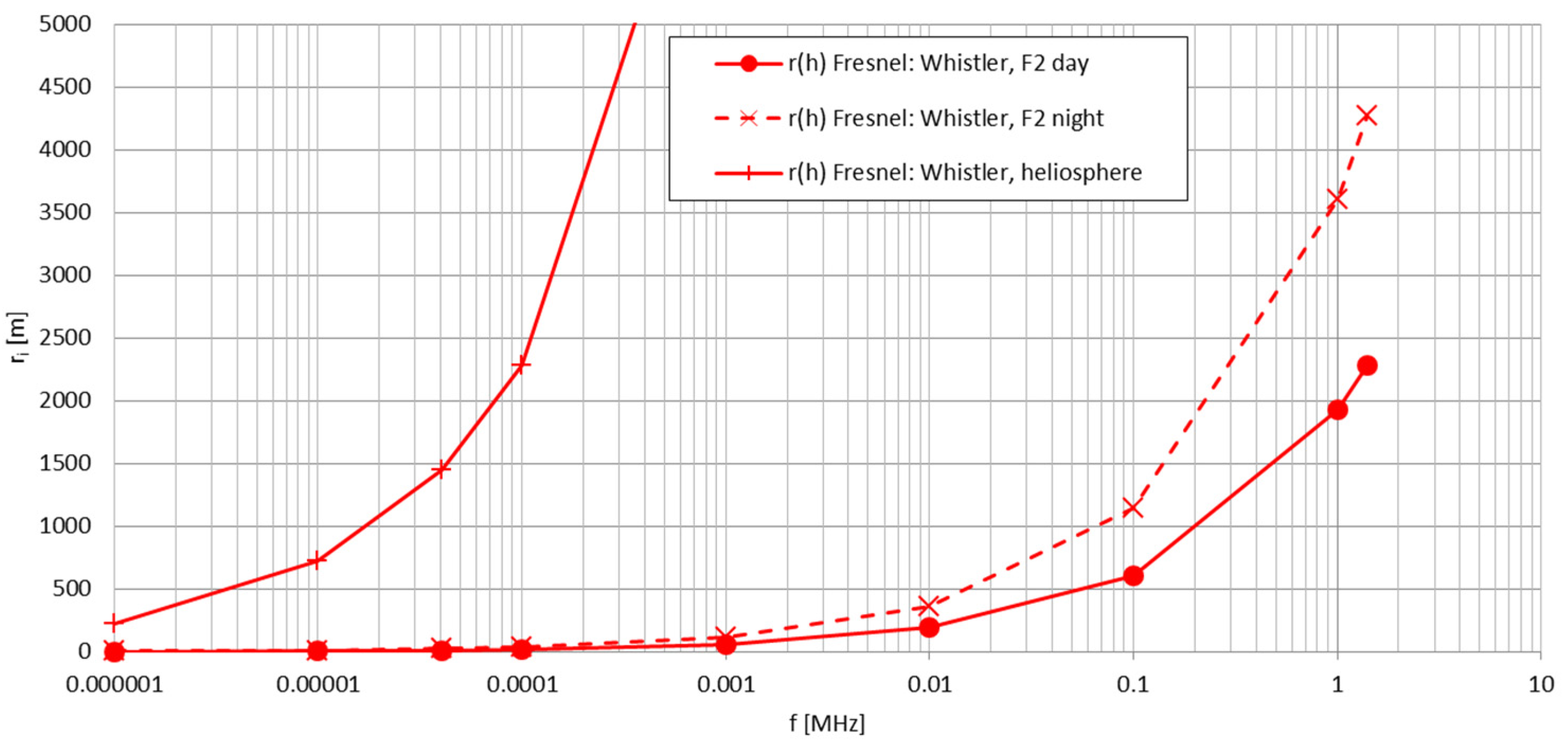
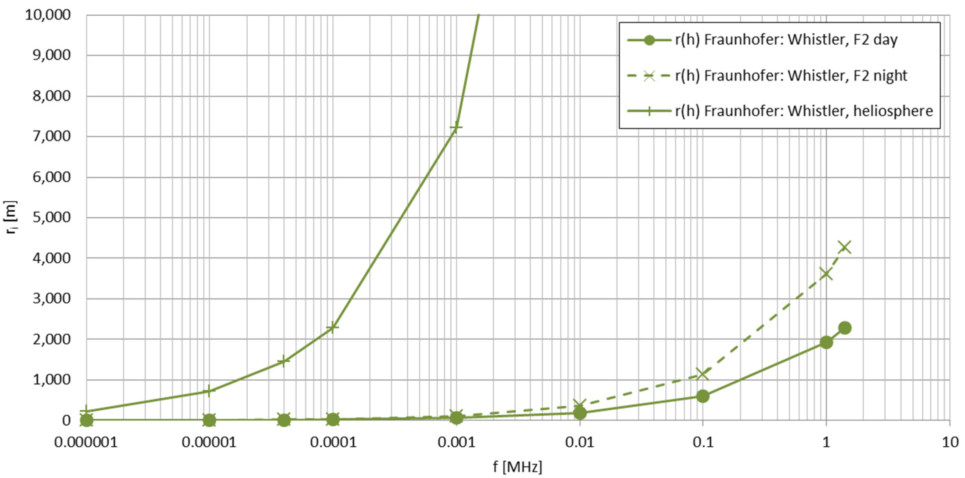
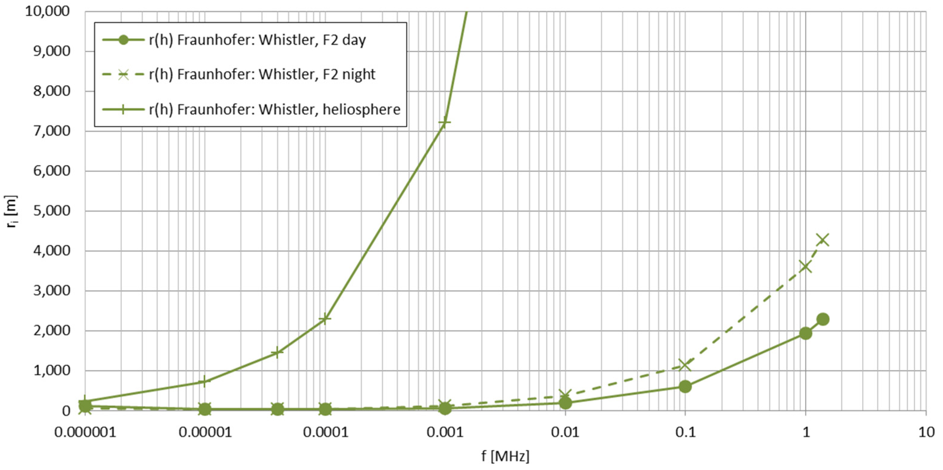
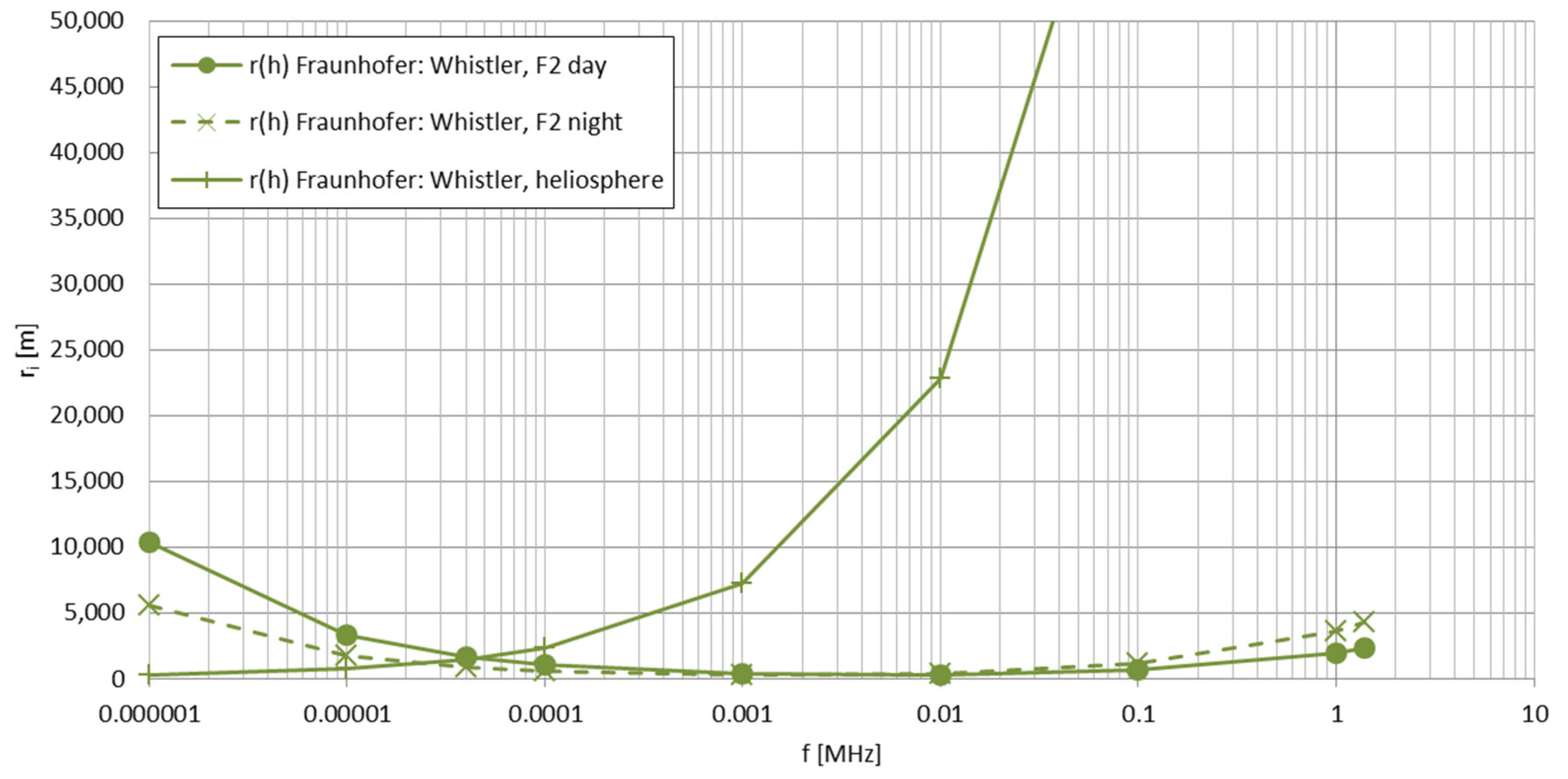
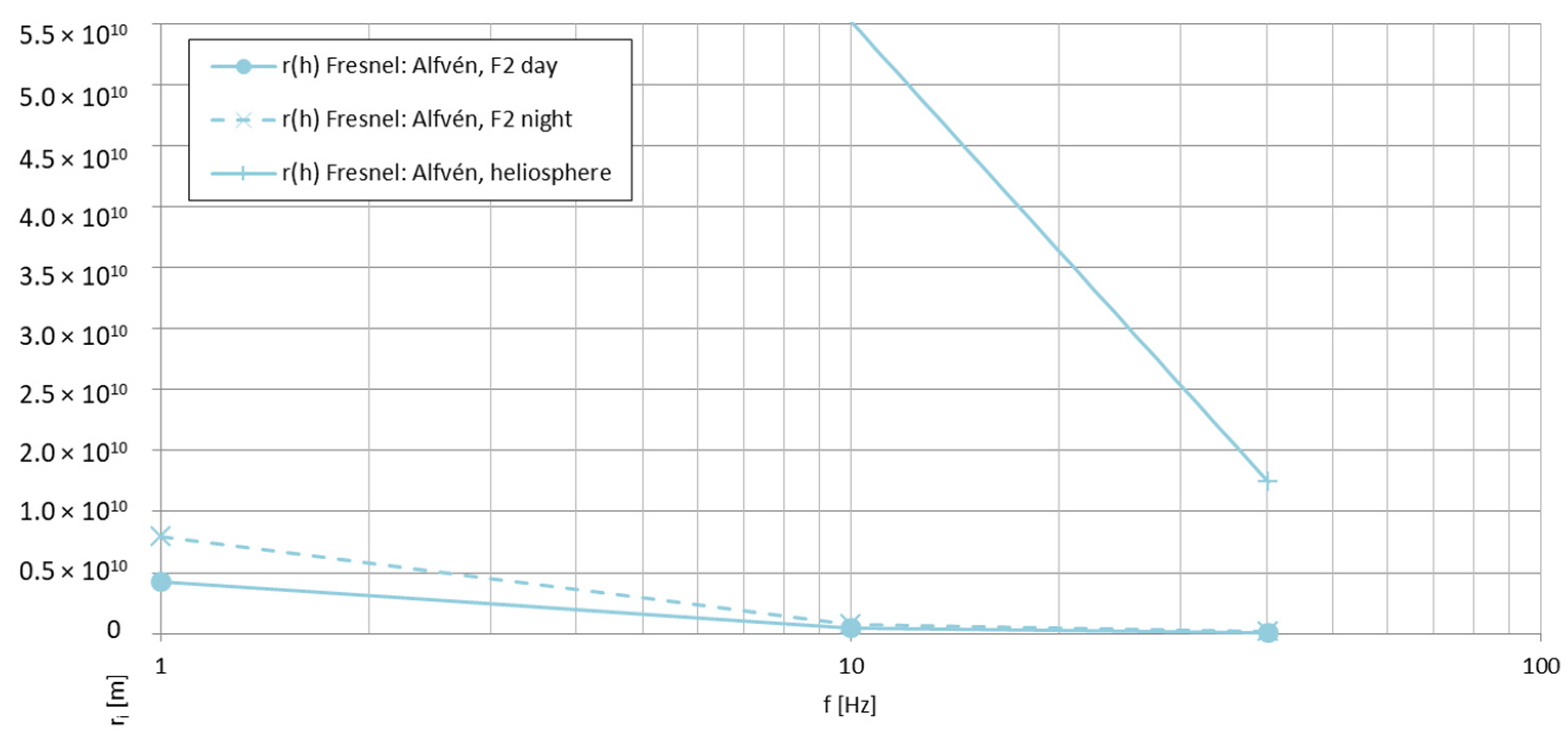
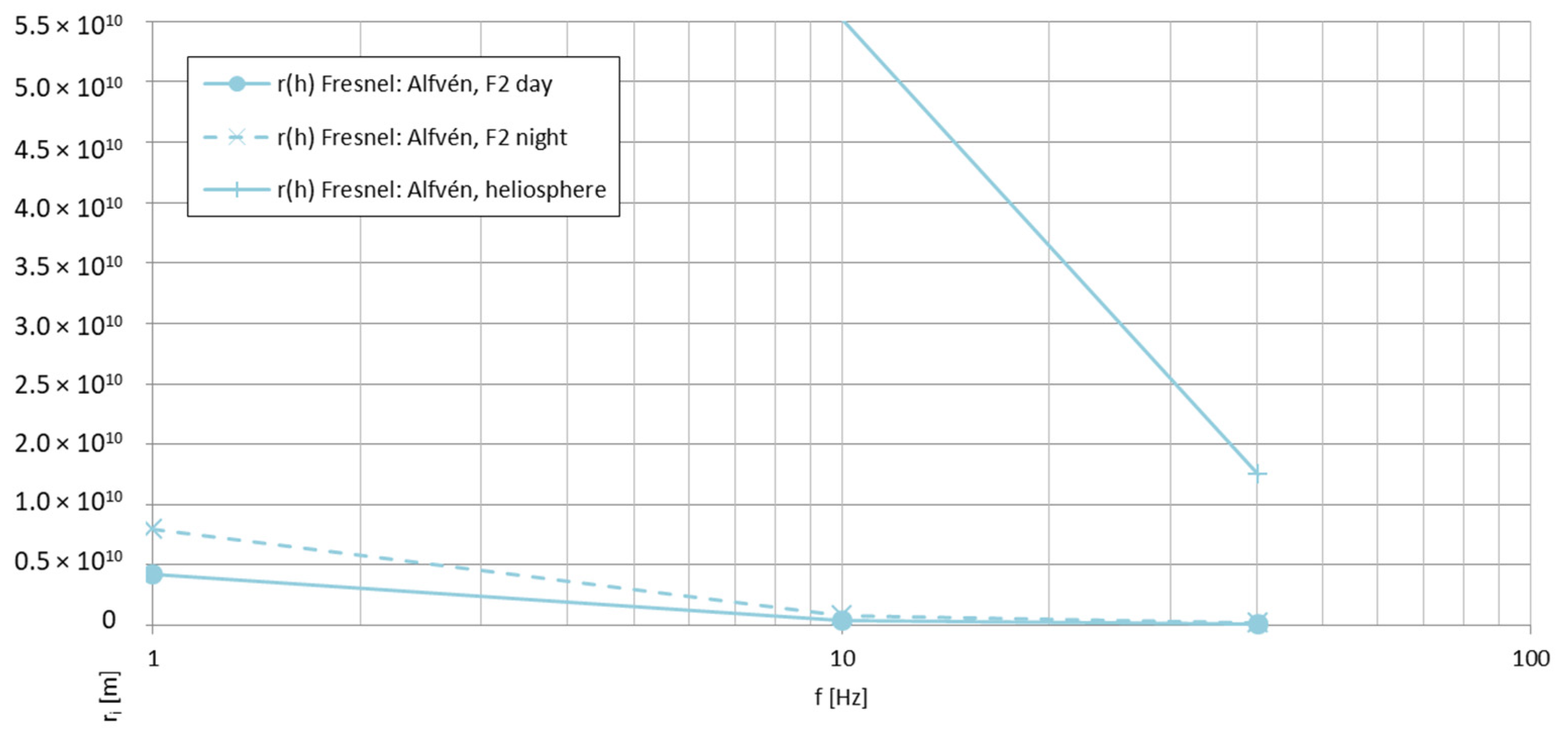
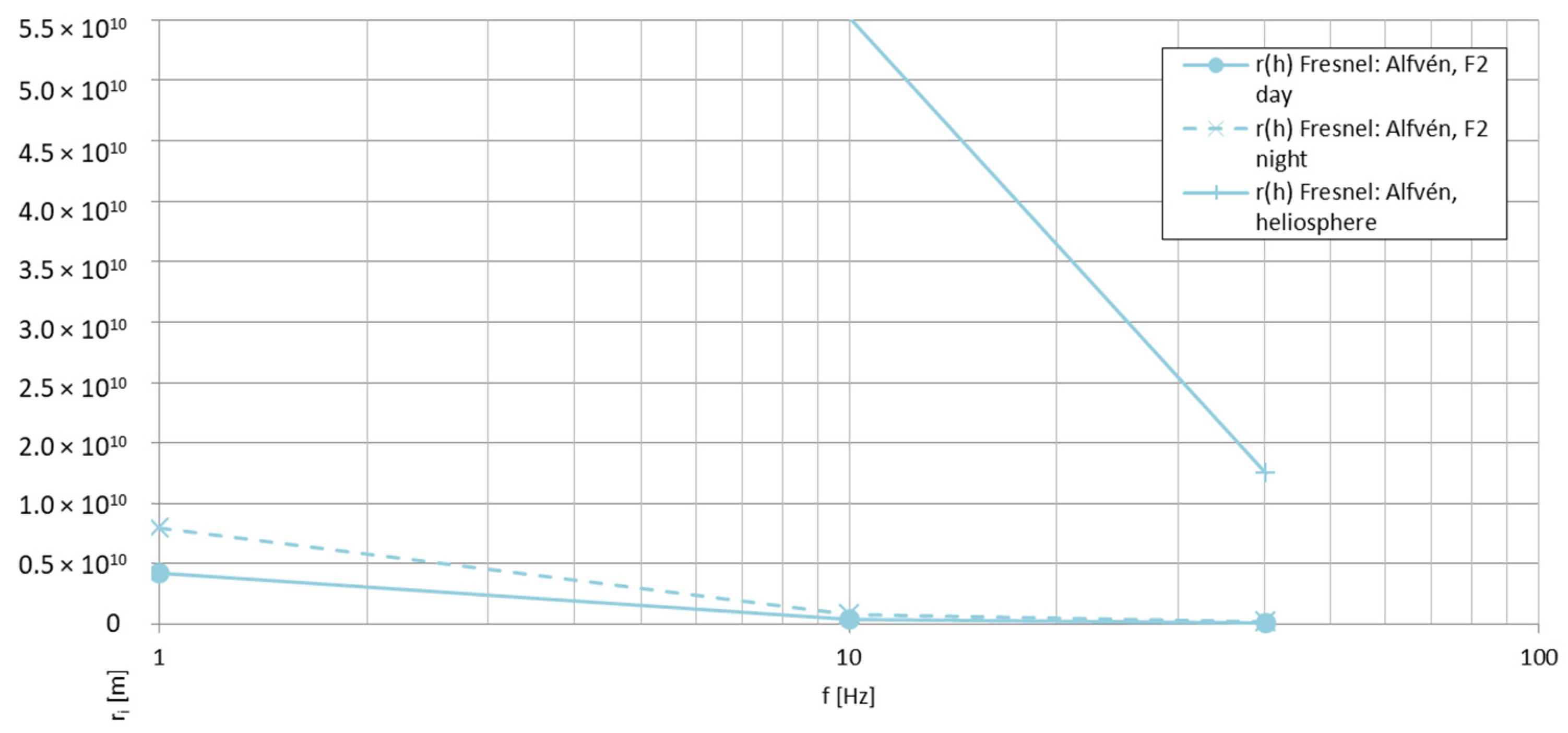
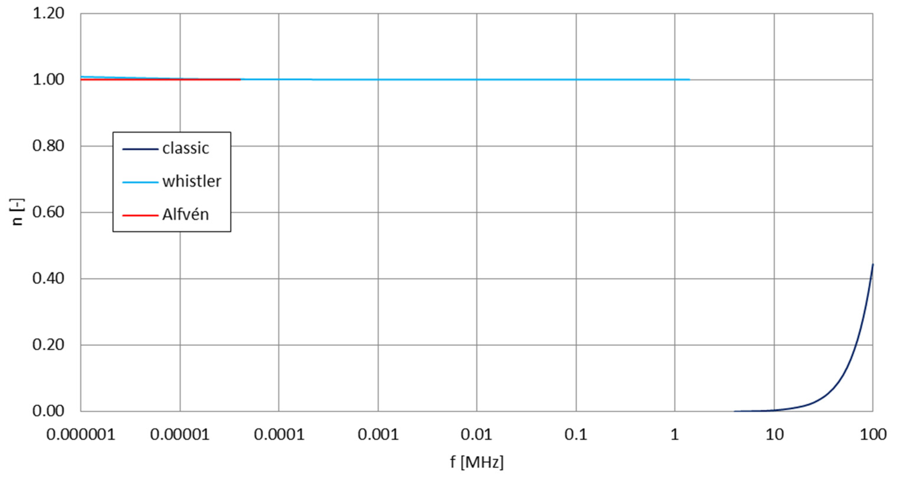
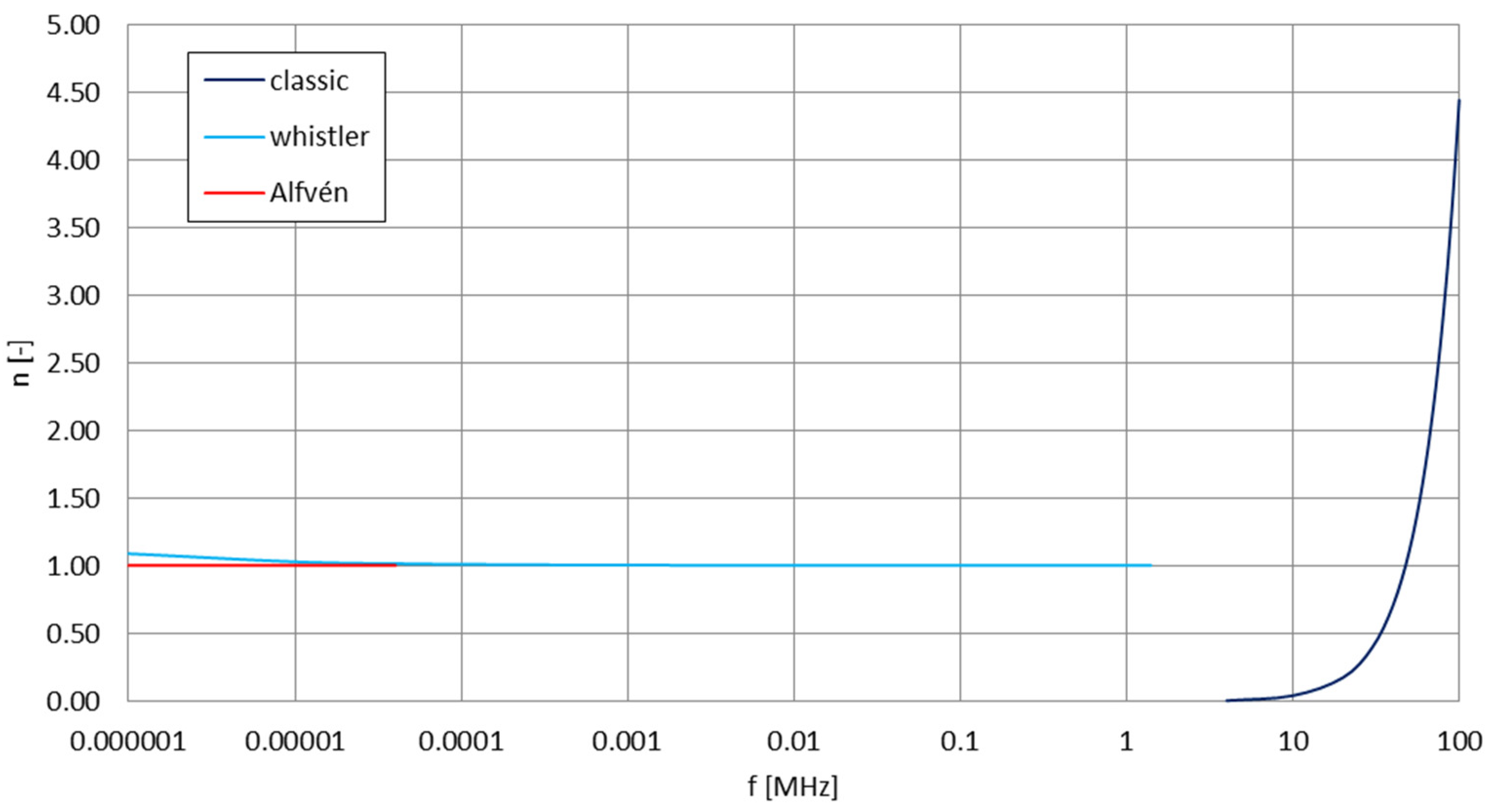
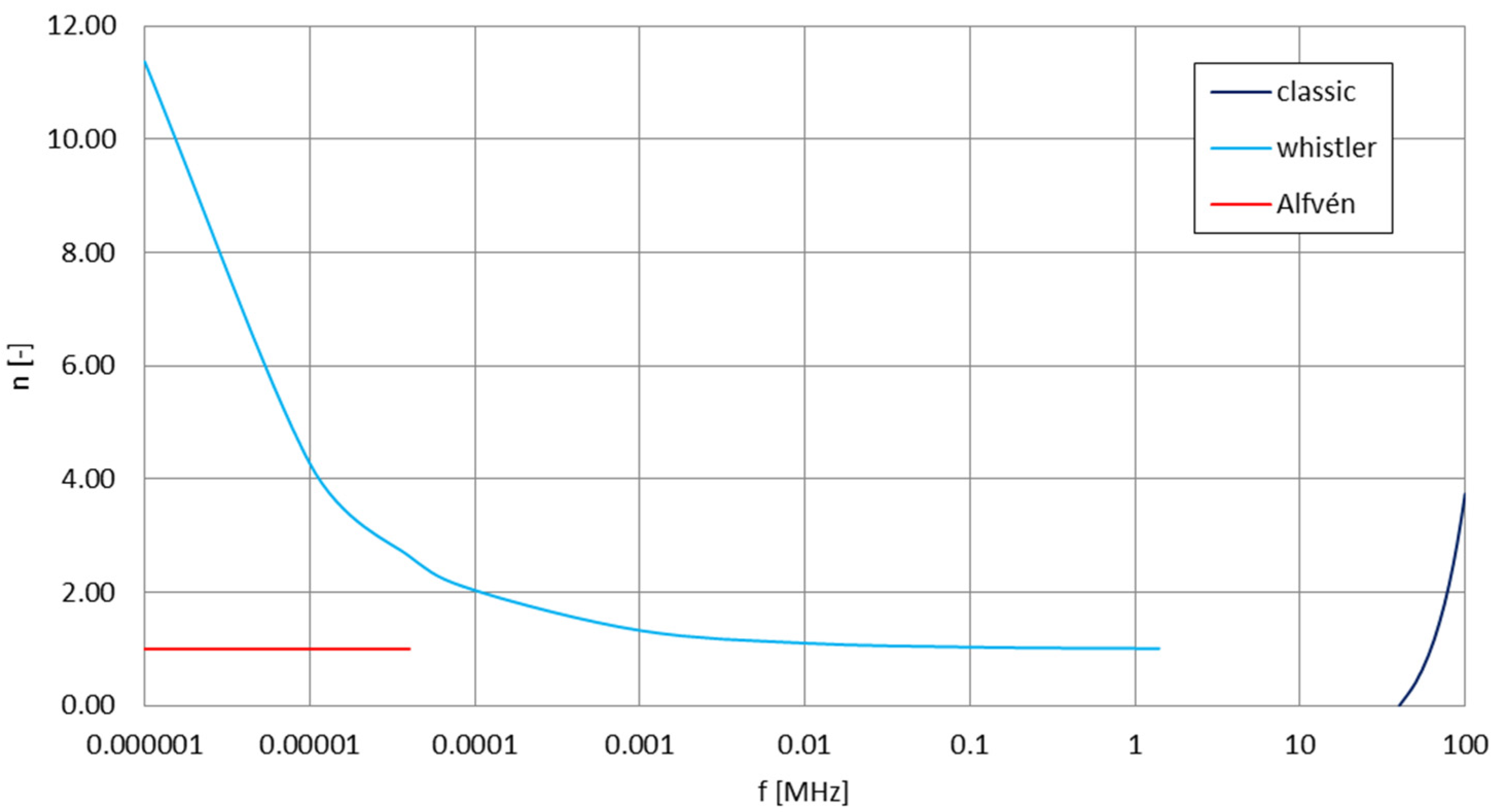
2. Evolution of the Radiation Zones

The zones of radiation around the antenna can be described as the ranges in which the energy radiated by the antenna is initially (close to the antenna surface) stored in the free space in a reactive form, then—with increasing distance to the antenna—the radio wave front is formed with its basic electric and magnetic field components; the energy takes the radiative form [36]. Figure 1 shows the basic schematic of the zones around a symmetrical dipole, indicating the Fresnel zone radius r_Fresnel, behind which the reactive form or emitted energy is dominant, and the Fraunhofer zone radius r_Fraunhofer, after which the radio wave front is fully shaped. Additionally, for a physical antenna dimension h smaller than the wavelength λ, the zone limited by the wavelength (deemed reactive) is also indicated [37].

The subsequent zone radiuses for the i-th λ can be defined as [37]:

$$r_{Fresnel}={\lambda }_i+{\displaystyle \frac{h}{2}}\sqrt[3]{{\displaystyle \frac{h}{2{\lambda }_i}}}$$

(1)

$$r_{Fraunhofer}={\lambda }_i+{\displaystyle \frac{2h^2}{{\lambda }_i}}$$

(2)

For the accurate mathematical formulations of the electric and magnetic field components on elevation θ, orientation ϕ and radial r directions from the antenna, the limiting distance which separates the reactive and radiative zones r_{Fraunhofer_approx.} can be defined as [38]:

$$r_{Fraunhofer\_approx.}={\left({\displaystyle \frac{4{\pi }^2}{{\lambda }_0^2}}-{\displaystyle \frac{e^2{n}_e}{m_e{\epsilon }_0{c}^2}}\right)}^{-{\displaystyle \frac{1}{2}}}$$

(3)

where λ₀ [m] is the free space wavelength, e is the electron electric charge (1.602 × 10⁻¹⁹ C), n_e [1/m³] is the electron concentration/density, m_e is the electron mass (9.109 × 10⁻³¹ kg), ε₀ is the free space electrical permittivity (8.854 × 10⁻¹² F/m) and c is the free space light velocity (300,000,000 m/s). For this formulation, the close zone of radiation (reactive) is located at distances r << r_{Fraunhofer_approx.}; for the intermediate zone: r ~ r_{Fraunhofer_approx.} and for the radiative zone: r >> r_{Fraunhofer_approx.}.

The i-th λ can be calculated as follows:

$${\lambda }_i={\displaystyle \frac{2\pi }{k_i}}$$

(4)

where k_i denoted the wavenumber for a given specific propagation mode. In this paper, three basic propagation modes for lower frequencies are considered—the whistler mode (k_W), i.e., for the frequencies below the local electron plasma frequency, approximated as 1400.564 kHz [35], the Alfvén mode (k_A), i.e., for the frequencies below the local ion gyromagnetic frequency, approximated as 40.215 Hz [35], and the wavenumber k_J calculated for the propagation conditions determined by the ionospheric cutoff frequency (denoted with subscript ‘classic’) for small current-element antenna [38].

For the whistler mode, as given by Bannister et al. [35], the wavenumber is equal to

$$k_W={\displaystyle \frac{1}{c}}\sqrt{{\displaystyle \frac{2\pi fe{n}_e}{B_0{\epsilon }_0}}}$$

(5)

where f [Hz] is the operating frequency, and B₀ [T] is the magnetic field induction parallel to the direction of propagation of the wave (perpendicular to the antenna axis).

For the Alfvén mode, after Bannister et al. [35], the wavenumber is formulated as follows:

$$k_A={\displaystyle \frac{2\pi f}{c}}\sqrt{{\displaystyle \frac{n_i{m}_i}{{\epsilon }_0}}}$$

(6)

where n_i [1/m³] is the ion concentration, equal to n_e, and m_i [kg] is the average ion mass, approximated as 3.17 × 10⁻²⁶ kg [35].

For the ‘classic’ ionospheric case (in which the wavefront enters the ionosphere and is subjected to absorption, refraction and reflection, solely depending on the frequency and n_e), the wavenumber is given by D. J. Bem [38] as follows:

$$k_J=\sqrt{{\displaystyle \frac{4{\pi }^2}{{\lambda }_0^2}}-{\displaystyle \frac{e^2{n}_e}{m_e{\epsilon }_0{c}^2}}}$$

(7)

similarly to the derivation of Formula (3).

The four radiuses of the subsequent radiation zones—inductive (for antenna length h [m] << λ₀), Fresnel, Fraunhofer and Fraunhofer classic—have been calculated for different exemplary electron concentrations: ionospheric F-layer in daylight conditions (1.4 × 10¹² m⁻³ [38]), ionospheric F-layer for night conditions (4 × 10¹¹ m⁻³ [38]) and heliospheric conditions, generalized as 10⁸ m⁻³ [39].

The three considered wavenumbers have been plotted in Figure 2, Figure 3 and Figure 4. Each electron concentration was employed for calculations for three different antenna lengths h: 1 m, 10 m and 100 m (antenna treated as a symmetrical dipole). It can be noticed that the orders of magnitude of the wavenumbers for the Alfvén cases differ significantly from those of the whistler and classic-ionospheric cases—this shall later cause the exclusion of some of the Alfvén cases from direct comparison with other cases due to their gargantuan sizes (when compared to the actual antenna aperture). For the heliospheric case, it can also be noticed that the classic-ionospheric function of k (Formula (7)) starts to overlap with the range for the whistler mode of k function (Formula (5))—it is therefore important to take into consideration the frequency range to which the given function is applicable and the final sizes of the resulting radiation zones’ radiuses, with the priority given to the smaller radius.

Figure 5, Figure 6 and Figure 7 present the radiation zones’ radiuses—Fraunhofer approximate (Formula (3)), Fresnel (Formula (1)), Fraunhofer (Formula (2)) and wavelengths for non-plasmatic cases (for λ << h)—for k_J and h = 1 m; Figure 8, Figure 9 and Figure 10: for k_J and h = 10 m and Figure 11, Figure 12 and Figure 13: for k_J and h = 100 m. It can be noticed that the Fraunhofer zone from Formula (2) expands significantly with the rise of dimensions of the antenna, while the approximate indication of the Fraunhofer zone (e.g., indicating the presence—or lack of presence—of certain fields components) remains more convergent to the inductive range (wavelength), with the Fresnel zone positioned as the largest in these orders of magnitude. These sets of functions and plots shall generally apply for low-MHz radio observations.

Figure 14 shows the approximate Fraunhofer radiation zones’ radiuses (3) for k_W and all considered n_e ranges (formula h-independent); Figure 15, Figure 16 and Figure 17: for the Fresnel zones’ radiuses (1) for k_W and all considered n_e ranges and h values; Figure 18, Figure 19 and Figure 20: for the Fraunhofer zones’ radiuses (2) for k_W and all considered n_e ranges and h values; Figure 21, Figure 22 and Figure 23: for the Fresnel zones’ radiuses (1) for k_A and all considered n_e ranges and h values (Fraunhofer zone radiuses for k_A were omitted due to large differences in the orders of magnitudes of their values in comparison to the values of the antenna aperture h).

It can be noticed that the approximate Fraunhofer zone radiuses (3) for heliospheric conditions remain many orders of magnitude higher for a given frequency than for the other electron-rich environments. Fraunhofer and Fresnel zones’ radiuses calculated using precise formulas show mainly dependence on the antenna length and its order of magnitude while maintaining the general (and similar to the previous case) relation between heliospheric and electron-rich cases. The Fraunhofer zone case for the largest (100 m) antenna length starts to exhibit changes/radius length increases for the lower frequencies (~kHz and lower), as the antenna length becomes more proportional to the signal’s wavelength.

3. Evolution of the Antenna Radiation Pattern’s Scalloping

The scalloping of the radiation (and, by the reciprocity theorem [40], reception) pattern of the antenna can be described as the length- or frequency-dependent appearance and relocation of minimums and maximums, redirecting the power transmitted by the antenna to certain directions or making the antenna more susceptible to signal reception at certain angles. If the exact solution [36] describing the number of maximums of the pattern—i.e., the lobes—is adapted to electron-rich conditions similarly to (3) and (7), the plasmatic solution for the number n_Plasma [-] of the scallops of the pattern can be defined as follows:

$$n_{Plasma}=⌈h\sqrt{{\displaystyle \frac{4}{{\lambda }^2}}-{\displaystyle \frac{e^2{n}_e}{m_e{\epsilon }_0{\pi }^2{c}^2}}}⌉$$

(8)

where the parentheses define the upper limit of the formula (i.e., value above 1 gives n_Plasma = 2, value above 2 gives n_Plasma = 3 etc.).

Figure 24 and Figure 25 present the number of the lobes (values of the formula within the parentheses) for the heliospheric environment (n_e = 10⁸ m⁻³) for all considered propagation cases (classic approach, whistler and Alfvén) and all considered antenna lengths h (1, 10 and 100 m); Figure 26, Figure 27 and Figure 28: for the ionospheric F-layer in daylight conditions (n_e = 1.4 × 10¹² m⁻³) and Figure 29, Figure 30, Figure 31 and Figure 32: ionospheric F-layer for night conditions (n_e = 4 × 10¹¹ m⁻³).

It can be noticed that for the heliospheric conditions, the MHz-range of the signal’s frequencies experiences an exponential rise in the number of pattern’s lobes, which increases significantly with the elongation of the antenna; for other (lower) frequencies, the pattern’s shape remains nearly constant. For the more electron-dense conditions (ionospheric F2 daytime), lower frequencies start to exhibit a strong exponential rise of the number of the pattern’s lobes, apart from the Alfvén case, which remains nearly constant. A similar mechanism, but lower in achieved values, can be noticed for the ionospheric F2 nighttime electron concentration conditions; it can be linked to the antenna length becoming more proportional to the signal’s wavelength for the lower frequencies and becoming rapidly oversized for the signal’s wavelength for the higher frequencies—the first mechanism can be noticed as ‘amplified’ by the increased electron density, and the latter mechanism appears as present globally.

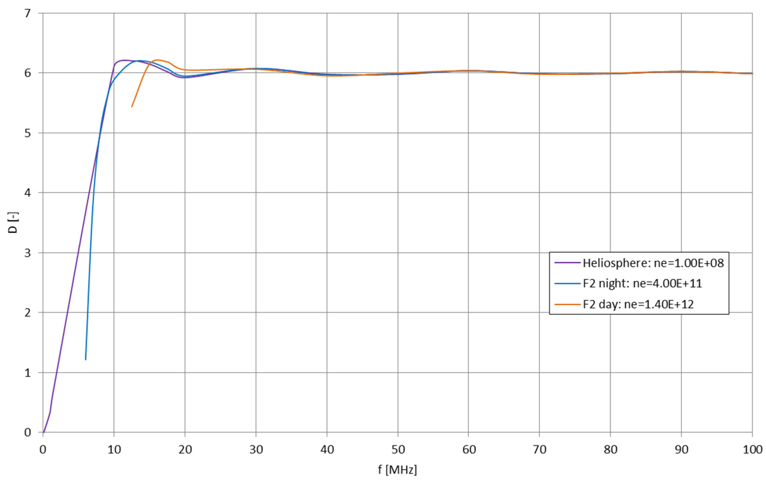
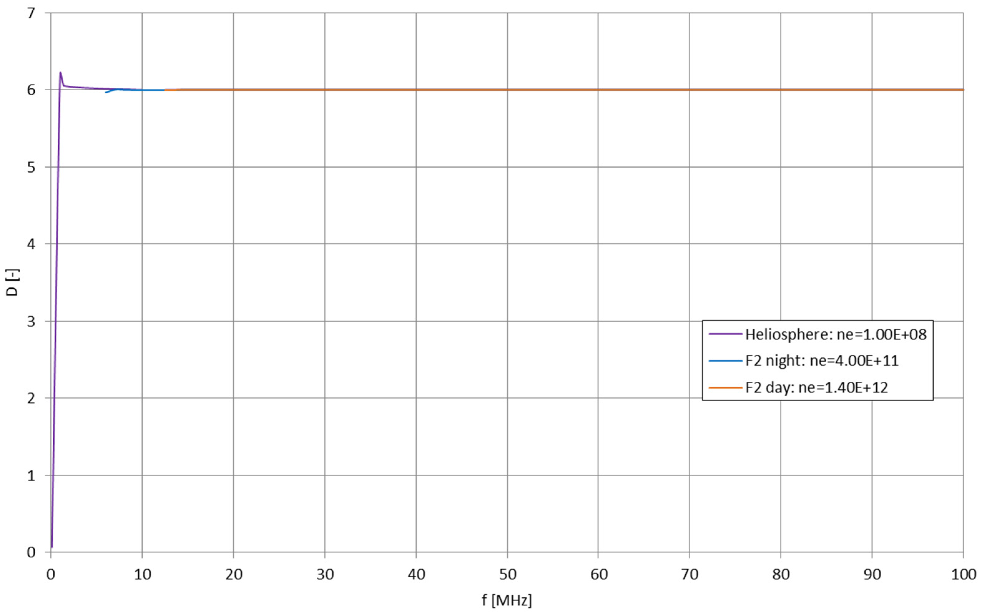
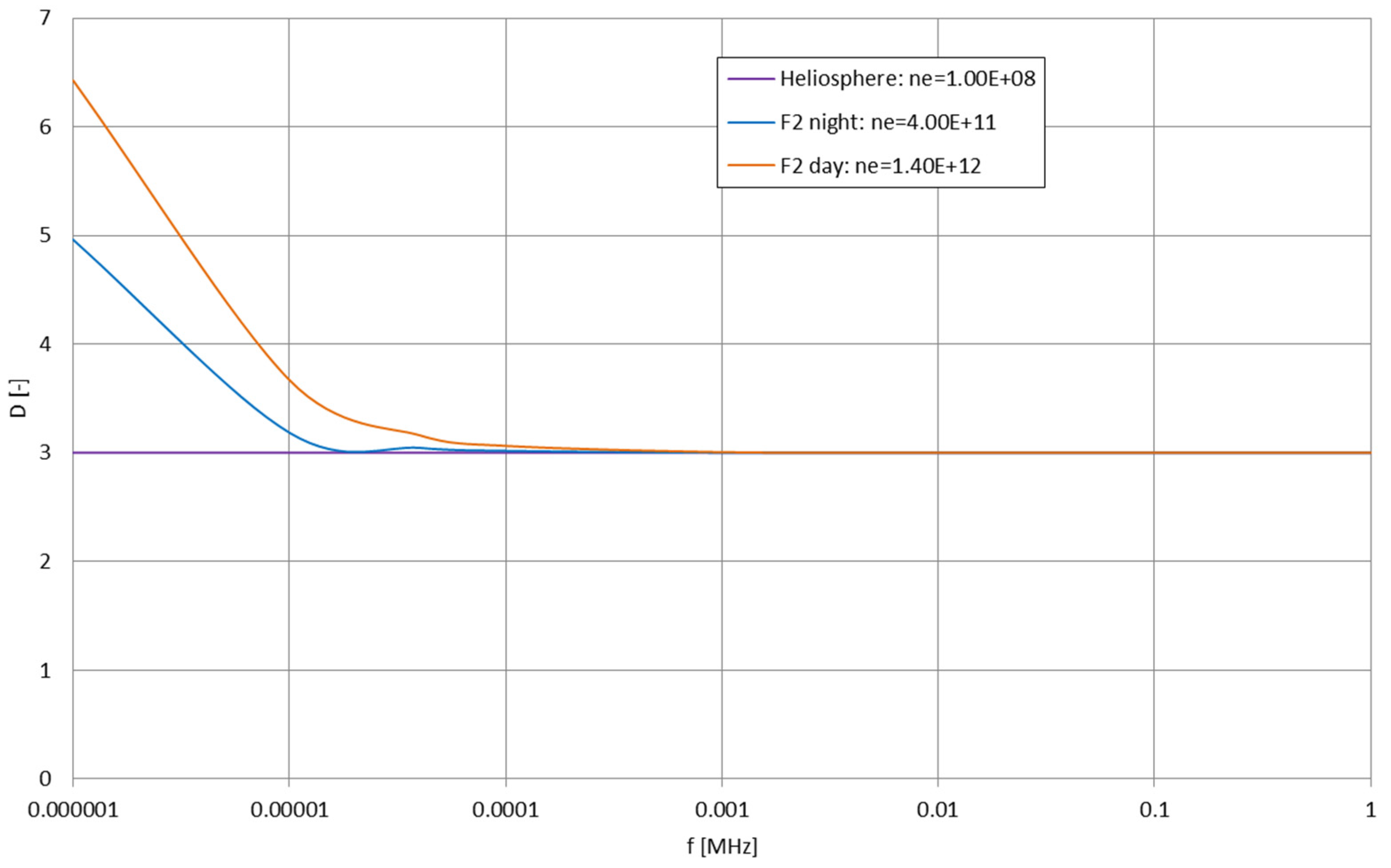
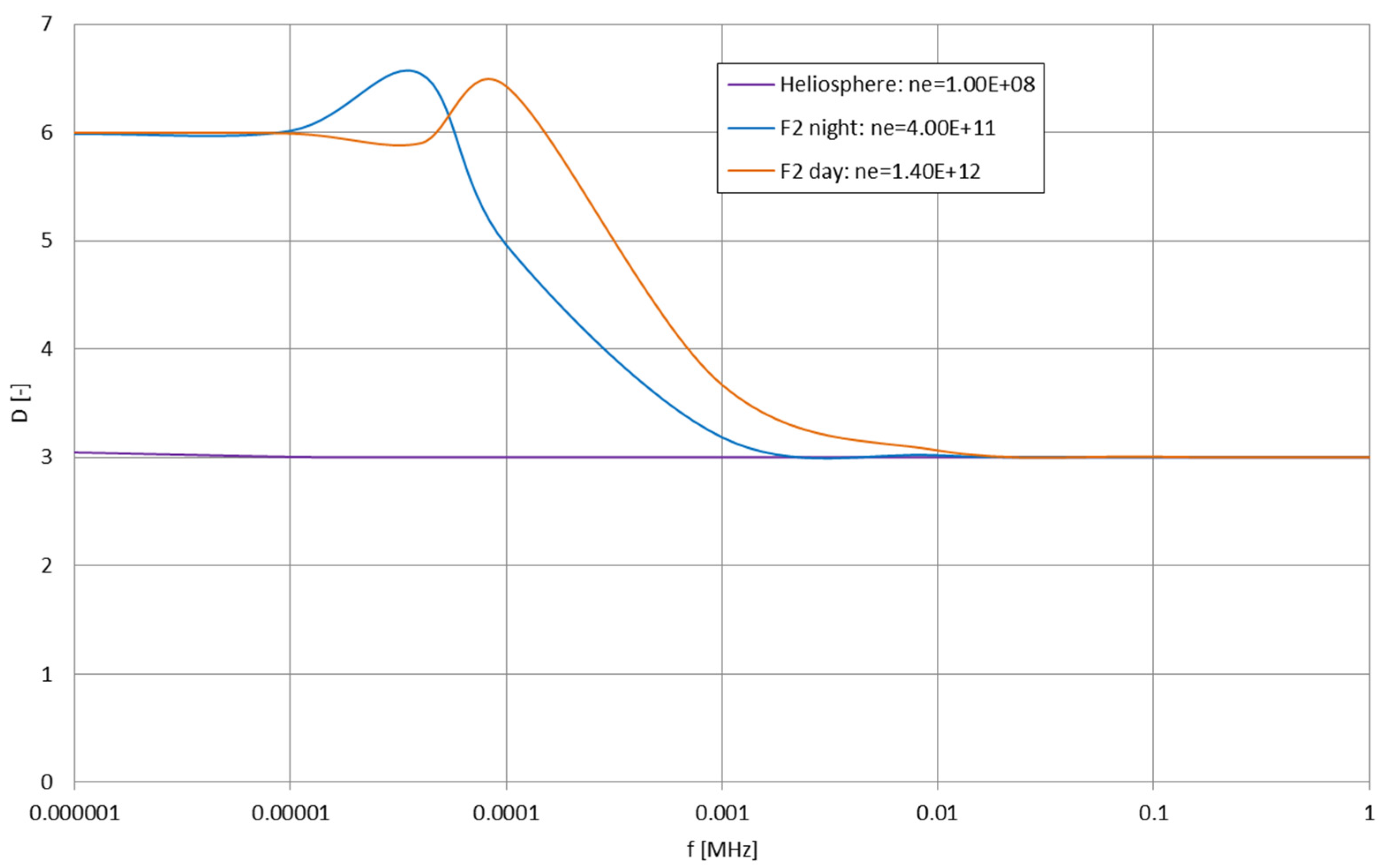
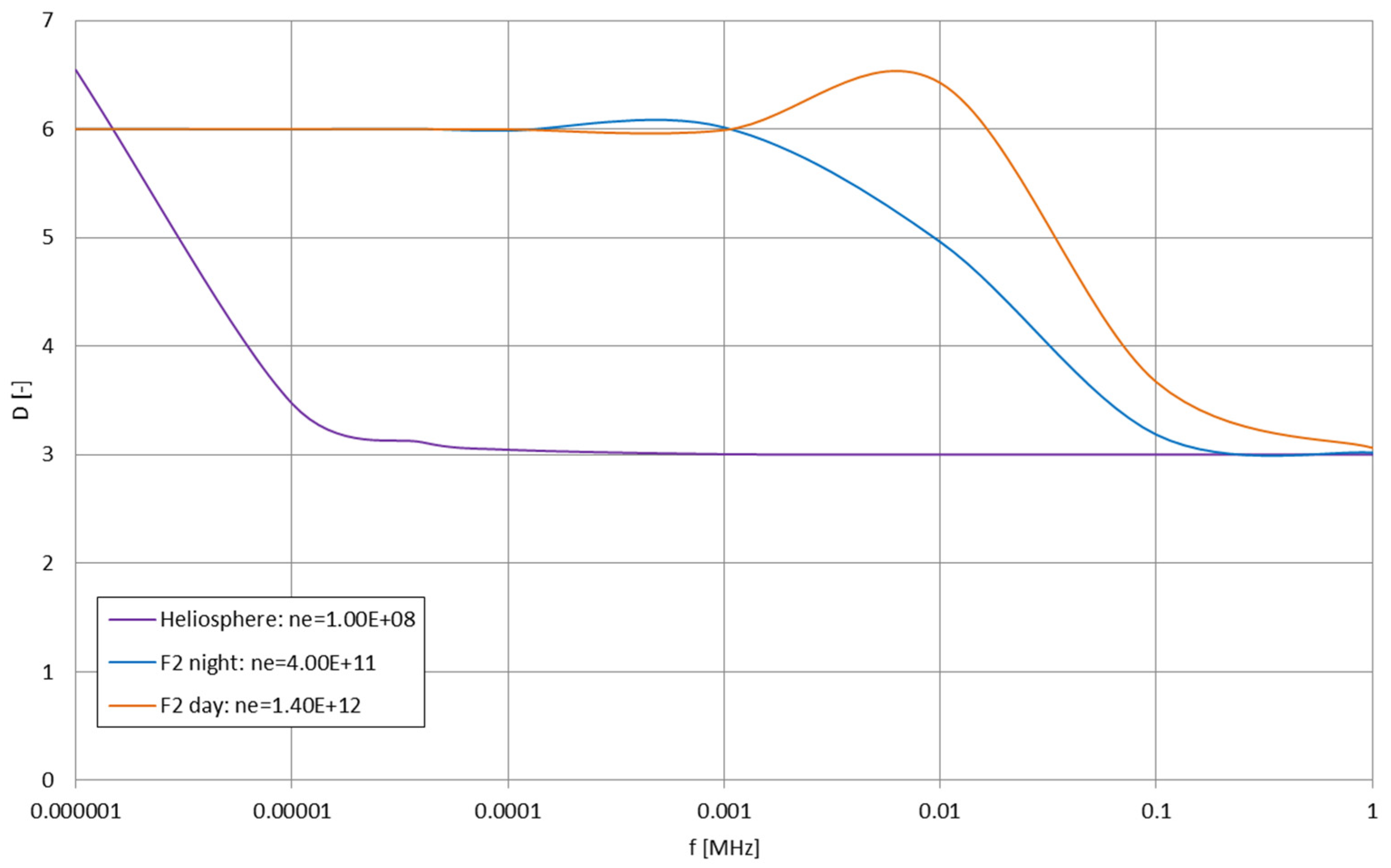
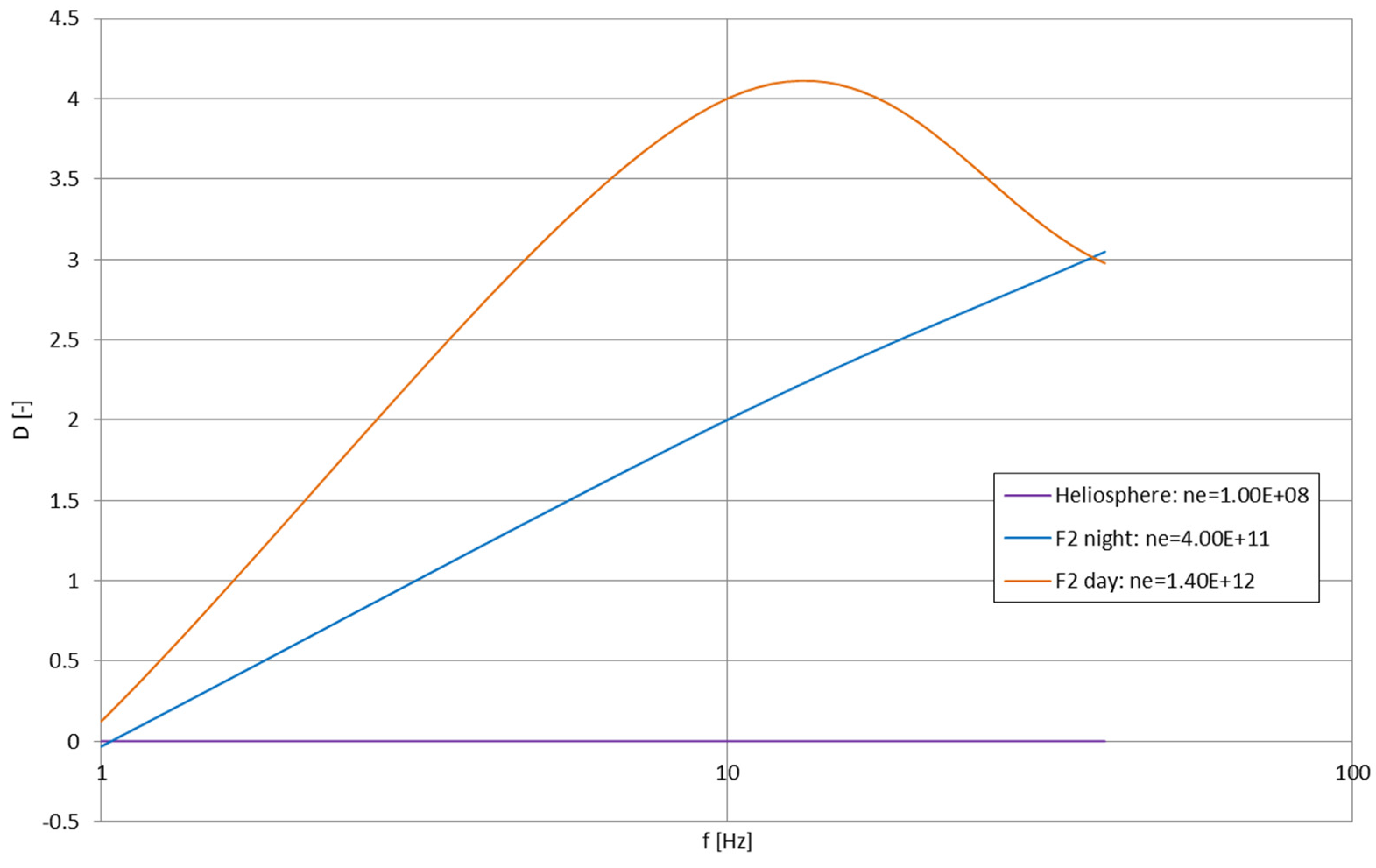
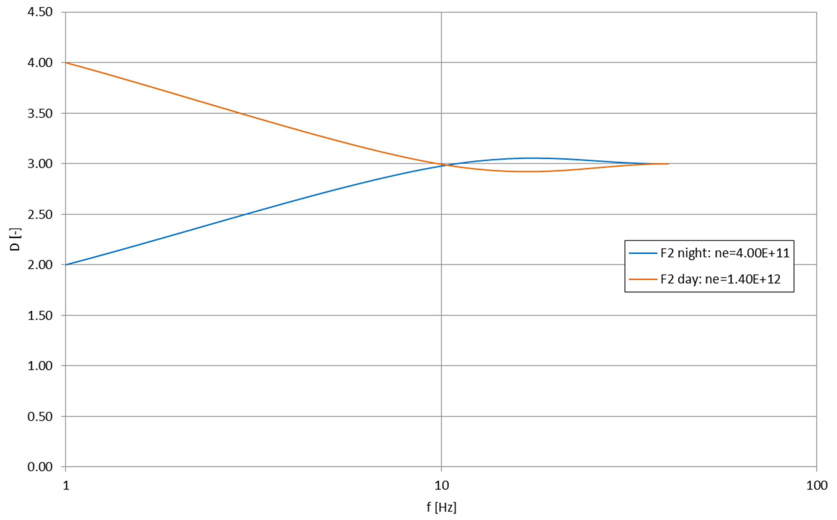
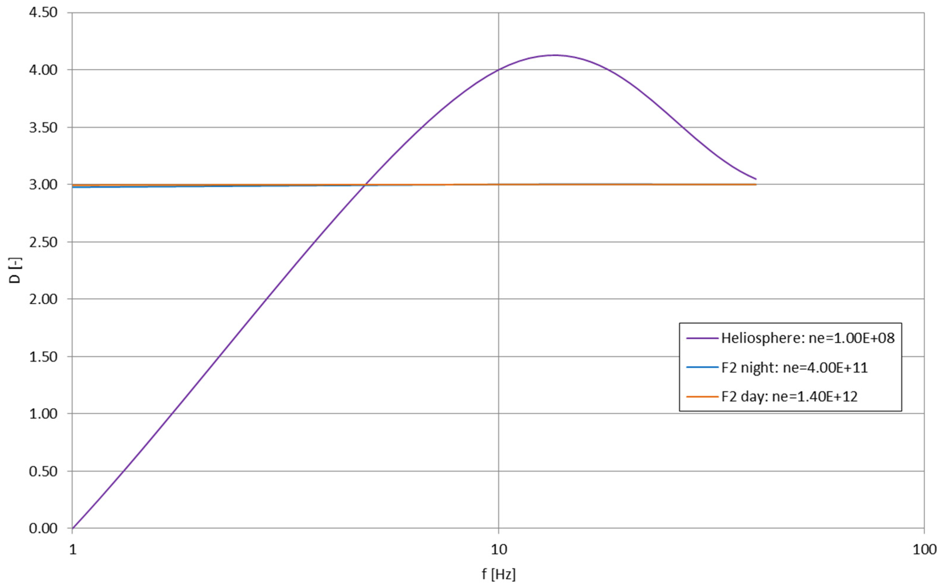
4. Evolution of the Antenna Radiation Pattern’s Directivity

The parameter of antenna’s directivity D [-] can be explained as the ability of the antenna to form a concentrated beam of radiated energy at a certain angular width—defined as the intensity of radiation at a given direction/angle divided by the averaged radiation intensity over the entire radiation pattern (2π). Together with the antenna’s efficiency η_A [-] (which depends on the radiation resistance of the antenna and its loss resistance), it gives the antenna’s gain G [-]: G = Dη_A [40]; the antenna’s gain is therefore directly proportional to the directivity, with the antenna’s efficiency heavily dependent on the radiation losses in the actual spacecraft application (the radiation resistance for a dipole as a function of length-to-wavelength ratio remains well known [40]).

The directivity formula can be expressed as [36] follows:

$$D_i=2{\left({\displaystyle \frac{1}{3}}-{\displaystyle \frac{\cos \left(2h{k}_i\right)}{{\left(2h{k}_i\right)}^2}}+{\displaystyle \frac{\sin \left(2h{k}_i\right)}{{\left(2h{k}_i\right)}^3}}\right)}^{-1}$$

(9)

with k_i defined for each case (ionospheric, whistler or Alfvén) using Formulas (5), (6) and (7). Figure 33, Figure 34 and Figure 35 present the directivity calculated for the classic (7) case for different previously considered electron concentrations and antenna lengths h = 1, 10 and 100 m; similarly, Figure 36, Figure 37 and Figure 38 employ the whistler wavenumber (5) and Figure 39, Figure 40 and Figure 41: the Alfvén wavenumber (6).

For the classic-ionospheric cases, the longer the antenna, the more constant the directivity, reaching a value of 6 for high-MHz frequencies; for the kHz-and-lower frequency range, the directivity reaches values below 1, which indicates a lack of a well-formed separate lobes in the radiation pattern (as in the Figures in the previous paragraph). For the whistler propagation mode, the general behavior of the directivity changes moves upward with the frequency values with the increase in the antenna length; both ionospheric conditions show two maximums at about 6.5, while the heliospheric case starts to give larger values at the largest considered antenna length of 100 m. For the Alfvén propagation mode and frequency range, in Figure 40, the heliospheric conditions produced numerical errors in Formula (9) and were not included in the final plot; the smaller the antenna, the more susceptible it appears to higher electron concentrations, with the largest considered antenna of 100 m showing high variability to the lowest (heliospheric) electron concentration. For all the Alfvén cases, the maximum directivity value reached 4.1.

5. Radiation Pattern Transformation Coefficient from the Air/Vacuum to Plasmatic Conditions

The experimental verification of the shape of the antenna radiation/reception pattern, which always incorporates the actual mechanical configuration of the antenna and the antenna mounting (e.g., on a spacecraft), is mainly possible either for the terrestrial atmospheric conditions or close-to-vacuum conditions (if additional heat transfer, typical for space environment, is required to be re-created for other components). Analytical solutions for the radiation/reception pattern of a given antenna submerged in the plasma of given parameters have been developed—e.g., the radiation pattern by Bannister et al. for the i-th wavenumber k [35]:

$$f_P\left(\theta \right)={\displaystyle \frac{\sin \theta }{1-\cos \theta }}\sin \left[{\displaystyle \frac{1}{2}}{k}_{i}h\left(1-\cos \theta \right)\right]$$

(10)

where θ [rad] is the angle between the symmetry plane of the antenna (considered as a symmetrical dipole of the total length h [m]) and the main axis of the antenna. This radiation pattern shows the common (for large plasmatic antennas) property of radiating the energy over a direction close to the main axis of the antenna, which manifests itself stronger with the increasing length of the antenna [24,34,35] and remains totally inconsistent with the shape of the pattern/antenna behavior in non-plasmatic conditions [23]. This property remains of interest not solely for the antenna testing purposes and the actual in-plasma transmitting antenna applications, but also for the receiving antennas submerged in plasmas, which—as their reception pattern evolves in relation to the plasma around them—may change in a way which shall exclude some of the directions to the antenna from receiving any signal; this shall remain useful for the accurate description of, e.g., the incoming directions and actual signal strengths of the Auroral Kilometric Radiation.

A method based on a simple transformation of the analytical definitions of the radiation pattern’s shape from the air/vacuum conditions to the plasmatic conditions—with the assumption that this approach remains valid for the experimentally defined pattern shapes—for a given θ angle value can be defined as follows:

$$T_{\theta =const.}\left(f_{A real}\left(\theta \right)\to f_{P real}\left(\theta \right)\right) : f_{P real}=f_{A real}\left(\theta \right){\displaystyle \frac{f_P\left(\theta \right)}{f_A\left(\theta \right)}}$$

(11)

where f_i(θ) are the functions of the antenna radiation patterns and the subscripts P, A and real describe air/vacuum, plasmatic and real conditions, subsequently. The ratio of the plasmatic-to-air/vacuum radiation pattern functions requires an additional division of each f_i(θ) function by the maximum value reached by it, in order to make the subsequent cases comparable in values (this would, however, erase the accurate information on the directivity). Naturally, for this transformation, the value of f_A(θ) must not reach zero (may reach a real value of ε → 0) and remains valid for the condition below (otherwise it is a tautology):

$${\int }_{\epsilon \to 0}^{{\displaystyle \frac{\pi }{2}}-\epsilon }{f}_A\left(\theta \right)d\theta \ne {\int }_{\epsilon \to 0}^{{\displaystyle \frac{\pi }{2}}-\epsilon }{f}_P\left(\theta \right)d\theta$$

(12)

For the actual space-applied conditions and measured different radio signals mentioned in paragraph 1, the precise direction of the incoming signal is not always known, and the evolution of the antenna radiation/reception pattern for different plasmatic conditions shall introduce even more variables to its definition. If a two-dimensional frequency spectrum is obtained from such antenna, and basic plasma parameters are accessible (as described in paragraph 2), the ratio from the Formula (11) can be expanded to form a general frequency- and angle-dependent coefficient w(θ,f), which includes the plasmatic radiation pattern (10) and air/vacuum radiation pattern for short linear antenna [36]; the differences between the air/vacuum and plasmatic antenna radiation patterns are defined in the space around the antenna wire and over the entire possible range of θ (with the integration-facilitating assumption that the antenna is a symmetrical dipole of the total length h):

$$w\left(\theta ,f\right)=4\pi {\int }_{\epsilon \to 0}^{{\displaystyle \frac{\pi }{2}}-\epsilon }{\displaystyle \frac{f_P\left(\theta \right)}{{\mathrm{m}\mathrm{a}\mathrm{x}[f}_P\left(\theta \right)]}}{\left({\displaystyle \frac{f_A\left(\theta \right)}{\max \left[f_A\left(\theta \right)\right]}}\right)}^{-1}d\theta =4\pi {\int }_{\epsilon \to 0}^{{\displaystyle \frac{\pi }{2}}-\epsilon }{\displaystyle \frac{\sin \left[\frac{1}{2}{k}_{i}h\left(1-\cos \theta \right)\right]}{\sin \theta \left(1-\cos \theta \right){\cos }^2\left(\frac{2\pi fh}{c}\cos \theta \right)}}{\displaystyle \frac{\max \left[f_A\left(\theta \right)\right]}{{\mathrm{m}\mathrm{a}\mathrm{x}[f}_P\left(\theta \right)]}}d\theta$$

(13)

An approximate solution can be computed as follows:

$$w\left(\theta ,f\right)\approx {\sum }_{i=1}^n{\displaystyle \frac{1}{2}}{\theta }_i{\displaystyle \frac{\max \left[f_A\left(\theta \right)\right]}{{\mathrm{m}\mathrm{a}\mathrm{x}[f}_P\left(\theta \right)]}}\left({\displaystyle \frac{\sin \left[\frac{1}{2}{k}_{i}h\left(1-\cos {\theta }_i\right)\right]}{\sin {\theta }_i\left(1-\cos {\theta }_i\right){\cos }^2\left(\frac{2\pi fh}{c}\cos {\theta }_i\right)}}+{\displaystyle \frac{\sin \left[\frac{1}{2}{k}_{i}h\left(1-\cos {\theta }_{i-1}\right)\right]}{\sin {\theta }_{i-1}\left(1-\cos {\theta }_{i-1}\right){\cos }^2\left(\frac{2\pi fh}{c}\cos {\theta }_{i-1}\right)}}\right)$$

(14)

As the wavenumbers k_i may incorporate the B₀ magnetic field compound, it is necessary to approximate this compound in a way which reflects the structure and direction of the magnetic field around the antenna. For a case where the magnetic field induction remains constant along the Z axis of the antenna, the B₀ parameter can be formed as follows:

$$B_0={\int }_0^{2\pi }{B}_{0 max.}\left|\sin \varphi \right| d\varphi =4B_{0 max.}$$

(15)

where ϕ [rad] is the angle laying in the plane parallel to the plane of symmetry of the dipole. If B₀ remains not constant along the antenna wire and has a known distribution function with the maximum value of B_{0 max.} and the argument of z, the formula is presented as follows:

$$B_0\left(z\right)={\int }_0^{{\displaystyle \frac{h}{2}}}{\int }_0^{2\pi }{B}_{0 max.}\left(z\right)\left|\sin \varphi \right| d\varphi dz=4{\int }_0^{{\displaystyle \frac{h}{2}}}{B}_{0 max.}\left(z\right) dz$$

(16)

Figure 42, Figure 43, Figure 44 and Figure 45 present the w(f) coefficient (after the integration over θ) calculated for a wide frequency range for different electron concentrations (as in the previous paragraphs) and subsequent antenna lengths: 1, 10 and 100 m. As the Formulas (13) and (14) incorporate the Formula (10), which is essentially valid for the whistler propagation mode frequency range, the maximum frequency in these figures does not exceed the value of 1.4 MHz—the calculation beyond this limit would be possible after the clarification of the accuracy of Formula (10) above this frequency.

For the smaller antenna lengths, the calculated coefficients demonstrate a nearly constant behavior, slightly rising for the higher frequencies for denser electron conditions (F2 layer in daylight) and slightly decreasing for the less dense electron conditions (heliospheric). For the largest considered antenna length of 100 m, the coefficient shows multiple significant changes in values for the more electron-dense conditions, which demonstrate the differences between the antenna radiation patterns for air/vacuum and plasmatic cases. As the coefficient is meant to bring the air/vacuum case in value to the plasmatic case, it reacts on the appearance of the lobes in the pattern, including any sign switching of the function, which—from a mathematical point of view—may appear.

6. Discussion

The presented evolutions of the basic antenna parameters describing its abilities to radiate or receive electromagnetic energy clearly shows the dependence on the electrical conditions or the surrounding space—as presented, these conditions do not only influence the impedance of the antenna (as shown in various previous research from the past decades), but its functioning in space as energy radiators or energy receivers. It is important from two major aspects—the aspect of the spacecraft and antenna design and the aspect of interpreting and using data from the existing spacecraft and its instrumentation.

The design aspect concentrates mainly on the allocation of the antennas in the proximity of the spacecraft in a way which would prevent the measurements of the plasma influenced directly by the spacecraft (appearing around the structure of the spacecraft—unless this is a specific requirement for the mission). This direct influence can be linked to the presence of the conductive structures (booms/beams, solar panels, spacecraft frames etc.) within the Fresnel or the Fraunhofer zones around the antenna.

The zones’ radiuses, calculated using different formulas in paragraph 2, clearly show the evolution with the changing plasma parameters—they remain highly sensitive to different electron concentrations n_e. For the smaller antennas (~10⁰ m in length), all the zones’ radiuses are relatively condensed; it is therefore not difficult to include in the instrumentation mechanical design requirements the requirement of placing larger structures beyond the Fraunhofer zone radius (up to a maximum frequency of interest). With the increasing length of the antenna (~10¹–10² m), the accurate (formula-based) Fraunhofer zone becomes too large to be easily included as a dimensional requirement; therefore, the Fresnel zone radiuses—or the approximate formula for the Fraunhofer zone radius, derived from the characteristics of the EM fields around the antenna—can be considered.

For a case where the spacecraft is already designed, built and in operation, these radiuses can be used as indicators whether it would be beneficial to verify the actual radiation/reception pattern of the antenna in a way which includes the spacecraft mechanical elements as passive antenna reflectors. This is especially important for the reception of the radio signals propagating in the whistler and Alfvén-wave modes, which have significantly larger Fraunhofer and Fresnel zones’ radiuses, ranging to the size of an entire satellite constellation.

The rise of the electron concentration n_e also influences the scalloping of the antenna radiation/reception pattern; for the highest considered concentrations, proportional to those in the ionospheric F2 layer in daylight conditions (photoionization etc.), the appearance of the separate pattern lobes (maximums and minimums) is present for both the whistler propagation mode at lower frequencies (~kHz and lower) and for the high MHz frequencies. The increase in scalloping is also directly related to the proportion of the incoming signal’s wavelength to the antenna’s length, which manifests itself simultaneously with the influence of the growing n_e.

Sufficiently prominent lobes shall elevate the parameter of directivity, which can be used—together with the antenna’s efficiency parameter—to define the antenna gain, or simply to describe the effectiveness of the antenna radiation of reception at a given frequency in a plasma of given parameters. The behaviors of the directivity are significantly different for every propagation mode case and every considered n_e value—this requires a careful approach for a precise set of measurement requirements, e.g., frequency range and expected plasma parameters. Generally, it can be noticed that smaller antennas (length proportional to 10⁰ m) are more prone to directivity changes, especially for high-MHz frequency ranges—similarly to the scalloping behavior noticed for these antennas. For high values of n_e, the whistler propagation mode exhibits two global directivity maximums, appearing in every considered antenna length case, which are nonexistent in the low-electron-content environment.

Figure 45 clearly shows the changes the plasmatic environment produces in antenna radiation/reception patterns for large antenna apertures (~10² m)—the presented coefficient aimed to transform the air/vacuum pattern into the plasmatic pattern reflects the evolved plasmatic pattern, rich in maximums and minimums (actual plasmatic radiation pattern plots, showing the apparent radiation along the antenna’s main axis, can be found, e.g., in [35]). It proves that the measurements on the ground do not give a full understanding of the antenna operation in the space environment with significant electron concentration. The proposed method of pattern transformation, however, allows a basic description of the approximated antenna behavior in plasma, which shall be useful for the analysis of the spectral electromagnetic data from existing satellites—the definition of the, e.g., direction of the received signal’s propagation or its actual strength (bearing in mind the varying antenna directivity and scalloping).

7. Conclusions

In this paper, the basic antenna parameters related to its ability to radiate or receive electromagnetic energy are presented as variables depending on the simplified conditions of the plasma in which the antenna is immersed. Three propagation modes are considered (classic-ionospheric, whistler and Alfvén), along with three exemplary electron concentrations (generalized heliospheric and ionospheric F2 layer: daylight and nighttime) and a constant magnetic field induction. The antenna parameters considered are the radiation zones (inductive, Fresnel, Fraunhofer), scalloping and directivity.

It is shown that these parameters evolve intensely with the changing plasmatic conditions. The radiation zones remain condensed for the smaller sizes of the antennas and expand significantly for the larger antenna lengths, which can be treated as a technical disadvantage despite the increase in the antenna’s aperture. Also, for larger antennas, the Fresnel zones become the largest physically applicable zones. The scalloping (number of lobes in the radiation pattern) is increased both by the increasing the electron density and the antenna length-to-wavelength ratio.

This paper also proposes a method of transformation of the antenna radiation/reception pattern as measured on the ground to the one which would be expected in the space plasma environment. This method is shown as effectively operating for larger antenna lengths (>10 m), providing a useful transformation of antenna radiation pattern from the air/vacuum environment (testing environment) to expected plasmatic conditions.

The presented data—in a convenient form of plots for different parameters and variables, or in a form of formulas easy to adapt to individual plasma cases—effectively complement the existing work on plasmatic antenna’s impedances, currents and sheaths and can be used for the actual assessment of the antenna performance in existing space weather satellites. This shall allow the enhanced triangulation of the registered incoming signals, as well as additional requirements/constraints for the new satellite’s instrumentation design, which shall be helpful in, e.g., moving the measuring equipment away from the direct influence of the plasma appearing around the spacecraft itself.

References

1. Green, J.L.; Inan, U.S. Lightning Effects on Space Plasmas and Applications. In Plasma Physics Applied; Research Signpost; Grabbe, C., Ed.; American Physical Society: College Park, MD, USA, 2007. [Google Scholar]
2. Morozova, E.A.; Mogilevsky, M.M.; Hanasz, J.; Rosanov, A.A. The fine structure of the AKR electromagnetc field as measured by the Interball-2 satellite. Cosm. Res. 2002, 40, 404–410. [Google Scholar] [CrossRef]
3. Chuchra-Konrad, A.; Matyjasiak, B.; Schreiber, R.; Rothkaehl, H. A correlation between AKR-like emissions and field-aligned currents. In Proceedings of the URSI GASS 2023, Sapporo, Japan, 19–26 August 2023. [Google Scholar]
4. Bresler, K.; Zawiła, R.; Ciarka, M.; Shmyk, A.; Miś, T.A.; Mystkowski, R.; Martyniak, J.; Wiater, K. TOTORO Test Observations of Transient Objects and RadiO on board BEXUS 33. In Proceedings of the 26th ESA PAC Symposium on European Rocket and Balloon Programmes and Related Research, Lucerne, Switzerland, 19–23 May 2024. [Google Scholar]
5. Gurnett, D.A.; Anderson, R.R.; Scarf, F.L.; Fredricks, R.W.; Smith, E.J. Initial results from the ISEE-1 and -2 plasma wave investigation. Space Sci. Rev. 1979, 23, 103–122. [Google Scholar] [CrossRef]
6. Gallet, R.M.; Helliwell, R.A. Origin of “Very-Low-Frequency Emissions”. J. Natl. Bur. Stand.—D Radio Propag. 1959, 63D, 21–27. [Google Scholar] [CrossRef]
7. Ferencz, C.; Lichtenberger, J.; Hamar, D.; Ferencz, O.E.; Steinbach, P.; Székely, B.; Parrot, M.; Lefeuvre, F.; Berthelier, J.-J.; Clilverd, M. An unusual VLF signature recorded by the DEMETER satellite. J. Geophys. Res. 2010, 115, A02210. [Google Scholar] [CrossRef]
8. Siingh, D.; Singh, A.K.; Patel, R.P.; Singh, R.; Singh, R.P.; Veenadhari, B.; Mukherjee, M. Thunderstorms, Lightning, Sprites and Magnetospheric Whistler-Mode Radio Waves. Surv. Geophys. 2008, 29, 499–551. [Google Scholar] [CrossRef]
9. Xiao, F.; Zhou, Q.; Su, Z.; He, Z.; Yang, Z.; Liu, S.; He, Y.; Gao, Z. Explaining occurrences of auroral kilometric radiation in Van Allen radiation belts. Geophys. Res. Lett. 2016, 43, 971–978. [Google Scholar] [CrossRef]
10. Kishore, A.; Deo, A.; Kumar, S. Upper Atmospheric Remote Sensing Using ELF-VLF Lightning Generated Tweek and Whistler Sferics. South Pac. J. Nat. Appl. Sci. 2016, 34, 12–20. [Google Scholar] [CrossRef]
11. Błęcki, J. ULF/ELF plasma turbulence associated with small scale structures in the vincinity of the Earth magnetopause and bow shock. In Proceedings of the 2nd National Symposium PLASMA ’95 “Research and Applications of Plasmas”, Warsaw, Poland, 26–28 June 1995; Invited Papers. Volume 2. [Google Scholar]
12. Mansilla, G.A. Ionospheric effects of an intense geomagnetic storm. Stud. Geophys. Geod. 2007, 51, 563–574. [Google Scholar] [CrossRef]
13. Šulić, D.M.; Srećković, V.A.; Mihajlov, A.A. A study of VLF signal variations associated with the changes of ionization level in the D-region in consequence of solar conditions. Adv. Space Res. 2016, 57, 1029–1043. [Google Scholar] [CrossRef]
14. Thomson, N.R.; Clilverd, M.A.; McRae, W.M. Nighttime Ionospheric D-region Parameters from VLF Phase and Amplitude. J. Geophys. Res. Atmos. 2007, 112. [Google Scholar] [CrossRef]
15. Žigman, V.; Dominique, M.; Grubor, D.; Rodger, C.J.; Clilverd, M.A. Lower-ionosphere electron density and effective recombination coefficients from multi-instrument space observations and ground VLF measurements during solar flares. J. Atmos. Sol.-Terr. Phys. 2023, 247, 106074. [Google Scholar] [CrossRef]
16. Jarvinen, R.; Kallio, E. Global hybrid modelling of Mercury’s space weather and BepiColombo Observations. In Proceedings of the 4th URSI AT-RASC, Gran Canaria, Spain, 19–24 May 2024. [Google Scholar]
17. Mikhailov, Y.M.; Mikhailova, G.A.; Kapustina, O.V. ELF and VLF electromagnetic background in outer ionosphere over seismoactive regions (satellite “INTERCOSMOS-24”). In Proceedings of the Internationa Symposium PLASMA ‘97 “Research and Applications of Plasmas”, Jarnołtówek Near Opole, Poland, 10–12 June 1997; Contributed Papers. Volume 1. [Google Scholar]
18. Klimov, S.; Romanov, S.; Savin, S.; Nikolaeva, N.; Skalsky, A.; Petrukovich, A.; Nozdrachev, M.; Triska, P.; Amata, E.; Ciobanu, M.; et al. INTERBALL tail probe. Magnetospheric plasma boundaries study. In Proceedings of the Internationa Symposium PLASMA ’97 “Research and Applications of Plasmas”, Jarnołtówek Near Opole, Poland, 10–12 June 1997; Contributed Papers. Volume 1. [Google Scholar]
19. Błęcki, J.; Kosacki, K.; Wronowski, R.; `Savin, S.; Simunek, J.; Smilauer, J.; Juchniewicz, J.; Klimov, S.; Triska, P. Electrostatic and electromagnetic components of the plasma wave observed in the polar cusp onboard Prognoz-8 and Magion-4 satellites. In Proceedings of the Internationa Symposium PLASMA ’97 “Research and Applications of Plasmas”, Jarnołtówek Near Opole, Poland, 10–12 June 1997; Contributed Papers. Volume 1. [Google Scholar]
20. Błęcki, J.; Kosacki, K.; Wronowski, R.; Nemecek, Z.; Safrankova, J.; Simunek, J.; Smilauer, J.; Borodkova, N.; Romanov, S.A.; Savin, S.P.; et al. Electron-cyclotron harmonics observed by Magion-4 subsatellite in the plasma sheet. In Proceedings of the Internationa Symposium PLASMA ’97 “Research and Applications of Plasmas”, Jarnołtówek Near Opole, Poland, 10–12 June 1997; Contributed Papers. Volume 1. [Google Scholar]
21. Rothkaehl, H.; Błęcki, J.; Kłos, Z. The signature of ionospheric-magnetospheric coupling investigated with the plasma wave package PWP on the board of CESAR satellite. In Proceedings of the Internationa Symposium PLASMA ’97 “Research and Applications of Plasmas”, Jarnołtówek Near Opole, Poland, 10–12 June 1997; Contributed Papers. Volume 1. [Google Scholar]
22. Wooliscroft, L.J.C. Plasma wave measurements with the ESA/NASA CLUSTER mission. In Proceedings of the 2nd National Symposium PLASMA ’95 “Research and Applications of Plasmas”, Warsaw, Poland, 26–28 June 1995; Invited Papers. Volume 2. [Google Scholar]
23. McCollough, J.P.; Miyoshi, Y.; Ginet, G.P.; Johnston, W.R.; Su, Y.-J.; Starks, M.J.; Kasahara, Y.; Kojima, H.; Matsuda, S.; Shinohara, I.; et al. Space-to-space very low frequency radio transmission in the magnetosphere using the DSX and Arase satellites. Earth Planets Space 2022, 74, 64. [Google Scholar] [CrossRef]
24. Lauben, D.; Linscott, I.; Inan, U. The Broad Band Receiver (BBR) Instrument on the Demonstrations and Science eXperiments (DSX) Spacecraft; Final Report no. AFRL-RV-PS-TR-2022-0114; Hanson Experimental Physics Laboratory, Stanford University: Stanford, CA, USA, 15 December 2022. [Google Scholar]
25. Neuffer, A.; Lunk, A. Diagnostic of a planar magnetron sputter source with Langmuir probes. In Proceedings of the Internationa Symposium PLASMA ’97 “Research and Applications of Plasmas”, Jarnołtówek near Opole, Poland, 10–12 June 1997; Invited Papers. Volume 2. [Google Scholar]
26. Galejs, J. Impedance of a Finite Insulated Cylindrical Antenna in a Cold Plasma with a Longitudinal Magnetic Field. IEEE Trans. Antennas Propag. 1966, 14, 727–736. [Google Scholar] [CrossRef]
27. Galejs, J. Impedance of a Finite Insulated Antenna in Cold Plasma with a Perpendicular Magnetic Field. IEEE Trans. Antennas Propag. 1966, 14, 737–748. [Google Scholar] [CrossRef]
28. Wunsch, D.A. Radiation from a strip of electric current in magnetoionic medium. Can. J. Phys. 1967, 45, 1675–1691. [Google Scholar] [CrossRef]
29. Bhat, B. Current distribution on an infinite tubular antenna immersed in a cold collisional magnetoplasma. Radio Sci. 1973, 8, 483–492. [Google Scholar] [CrossRef]
30. Seshadri, S.R. Input Admittance of a Cylindrical Antenna in Magneto-Ionic Medium. J. Appl. Phys. 1968, 39, 2407–2412. [Google Scholar] [CrossRef]
31. Song, P.; Reinisch, B.W.; Paznukhov, V.; Sales, G.; Cooke, D.; Tu, J.-N.; Huang, X.; Bibl, K.; Galkin, I. High-voltage antenna-plasma interaction in whistler wave transmission: Plasma sheath effects. J. Geophys. Res. 2007, 112, A03205. [Google Scholar] [CrossRef]
32. Soloviev, O.V. Low-frequency radio wave propagation in the Earth-ionosphere waveguide disturbed by a large-scale three-dimensional irregularity. Radiophys. Quantum Electron. 1998, 41, 392–402. [Google Scholar] [CrossRef]
33. Wait, J.R. Theory of Radiation From Sources Immersed in Anisotropic Media. J. Res. Natl. Bur. Stand.—B. Math. Math. Phys. 1964, 68, 119–136. [Google Scholar] [CrossRef]
34. Ginet, G.P. VLF Far-Field Radiation from a Linear Dipole Antenna Immersed in a Plasma: Baseline Model for DSX; Report no. 95-0002; Lincoln Laboratory, Massachusetts Institute of Technology: Lexington, MA, USA, 15 June 2020. [Google Scholar]
35. Bannister, P.R.; Harrison, J.K.; Rupp, C.C.; King, R.W.P.; Cosmo, M.L.; Lorenzini, E.C.; Dyer, C.J.; Grossi, M.D. Orbiting transmitter and antenna for spaceborne communications at ELF/VLF to submerged submarines. In Proceedings of the AGARD Conference Proceedings 529: ELF/VLF/LF Radio Propagation and Systems Aspects, Electromagnetic Wave Propagation Panel Symposium, Brussels, Belgium, 28 September–2 October 1992. [Google Scholar]
36. Poisel, R.A. Antenna Systems and Electronic Warfare Applications; Artech House: Boston, MA, USA; London, UK, 2012. [Google Scholar]
37. Modelski, J.; Jaszczyszyn, E.; Chaciński, H.; Majchrzak, P. Measurements of Antenna Parameters; OFPW, Warsaw University of Technology: Warsaw, Poland, 2004. [Google Scholar]
38. Bem, D.J. Antennas and Propagation of Radio Waves; WNT: Warsaw, Poland, 1973. [Google Scholar]
39. Celiński, Z. Plasma; PWN: Warsaw, Poland, 1980. [Google Scholar]
40. Bogdanov, A.F.; Vasin, V.V.; Dulin, V.N.; Ilin, V.A.; Krivitskiy, B.H.; Kuznetsov, V.A.; Labutin, V.K.; Molochkov, Y.B.; Piertsov, S.V.; Stiepanov, B.M.; et al. Compendium on Radioelectronics; Kulikovskiy, A.A., Ed.; WKiŁ: Warsaw, Poland, 1971. [Google Scholar]
Figure 1. Schematic of the radiation zones around a symmetrical dipole.
Electronics 13 03040 g001
Figure 2. Calculated values for wavenumbers k for the classic (ionospheric) case, whistler propagation mode and Alfvén propagation mode for ionospheric F-layer daylight electron density (1.4 × 10¹² m−3).
Electronics 13 03040 g002
Figure 3. Calculated values for wavenumbers k for the classic (ionospheric) case, whistler propagation mode and Alfvén propagation mode for ionospheric F-layer nighttime electron density (4 × 10¹¹ m−3).
Electronics 13 03040 g003
Figure 4. Calculated values for wavenumbers k for the classic (ionospheric) case, whistler propagation mode and Alfvén propagation mode for the approximated heliospheric electron density (108 m−3).
Electronics 13 03040 g004
Figure 5. Calculated radiation zones’ radiuses for the classic-ionospheric approach (kJ) for ionospheric F-layer daylight electron density (1.4 × 10¹² m−3) and h = 1 m.
Electronics 13 03040 g005
Figure 6. Calculated radiation zones’ radiuses for the classic-ionospheric approach (kJ) for ionospheric F-layer nighttime electron density (4 × 10¹¹ m−3) and h = 1 m.
Electronics 13 03040 g006
Figure 7. Calculated radiation zones’ radiuses for the classic-ionospheric approach (kJ) for the approximated heliospheric electron density (108 m−3) and h = 1 m.
Electronics 13 03040 g007
Figure 8. Calculated radiation zones’ radiuses for the classic-ionospheric approach (kJ) for ionospheric F-layer daylight electron density (1.4 × 10¹² m−3) and h = 10 m.
Electronics 13 03040 g008
Figure 9. Calculated radiation zones’ radiuses for the classic-ionospheric approach (kJ) for ionospheric F-layer nighttime electron density (4 × 10¹¹ m−3) and h = 10 m.
Electronics 13 03040 g009
Figure 10. Calculated radiation zones’ radiuses for the classic-ionospheric approach (kJ) for the approximated heliospheric electron density (108 m−3) and h = 10 m.
Electronics 13 03040 g010
Figure 11. Calculated radiation zones’ radiuses for the classic-ionospheric approach (kJ) for ionospheric F-layer daylight electron density (1.4 × 10¹² m−3) and h = 100 m.
Electronics 13 03040 g011
Figure 12. Calculated radiation zones’ radiuses for the classic-ionospheric approach (kJ) for ionospheric F-layer nighttime electron density (4 × 10¹¹ m−3) and h = 100 m.
Electronics 13 03040 g012
Figure 13. Calculated radiation zones’ radiuses for the classic-ionospheric approach (kJ) for the approximated heliospheric electron density (108 m−3) and h = 100 m.
Electronics 13 03040 g013
Figure 14. Calculated approximate Fraunhofer radiation zones’ radiuses for the whistler propagation mode (kW) for h = 1 m and different electron concentrations.
Electronics 13 03040 g014
Figure 15. Calculated Fresnel radiation zones’ radiuses for the whistler propagation mode (kW) for h = 1 m and different electron concentrations.
Electronics 13 03040 g015
Figure 16. Calculated Fresnel radiation zones’ radiuses for the whistler propagation mode (kW) for h = 10 m and different electron concentrations.
Electronics 13 03040 g016
Figure 17. Calculated Fresnel radiation zones’ radiuses for the whistler propagation mode (kW) for h = 100 m and different electron concentrations.
Electronics 13 03040 g017
Figure 18. Calculated Fraunhofer radiation zones’ radiuses for the whistler propagation mode (kW) for h = 1 m and different electron concentrations.
Electronics 13 03040 g018
Figure 19. Calculated Fraunhofer radiation zones’ radiuses for the whistler propagation mode (kW) for h = 10 m and different electron concentrations.
Electronics 13 03040 g019
Figure 20. Calculated Fraunhofer radiation zones’ radiuses for the whistler propagation mode (kW) for h = 100 m and different electron concentrations.
Electronics 13 03040 g020
Figure 21. Calculated Fraunhofer radiation zones’ radiuses for the Alfvén propagation mode (kA) for h = 1 m and different electron concentrations.
Electronics 13 03040 g021
Figure 22. Calculated Fraunhofer radiation zones’ radiuses for the Alfvén propagation mode (kA) for h = 10 m and different electron concentrations.
Electronics 13 03040 g022
Figure 23. Calculated Fraunhofer radiation zones’ radiuses for the Alfvén propagation mode (kA) for h = 100 m and different electron concentrations.
Electronics 13 03040 g023
Figure 24. Calculated number of lobes of the antenna’s radiation/reception pattern for antenna length h = 1 m and heliospheric environment (ne = 108 m−3).
Electronics 13 03040 g024
Figure 25. Calculated number of lobes of the antenna’s radiation/reception pattern for antenna length h = 10 m and heliospheric environment (ne = 108 m−3).
Electronics 13 03040 g025
Figure 26. Calculated number of lobes of the antenna’s radiation/reception pattern for antenna length h = 100 m and heliospheric environment (ne = 108 m−3).
Electronics 13 03040 g026
Figure 27. Calculated number of lobes of the antenna’s radiation/reception pattern for antenna length h = 1 m and ionospheric F2-layer daylight environment (ne = 1.4 × 10¹² m−3).
Electronics 13 03040 g027
Figure 28. Calculated number of lobes of the antenna’s radiation/reception pattern for antenna length h = 10 m and ionospheric F2-layer daylight environment (ne = 1.4 × 10¹² m−3).
Electronics 13 03040 g028
Figure 29. Calculated number of lobes of the antenna’s radiation/reception pattern for antenna length h = 100 m and ionospheric F2-layer daylight environment (ne = 1.4 × 10¹² m−3).
Electronics 13 03040 g029
Figure 30. Calculated number of lobes of the antenna’s radiation/reception pattern for antenna length h = 1 m and ionospheric F2-layer nighttime environment (ne = 4 × 10¹¹ m−3).
Electronics 13 03040 g030
Figure 31. Calculated number of lobes of the antenna’s radiation/reception pattern for antenna length h = 10 m and ionospheric F2-layer nighttime environment (ne = 4 × 10¹¹ m−3).
Electronics 13 03040 g031
Figure 32. Calculated number of lobes of the antenna’s radiation/reception pattern for antenna length h = 100 m and ionospheric F2-layer nighttime environment (ne = 4 × 10¹¹ m−3).
Electronics 13 03040 g032
Figure 33. Calculated antenna directivity for antenna length h = 1 m and wavenumber kJ (7).
Electronics 13 03040 g033
Figure 34. Calculated antenna directivity for antenna length h = 10 m and wavenumber kJ (7).
Electronics 13 03040 g034
Figure 35. Calculated antenna directivity for antenna length h = 100 m and wavenumber kJ (7).
Electronics 13 03040 g035
Figure 36. Calculated antenna directivity for antenna length h = 1 m and wavenumber kW (5).
Electronics 13 03040 g036
Figure 37. Calculated antenna directivity for antenna length h = 10 m and wavenumber kW (5).
Electronics 13 03040 g037
Figure 38. Calculated antenna directivity for antenna length h = 100 m and wavenumber kW (5).
Electronics 13 03040 g038
Figure 39. Calculated antenna directivity for antenna length h = 1 m and wavenumber kA (6).
Electronics 13 03040 g039
Figure 40. Calculated antenna directivity for antenna length h = 10 m and wavenumber kA (6).
Electronics 13 03040 g040
Figure 41. Calculated antenna directivity for antenna length h = 100 m and wavenumber kA (6).
Electronics 13 03040 g041
Figure 42. The calculated w(f) transformation parameter for antenna length h = 1 m.
Electronics 13 03040 g042
Figure 43. The calculated w(f) transformation parameter for antenna length h = 10 m.
Electronics 13 03040 g043
Figure 44. The calculated w(f) transformation parameter for antenna length h = 100 m.
Electronics 13 03040 g044
Figure 45. The calculated w(f) transformation parameter for antenna length h = 100 m—enlarged.
Electronics 13 03040 g045
Disclaimer/Publisher’s Note: The statements, opinions and data contained in all publications are solely those of the individual author(s) and contributor(s) and not of MDPI and/or the editor(s). MDPI and/or the editor(s) disclaim responsibility for any injury to people or property resulting from any ideas, methods, instructions or products referred to in the content.